Evidence-Based and Explainable Smart Decision Support for Quality Improvement in Stainless Steel Manufacturing

Abstract

This article demonstrates the use of data mining methods for evidence-based smart decision support in quality control. The data were collected in a measurement campaign which provided a new and potential quality measurement approach for manufacturing process planning and control. In this study, the machine learning prediction models and Explainable AI methods (XAI) serve as a base for the decision support system for smart manufacturing. The discovered information about the root causes behind the predicted failure can be used to improve the quality, and it also enables the definition of suitable security boundaries for better settings of the production parameters. The user’s need defines the given type of information. The developed method is applied to the monitoring of the surface roughness of the stainless steel strip, but the framework is not application dependent. The modeling analysis reveals that the parameters of the annealing and pickling line (RAP) have the best potential for real-time roughness improvement.

1. Introduction

The increased global competition between steel mills emphasizes the importance of the yield improvement and the quality management of products. A quality policy of the mill that answers for the requirements of the customers is mandatory for a successful manufacturer, and the costs of quality can be reduced only if the quality is taken into account already at the manufacturing stage [1]. This kind of process control prevents the production of defective products, fault situations, waste and external failure costs which arise when the product does not meet the design quality standards or when the reduced quality is detected by the customer.

Process control is generally based on the information collected from the industrial processes. However, the amount of information can easily become overwhelming, and especially the personnel performing tasks that involve a short reaction time can become unnecessarily strained. Hence, there is a need to extract the significant knowledge from the collected data and use it to control the process, meet the demands of the quality, and find the root causes behind the problems. Zhang et al. [2] described a typical data-involved production line that consists of three different lines: automatic, digital, and smart production lines. This kind of data-driven smart production line (SPL) consists of four common factors: integration, data-driven, service collaboration, and proactive service. SPL is one of the key elements of the smart factory. Fayyad et al. [3] proposed that data mining is a particularly important step in the knowledge discovery process. It is an implementation of specific algorithms for extracting patterns from data. With the limited capacity of a human brain, the knowledge extraction from complex industrial data is not an easy task. Generally, it requires machine learning-enhanced data mining methods instead.

At the moment, artificial intelligence is a hot topic in scientific research. The latest ICT technology together with artificial intelligence provide new possibilities to improve the competitiveness of a company. Decision support systems (DSS) can become intelligent with AI techniques and thus give advanced support for the decision maker [4]. The use of machine learning methods in manufacturing process development has gradually become more common, even though Braha [5] brought together the research and application of data mining within design and manufacturing environments already in 2001. AI methods may improve both the competitiveness and the efficiency of a company. For example, Logunova et al. [6] reported that they have obtained significant savings from quality improvements in a continuous cast billet production facility by developing an automatic system for the intelligent support of billet production control processes.

Machine learning methods are currently widely used for quality diagnosis and improvement, especially in complex manufacturing processes such as steel making. In industry, the real-time data loads easily become massive, requiring strong big data analysis skills from the user [7]. With the help of AI methods, the knowledge behind the large amount of data is possible to determine, and with the extracted knowledge, the process outcomes can be predicted and relationships between process parameters can be utilized [8]. For example, Wang [9] and Tamminen et al. [10] have demonstrated how data mining approaches have enabled intelligent tools to automatically extract useful information and knowledge from the industrial data. Hence, the workload and the cognitive load of the workers was decreased, and they were able to concentrate on improving the process when an alarm occurred, for example. AI-empowered prediction models are especially suitable for supporting decision making with their ability to predict future outcomes with different solutions after an estimated risk of failure in the process. The selection of the models should be made with care. Bustillo et al. [11] have compared different machine learning methods in industrial applications in order to implement the most accurate model into a decision support tool. They also found out that the selection of the response variable plays a significant role when aiming for industrial standards.

For a while, the current era of Industry 4.0 has been concentrating on automation, but lately the first steps towards the Fifth Industrial Revolution (Industry 5.0) and the human-centric approach in autonomous manufacturing have been taken [12]. Consequently, AI systems should be adequately transparent for a human managing the manufacturing process, and thus they are considered to be critically dependent on explainable machine learning models (XAI) [13]. If the model structure does not explain the reasoning behind the results, the transparency should be increased, and the concept of XAI takes this into account with other four important aspects: causality, bias, fairness, and safety [14]. The goal of XAI is that a human can easily understand and analyze the AI system and make decisions based on the explanation.

The surface roughness is one of the major quality issues in stainless steel strip processing, but it can be visually detected only after the surface polishing after the whole rolling process. The strip runs through two process lines: first, a hot rolling line, and then an integrated rolling, annealing and pickling line, called a RAP-line. The improvement of the yield is one of the most important goals in production, and the quality risks should be detected as early as possible in order to save the product or avoid futile work in the case of rejection. In addition, it would be essential to find the root causes behind the increased roughness, because then the failure could be prevented, the good quality of the products could be ensured, and the competitiveness of the company could be improved.

In this article, we demonstrate how data mining methods can help when a new measurement device is introduced to the process, and with this, novel information can be collected. Because the quality is measured at the end of the process, data mining and machine learning provide tools to inspect the property already during the production when process parameters can still be adjusted. However, it is not a simple task to utilize data analysis methods, explore the vast amount of collected process data, and identify all the affecting process variables that need to be controlled in order to improve the quality. Our solution is based on statistical quality predictions made with generalized boosted regression models [15], and by using XAI methods, it finds the most probable candidates for quality deterioration and recommends the actions that could improve the quality. In addition, the process engineers and operators will learn more about the steel making process and how the process settings affect the quality property. Thus, it is possible to pinpoint the root causes behind the failure more closely and to find the process steps in which they form.

Usually, project workers have some kind of idea how certain process parameters are affected during the process, but the assumption is not evidence-based. The process should be optimized with a new quality parameter, because there is a considerable risk of using harmful settings accidentally when lacking knowledge about this quality property. With data mining methods, it is possible to explore this already before optimization and to learn the real effects of the process parameters on this particular quality property. The current data may contain useful information also from the extreme situations, which may not actually appear in the data after optimization. Thus, it would be more reliable to set good process parameter settings and find the boundaries for safe operation.

In this work, an intelligent decision support system for the manufacturing industry is developed, and the data mining methods are applied to the surface roughness of the steel strip. The article is organized as follows: Section 2 describes the practical issues related to smart decision support. Section 3 introduces the used data collection technique. Machine learning and XAI methods are explained in Section 4. Training models for roughness prediction and modeling results are shown in Section 5. The XAI empowered decision support is then presented in Section 6. Finally, the discussion and conclusions are in Section 7.

2. Practical Issues Related to Smart Decision Support

A system for evidence-based decision support in industry should be able to transfer the information from the manufacturing process to the end users effectively and effortlessly. This includes the handling of process data streams, the integration of prediction models and analytics to the system, and easy access to resulted decision support by end users. In a quality monitoring tool for the steel industry, the system architecture contains four levels: data acquisition, data storage, information analysis, and information delivery [10]. The system enables timely access to the needed data sources, data preprocessing and prediction model integration, and model analytics-based decision support with a web-based user interface.

Data collection from industry, as well as the data analysis itself, are demanding tasks, because the amount of data can be extremely large and they can come from many sources and in different formats. Main challenges with big data are the volume, velocity, variety, and veracity, which are related to the amount of data, the speed of the data coming in and out, the range of data types and sources, and the uncertainty of data [16]. Lately, the value has also been considered as a challenge; the data may be a considerable asset to an organization, but only if value can be derived [17]. In some cases, there are no data available at all, or it is difficult to measure the property due to the challenging industrial conditions. For example, in the hot rolling mill, the conditions are extreme due to the heat, surface scaling, water, dampness, and the speed of the rolling process. In addition, measuring can be very expensive or time consuming. As a result, the relevant data sets can be too small and the data analysis methods invaluable. However, it is sometimes possible to derive new more informative variables from the measurements as well.

Reliable data are a necessity for successful modeling tasks. The accuracy of the model is dependent on the reliability of the training data, and it is possible to improve the data quality with careful preprocessing. Typically, the main data preprocessing tasks are data cleaning, such as eliminating the noise and handling the inconsistent data, data integration from different sources, data transformation, and consolidation into a suitable form for data mining methods and data reduction, including the selection and extraction of features [18]. Missing data and data imputation are also essential topics in data preprocessing.

When prediction model-based tools are applied in the industrial environment, it has to be taken into account that the real-life process data during the operation need to be preprocessed similarly as in the training phase. Otherwise, the decision support that the tool offers is based on unreliable information that may be inherently incorrect. In practice, the full automation of the preprocessing may be impossible, but it should not be neglected either.

Co-operation between the domain experts and data analysis and modeling experts is essential in applied research. Domain experts give the need for the research, understand the industrial process, and select the data as well. Data mining experts, in turn, excel in data analysis and machine learning methods. An iterative data mining process enables the interaction between the experts during the tool development. As a result, the actual implementation process of the tool is less complicated, and the users are more motivated to use it.

3. Data Collection

There are various methods used to detect roughness at the surface of the steel strip. Chang et al. [19] have used a profilometer, which measures a surface’s profile, and Wei et al. [20] have used Hommel Tester T1000 wave to measure the surface roughness of the stainless steel strip. In this study, the roughness was measured with FocalSpec’s MicroProfiler MP9000 device [21] at an integrated rolling, annealing, and pickling line (RAP) in Outokumpu Stainless Oy, Tornio, Finland during 2016, with an accurate optical no-contact surface roughness measurement method based on LCI technology, which enables the laboratory-accurate on-line measurement of surface roughness during the production process. The surface roughness was defined as the arithmetic mean of the profile (Ra value). The collected data consist of 206 steel strips and 128 process variables, including 78 variables from hot rolling process and 50 variables from the RAP line. The small size of the data set narrowed down the number of suitable machine learning methods.

4. Methods

4.1. Generalized Boosted Regression Model

In our study, we used a generalized boosted regression model (GBM) [15] to predict the surface roughness of the steel strip with the information based on the manufacturing process. The idea of this learning algorithm is to form a strong learner by combining together the group of weak learners that are estimated iteratively. The model is able to treat the complex relationships within our data set efficiently, including the interactions between the process variables. In addition, the availability of the variables’ importance and the possibility to visualize the relationships between the variables and the predictions of the model help us to understand the modeled manufacturing process better. Furthermore, in comparison to deep neural networks, the bagging procedure of the selected method allows the use of smaller data sets.

The GBM algorithm iteratively fits regression trees to the residual ${\widehat{ϵ}}_i$ of the current model. The final model is obtained as the sum of iteratively fitted regression trees. The form of the final model is as follows:

$$y_i={\beta }_0+\sum _{k=1}^H\lambda T_k\left(x_i\right)+{\widehat{ϵ}}_i,$$

(1)

where each $T_k\left(x_i\right)$ is a regression tree predictor with K terminal nodes. The predicted value at each terminal node is constant. The learning process is controlled by the shrinkage parameter $\lambda$, the depth of a single tree K and the number of trees H. Details on the iterative process in which the single trees $T_k\left(x_i\right)$ are fitted are given by [15].

4.2. Explainable AI Methods

When machine learning-based prediction models are used in practice, the prediction itself may not be enough. If the product emits an alarm for a high failure risk in predicted quality, the user needs information on the reasons behind the result as well. In general, a powerful but complex machine learning model remains as a black box for the user, but some transparency can be layered on top of it by using explainable AI methods (XAI). The interpretability of the results can be increased with an understandable view of the modeling analysis for the user. In this work, four XAI methods are used to increase the intelligibility. The methods are the Partial Dependence Plot (PDP), Accumulated Local Effects (ALE), Shapley Additive Explanation (SHAP), and parallel coordinates plot [22].

GBM provides information about the strength of the importance of each variable in the model, and the effect on the response variable can be visualized with PDP [23] and ALE [24]. The benefits of ALE compared to PDP are that it can handle the correlated features better and it is less computationally expensive [24]. The interactions between variables are also important, and the strength of the interactions can be estimated in GBM. The methods that explain the averaged relationships in the model do not provide explanations for the prediction of a specific observation. One solution is to use simplified, easy-to-interpret surrogate models but, in real life applications, their predictive capabilities are often not adequate. The game-theory based SHAP method can be used to analyze the results of more complex machine learning models. The method describes the deviation of a single observation’s prediction from the average prediction for each variable individually [25]. The SHAP method identifies the variables with the strongest contribution to the deviated prediction, when an observation is compared to its counterparts, but it lacks information about the actual direction in which the diverged values should be shifted in order to achieve better quality.

Parallel coordinates enable the visual data mining of multidimensional data with 2D plots [26]. When a product with poor predicted quality is compared to similar products with good quality by using SHAP visualization, the user discovers only the divergent process variables, and the information regarding whether each particular variable improves or deteriorates the quality. With parallel coordinates, the user can immediately pinpoint not just the variables that most strongly contribute to the poor prediction but also the level of the variable; i.e., should the value be increased or decreased in order to save the product. The information can be derived into a recommendation for actions in an automated decision support system as well.

5. Model Training and Results for Roughness Prediction

In the beginning of the project, the process engineers had a hypothesis about the quality property and the effects of the process parameters on it. They presumed that the preceding hot rolling process has a strong effect on the RAP surface quality, and process parameter corrections in that step could improve the quality of the final product. Our counter-hypothesis was that there are some specific process settings in RAP line that affect the quality, and the aim of our research was to find out how much the hot rolling actually affects the final product’s surface quality. Based on that question, we formed three GBM models for steel strip surface roughness prediction: Model_HYBRID includes both the hot rolling variables and the RAP-process variables, Model_HOT includes only the hot rolling variables, and Model_RAP includes only the RAP-process variables.

The models were implemented with R, which has been used in several industrial applications because of its flexibility and compatibility. For online use, a tool that combines the process data with the models and presents the visualizations is needed. Tamminen et al. [10] present a quality monitoring tool (QMT) that enables the online visualization of the production line with information about the predicted quality for each product. The methods presented in this paper can be implemented in the QMT tool.

In this study, the main data preprocessing tasks were data cleaning, such as eliminating the noise and handling the inconsistent data, data integration from different sources, and data reduction, including the selection and extraction of features. The data were divided into four parts by steel type in chronological order. The first 80% from each steel type group was selected as the training set and the last 20% as the test set. Thus, each steel type is represented in both sets.

The variables used in models are measured from the hot rolling line and RAP line, and additional information about the chemical composition and the dimensions of the slab was used as well. In total, the original data set consisted of information about 128 process variables, which should be reduced significantly because the number of eligible observations was 206. After careful feature extraction and selection, there were 16 variables used in Model_HYBRID, 16 variables in Model_HOT, and 15 in Model_RAP.

The performance and generalization based on the test set results of the GBM models are shown in

Table 1. Root mean squared errors (RMSEs) and correlations (R) of the models in test set.

	Model_HOT	Model_RAP	Model_HYBRID
RMSE	0.40	0.30	0.33
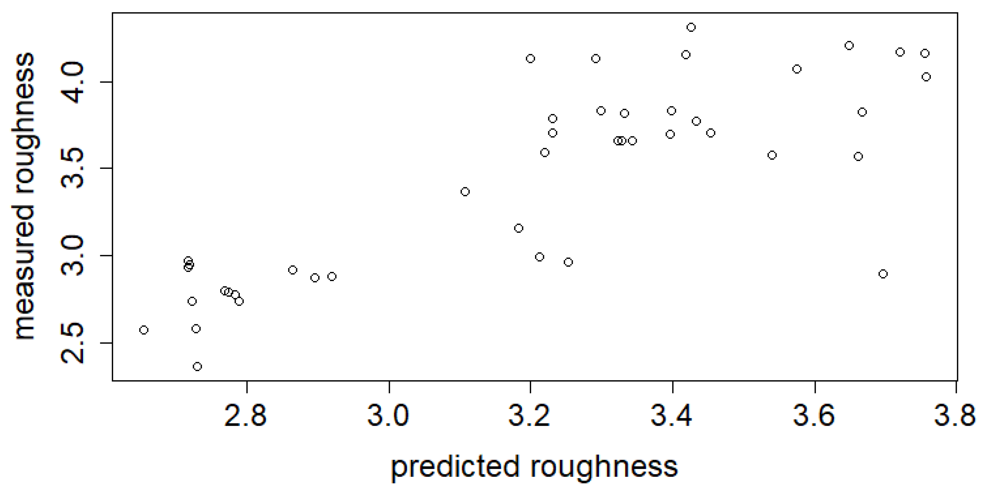
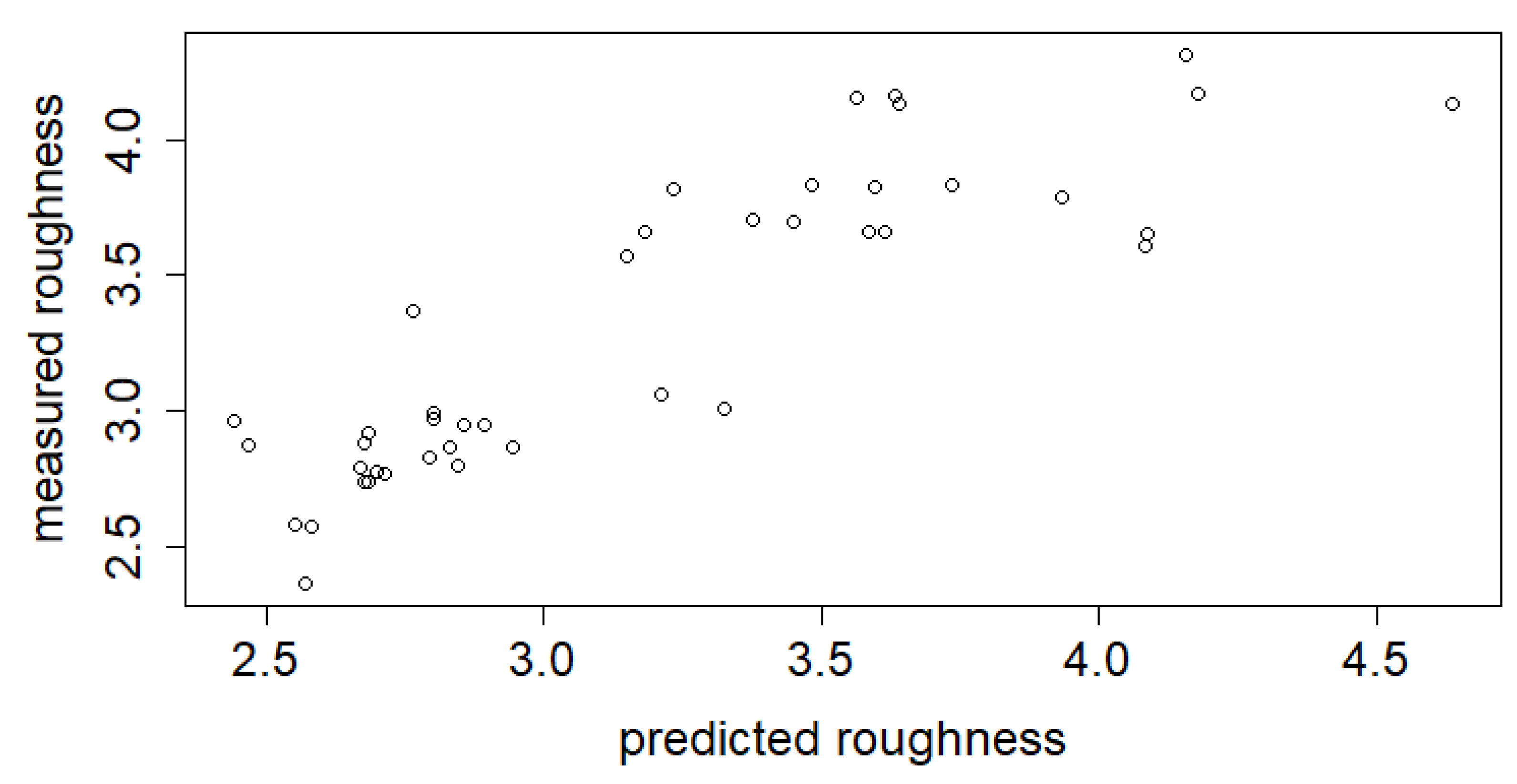
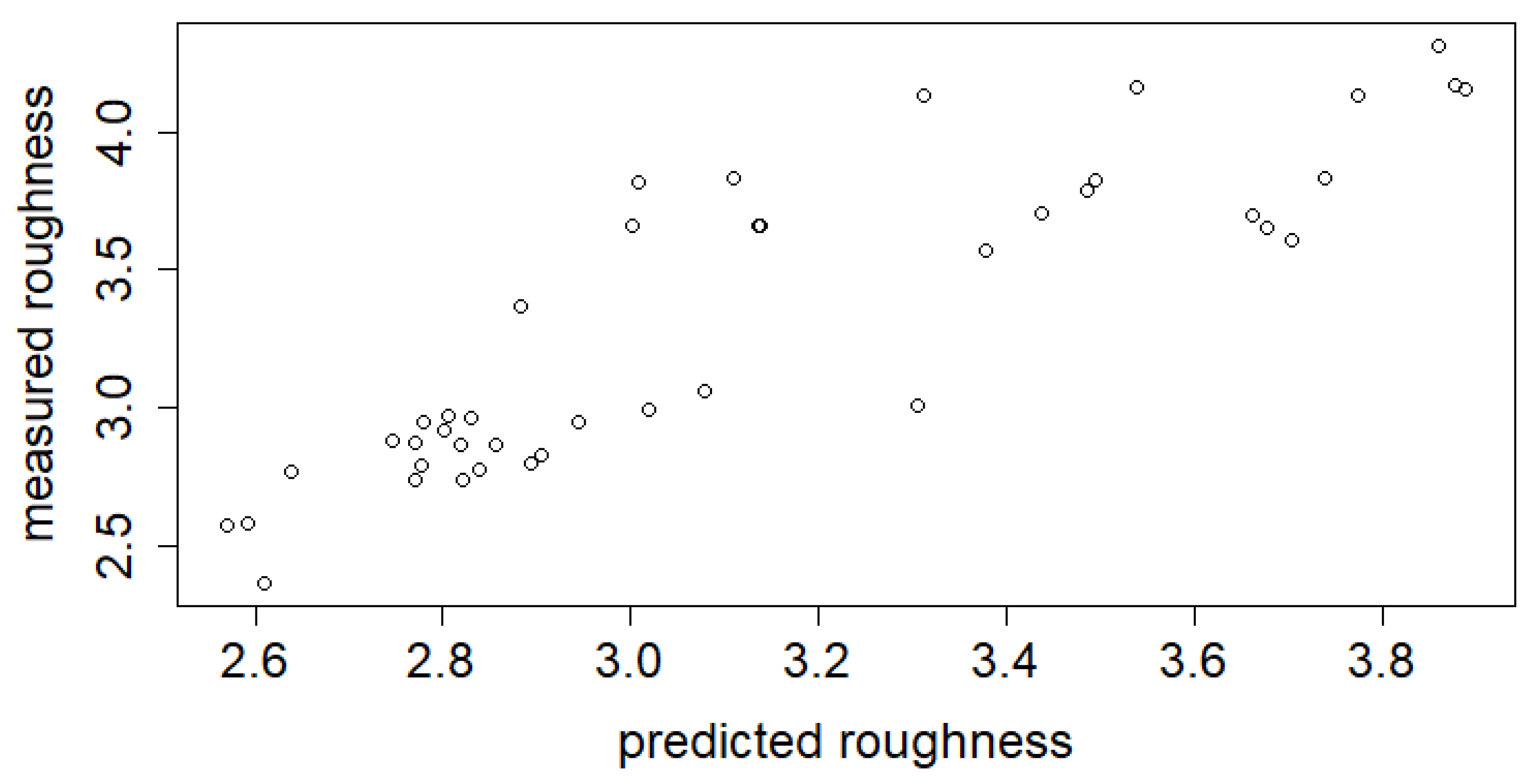
R	0.81	0.87	0.87

. The overall correlation between the target and estimated values of the test set was 0.87 for Model_HYBRID, 0.87 for Model_RAP, and 0.81 for Model_HOT, respectively. Scatter plots for predicted and actual values can be seen in Figure 1, Figure 2 and Figure 3. The observations in Model_HOT are a bit more scattered than in Model_RAP and Model_HYBRID. Figure 1 shows that Model_HOT cannot produce a predicted roughness greater than 3.8. In contrast, Model_RAP and Model_HYBRID perform better, as can be seen in Figure 2 and Figure 3. According to the root mean squared errors (RMSEs), the variables of the RAP line can actually explain the surface roughness better when compared to Model_HOT; the difference between RMSEs is 0.1. The difference between Model_RAP and Model_HYBRID is marginal. The later analysis will reveal some reasons for the weaker performance of Model_HOT.

6. XAI Empowered Decision Support

A machine learning model produces a predicted value for the quality of interest, but in evidence-based decision support, there is a need for explained results as well. Visualization of the models improves the understandability of the results. In addition, the trustworthiness can be increased when the user can verify the relations of the model with the domain knowledge.

6.1. Variable Importance

In GBM, the relative importance of the input variables is determined by their occurrence on the splits during the tree building process and how much each variable then improves the MSE (mean squared error) of the whole prediction model. The importance of the variables of each model for roughness prediction are presented in Figure 4, Figure 5 and Figure 6. In Model_HOT (Figure 4), the variables that come up are specifically related to tandem rolling (TA) and roughing mill (RM), and the most important are the reduction of the strip at first tandem pass (HOT REDUCTION TA), the specific force of the second (middle) tandem pass (HOT SPECIFIC FORCE TA2), and the rolling force in the middle part of the strip during the first tandem pass (HOT MID ROLL FORCE TA). From the chemical composition of the steel strip, only niobium (NB) has a significant influence. The rolling variables relate the pressure of the roll on the surface and NB contributes to the strength of the strip, and thus they may have a role in roughness forming, but indirectly, from the effect of mechanical properties. The most important variables in Model_RAP (Figure 5) are all related to the process speed, especially speeds related to pickling and shot blasting, and also slightly to annealing. This is natural, because the pickling speed tells us directly how long the acid attacks the surface and increases the roughness. The annealing speed in turn affects the mechanical properties and the capability of the products surface to resist the effects of the shot blasting. Furthermore, in Model_HYBRID (Figure 6), the RAP process and pickling speeds have a strong influence on roughness. There are also two hot rolling parameters in the top four of the most important parameters. These parameters are important in Model_HOT as well: the reduction of the strip at first tandem pass (HOT REDUCTION TA)) and the diameter of the roll at the fifth roughing mill pass (HOT ROLL DIAM RM5).

The hot rolling parameters relate strongly to mechanical properties. They may have an effect on surface roughness, but more likely, they are selected because of the strength of the steel. Roll diameter is an exception; it can relate to the area of surface that is in contact or the early phase with new rolls. Either one can be adjusted during the process, but production planning can use the information and schedule the products with the highest quality requirements to a campaign with lower risk. The answer to our first hypothesis is that we cannot improve the surface quality during the process by adjusting only the hot rolling parameters, and in their turn, the RAP variables can explain most of the problem. Thus, only Model_RAP is suitable for assisting the real-time adjustments by RAP-line operators. By combining the parameters from both hot rolling and RAP processes, we can create a hybrid model that gives a wider perspective on the processes. This model is useful for product and production planning and process engineers that want to learn the complete set of relationships. In following analyses, we present the results with Model_HYBRID only.

6.2. Model Interpretability

In manufacturing, the outcome is not only dependent on the process parameters independently, but also the interactions of the variables have an impact. In GBM, the interactions of the variables can be included in the model, and in this application, the interaction depth (the highest level of interactions between variables allowed during training the model) was three. Some of the variables may have quite a strong impact on interactions, but most of them do not interact actively with the other variables. In practice, the impact of the most important individual variables usually outperforms that of interactions. Figure 7 shows how strongly the variables of Model_HYBRID interact with each other based on the test set data. The interaction strength value corresponds to the proportion of explained variance of $f\left(x\right)$ for each feature. The value is located between 0 when there is no interaction and 1 when all variation depends on a given feature’s interactions. Clearly, the variable with the most interactions is the RAP speed. Additionally, the diameter of the roll in the fifth roughing mill pass, the reduction of the strip at first tandem pass, and the average pickling speed are on top of the interaction list. However, overall, the interaction strengths are quite weak. For each feature, it is possible to find the strongest interaction partners as well. In Figure 8, the interactions between the most important feature—the RAP speed—and other features are shown. The strongest pair is the RAP speed and the diameter of the roll at the fifth roughing mill pass (HOT ROLL DIAM RM5). However, overall, the values for the majority of the interaction pairs are quite low.

With Partial Dependence Plots (PDP), the effect of each variable on the response variable can be visualized together with the distribution of data points. From PDP in Figure 9 and Figure 10, it is quite clear that the faster the steel strip goes, the lower the risk of surface roughness is in RAP-line. The decrease in roughness appears especially after 60 km/h. Figure 11 shows the relation between the diameter of the roll at the fifth roughing mill pass (HOT ROLL DIAM RM5) and the predicted response variable. The larger the diameter of the roll is (>96,000), the larger the risk of roughness is. Figure 12 presents the reduction of the strip at the first tandem pass (HOT REDUCTION TA). Clearly, with a reduction larger than 1.25, the risk of roughness is lower. To obtain a larger reduction, a larger rolling force is needed. The rolling force is proportional to the width of the strip and it relates to the pressure on the surface of the strip. Thus, it affects the quality of the surface. Some specific products, which are softer and more delicate as a result of their other mechanical properties, need to be rolled in a more sensitive way, and thus the rolling force and resulting reductions during individual passes are smaller as well.

Figure 13 shows the PDP of roughness and the interaction of the diameter of the roll at the fifth roughing mill pass and the speed of the RAP process, which is the pair of variables with the strongest interaction, as shown in Figure 8. As can be seen, roughness is at its lowest with a diameter of the roll under 960,000 and with a speed over 90. Roughness is at its highest with low speeds (<60) and especially when combined with a high diameter of the roll (>980,000). This tool is especially useful if the user needs to compromise between two parameters when trying to find the best manufacturing settings.

The accumulated local effects (ALE) plots can be used in addition with PDP to visualize the effect of selected variables on the dependent variable, as well. In Figure 14, ALE shows the main effect of the average pickling speed on the prediction of the surface roughness and the distribution of data points, and in Figure 15, the main effect of the diameter of the roll at the fifth roughing mill is shown. As can be seen, the prediction of roughness crosses the horizontal zero level when the average pickling speed is about 78 km/h; in other words, the prediction of roughness is lower with a pickling speed greater than 78 km/h, whereas the prediction of roughness is larger when the diameter is larger than 960,000. ALE analysis reveals that the surface roughness of the steel strip is a bigger problem with lower speed values related to the RAP process, and clear speed limits for lower roughness risk can be defined based on ALE analysis.

6.3. Visualizations for an Individual Product

When a high rejection risk is predicted for a single product, the user needs information that may help to prevent the actual failure. SHAP visualizations enable the inspection of the reasons behind the estimation for each observation individually. The selection of the reference group has to be done carefully, because the visualization should reveal the difference between the prediction of the current observation and the average prediction result of the other similar products. The comparison should not be conducted for the whole production, because the revealed differences should be potentially harmful process settings within a product group instead of the natural differences between the product types. An example with a bad roughness prediction demonstrates the usability of the method in Figure 16. As can be seen, the prediction for roughness is 3.74 for the bad version, while the average prediction is 2.96 for this steel type in general. The phi value describes the strength of each feature value contribution in the prediction. For this product, the strongest candidates for a poor prediction are low RAP and pickling speeds. In addition, the slightly high diameter of the roll at the fifth roughing mill pass indicates the risk of roughness. The variable values in SHAP visualization do not reveal in which direction the value should be adjusted in order to improve the product quality. Thus, it would be advisable to complement the SHAP visualization by returning to PDP visualizations. For this product, the RAP speed of 50.75 and the average pickling speed of 54.59 are found on the left side in Figure 9 and Figure 10, which relate to the worst surface quality, and an increase of 20 units in the speed could improve the quality dramatically. Furthermore, the diameter of the roll increases the expected roughness (Figure 11). Based on Figure 12, the reduction of the steel strip at the first tandem pass is 1.26, which relates to the better surface quality, but the effect is not strong enough to overcome the negative factors.

Instead of complementing the SHAP results interpretation with the PDP plots, the user can also utilize the empirical distributions of the process data. It is interesting to see where the observed product is found when compared to successful products in its product group. With parallel coordinates, the user can immediately pinpoint the variables that most probably contribute to the poor prediction, but opposed to the SHAP visualization, the direction of divergence of the variable value can also be seen. In Figure 17, the parallel coordinates plot for the product from the previous example is presented. Each line represents one observation; the left column is the predicted roughness, and the following columns are the variables selected for observation based on their importance in the prediction model. A high impact in the model correlates with impact in the defect prediction, and thus the high-impact variables are the best candidates to cause the defect, if the distance to the good variables is visible. For actual use, the visualization can be implemented to allow the user to select the visualized variables alternatively. An observation with an increased risk of roughness has been indicated with a black line, and the good products in the same product group are presented with the green lines. As can be seen, the high-risk observation diverges from the good products for several variables; this product has low speeds, a slightly high diameter of the roll, and high bending in the middle of the strip during tandem rolling.

The parallel coordinate information can be derived to create another easy-to-understand visualization type. Figure 18 presents the scaled distances of each variable between the bad product and the good products. This information can be utilized as a recommendation for actions in automated decision support systems. Figure 19 shows the distance information as a simple visualization. This visualization type is especially useful in situations that require immediate decisions. The view shows only the potential variables that could be adjusted in order to decrease the risk of roughness. Naturally, it is important to use a model with the variables that the operators can actually adjust during the production. Figure 20 shows the same visualization type based on the Model_RAP, which can be offered to operators in the RAP-line.

7. Discussion and Conclusions

The need for decision support tools that are able to produce alarms for product failure risks and recommendations for preventive actions is critical for today’s manufacturing industries. This article presents a solution that utilizes machine learning prediction models and XAI methods for automated data quality monitoring and root cause analysis. Although a steel making process was selected to demonstrate the method, the concept is applicable in any manufacturing process where a product’s quality property is affected by the process variables.

7.1. Practical Aspects to Decision Support Development in Industry

The decision support tool development contained several steps from data collection and model development to model analytics and visualization based on the user’s needs. The lessons learned are generalizable to a wider audience regardless of the field. The following aspects were recognized while employing and using manufacturing data for quality improvement and decision support in industry.

Data collection. If possible, the data collection should be designed for decision support purposes. Data should contain a comprehensive set of products and production conditions with relevant parameters. In the presented application, the available data contained only a fraction of the actual repertory. In order to improve the generalizability of the model, an investment into collecting a larger data set could be made. This is advisable, especially if the model proves to be useful in product and production planning.

Surrogate model. It is possible to use model predictions as surrogates for actual measurement device. At Outokumpu, the absence of a surface roughness measurement device on site prevented the prediction of this quality property earlier. This article demonstrates that the surface roughness of the steel strip can be predicted with good accuracy, and the risk of a failure can be presented to the user already during the product planning phase, which enables the user to adjust the process parameters and minimize the risk of roughness. Even though the measurement campaign has ended, it is still possible to adjust the process based on the predicted quality and to improve the surface quality. Naturally, the model’s performance in real-time use cannot now be verified.

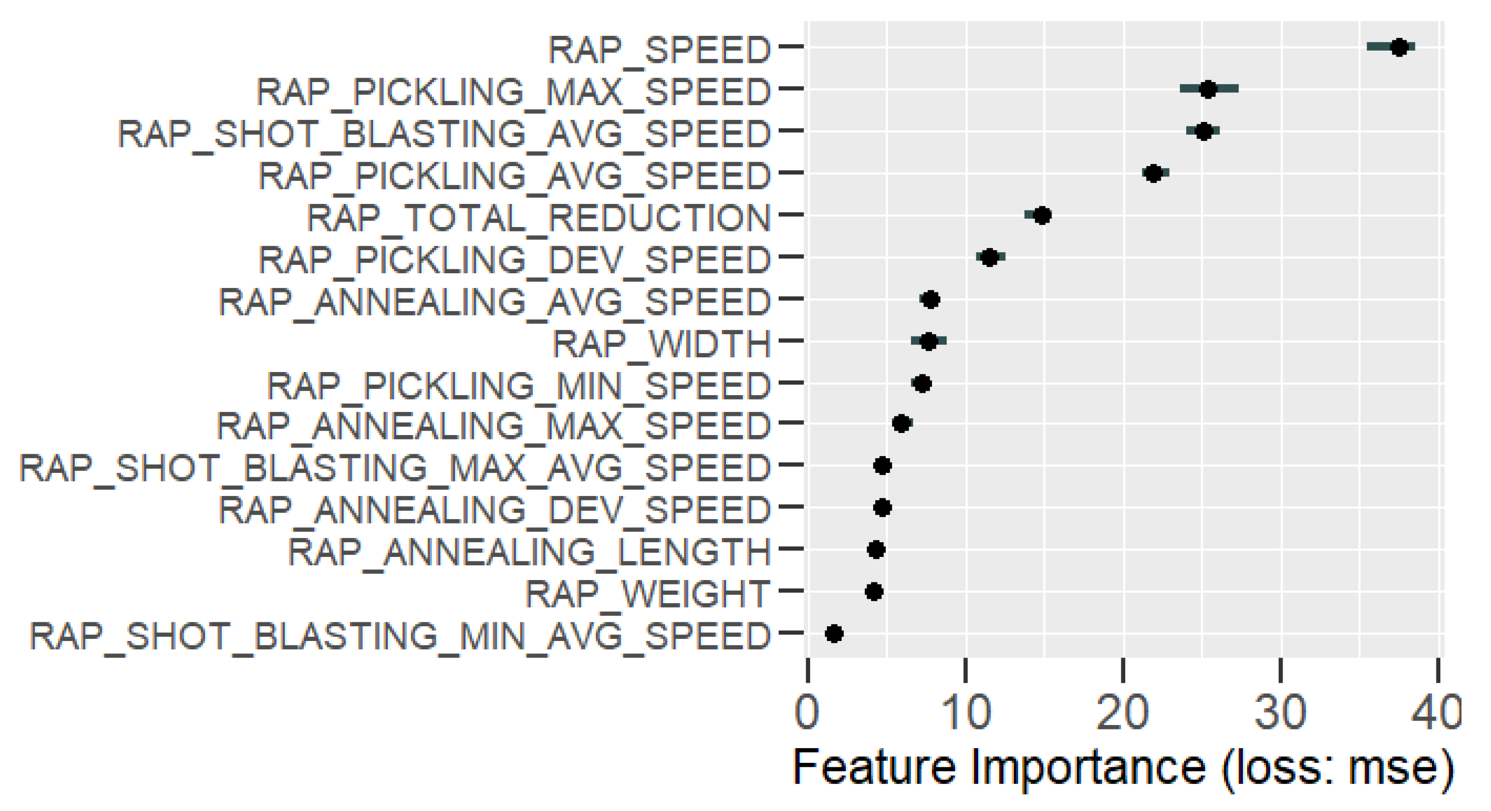
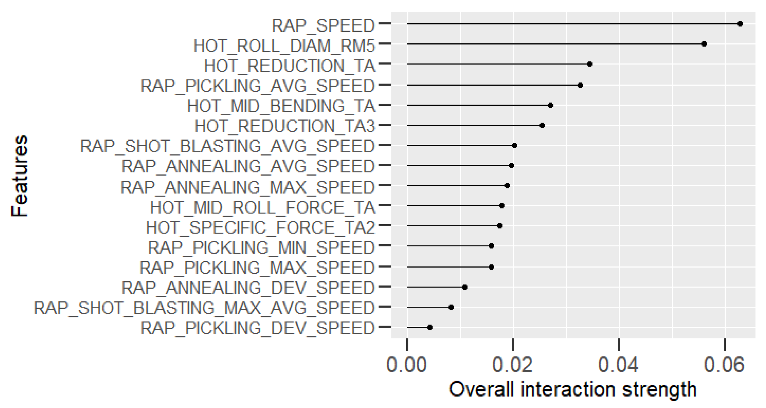
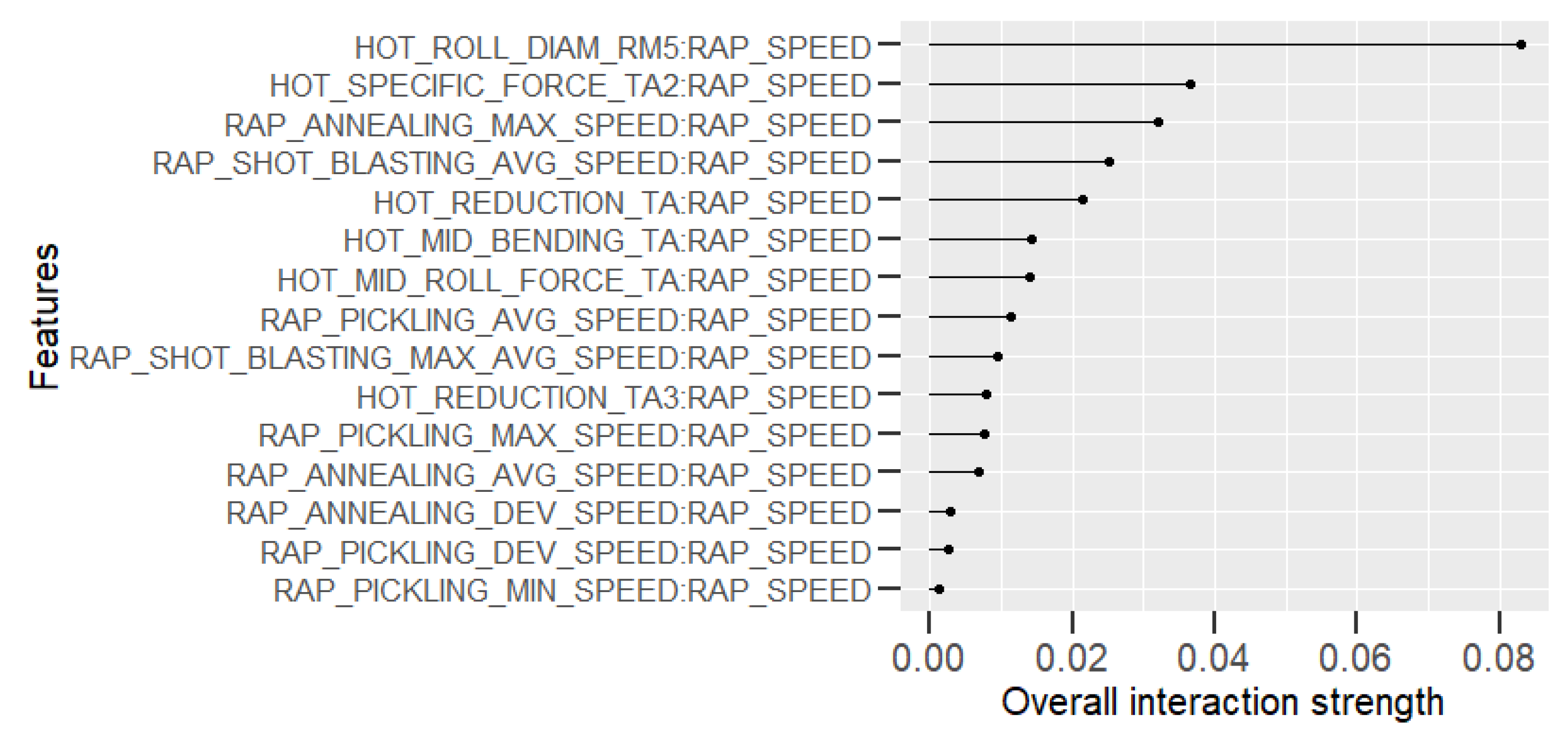
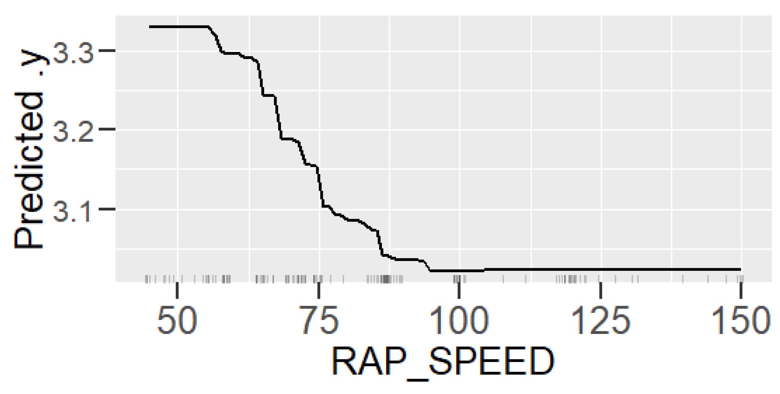
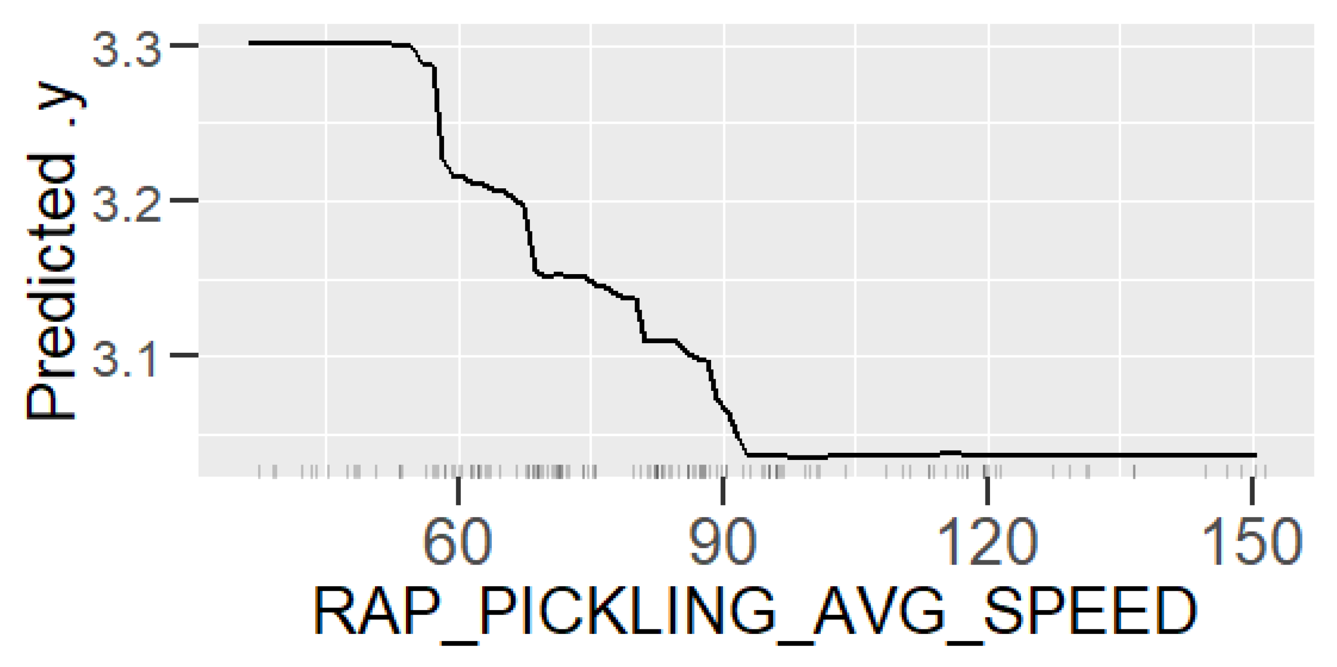
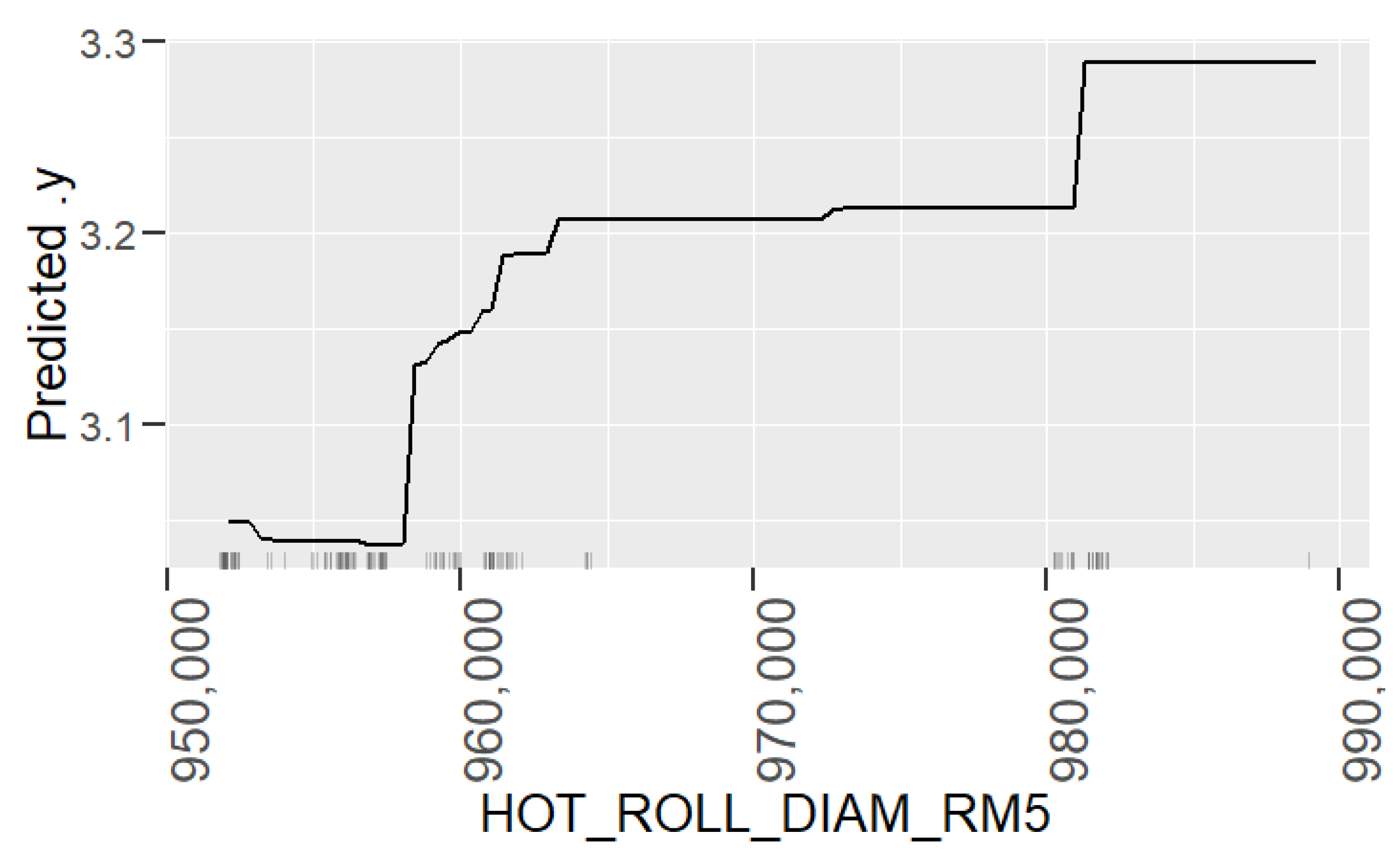
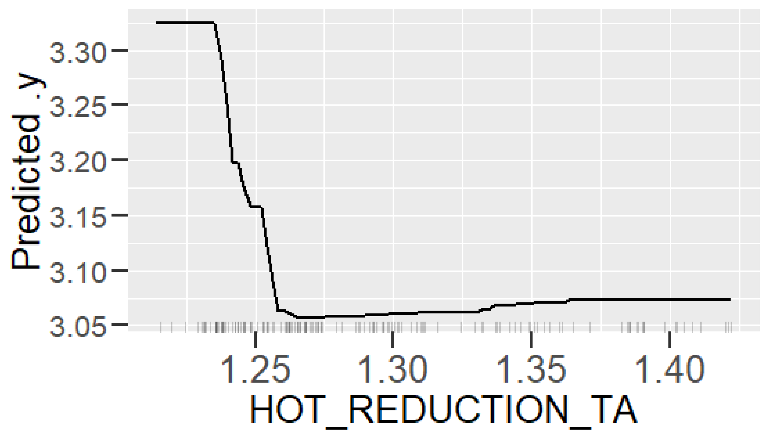
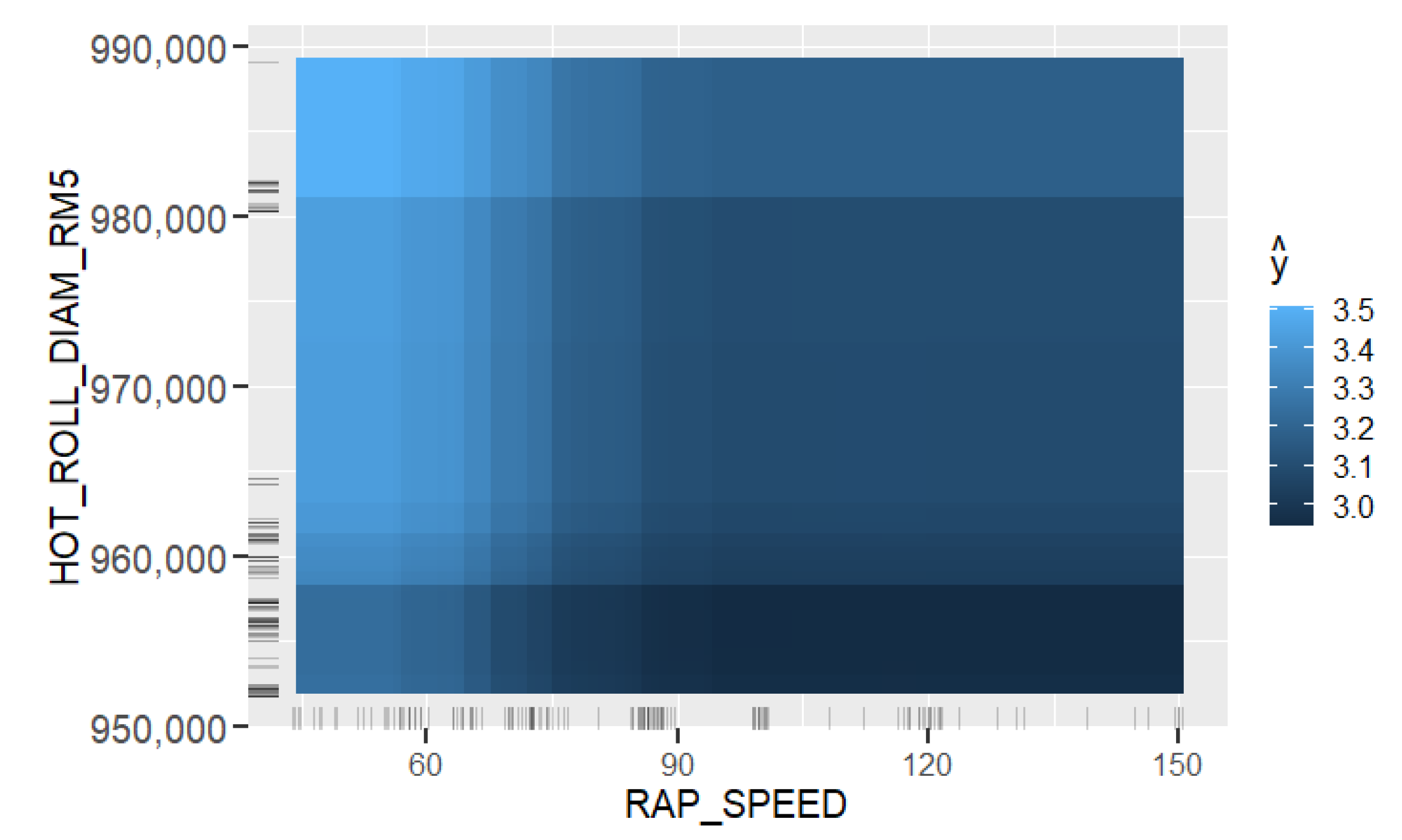
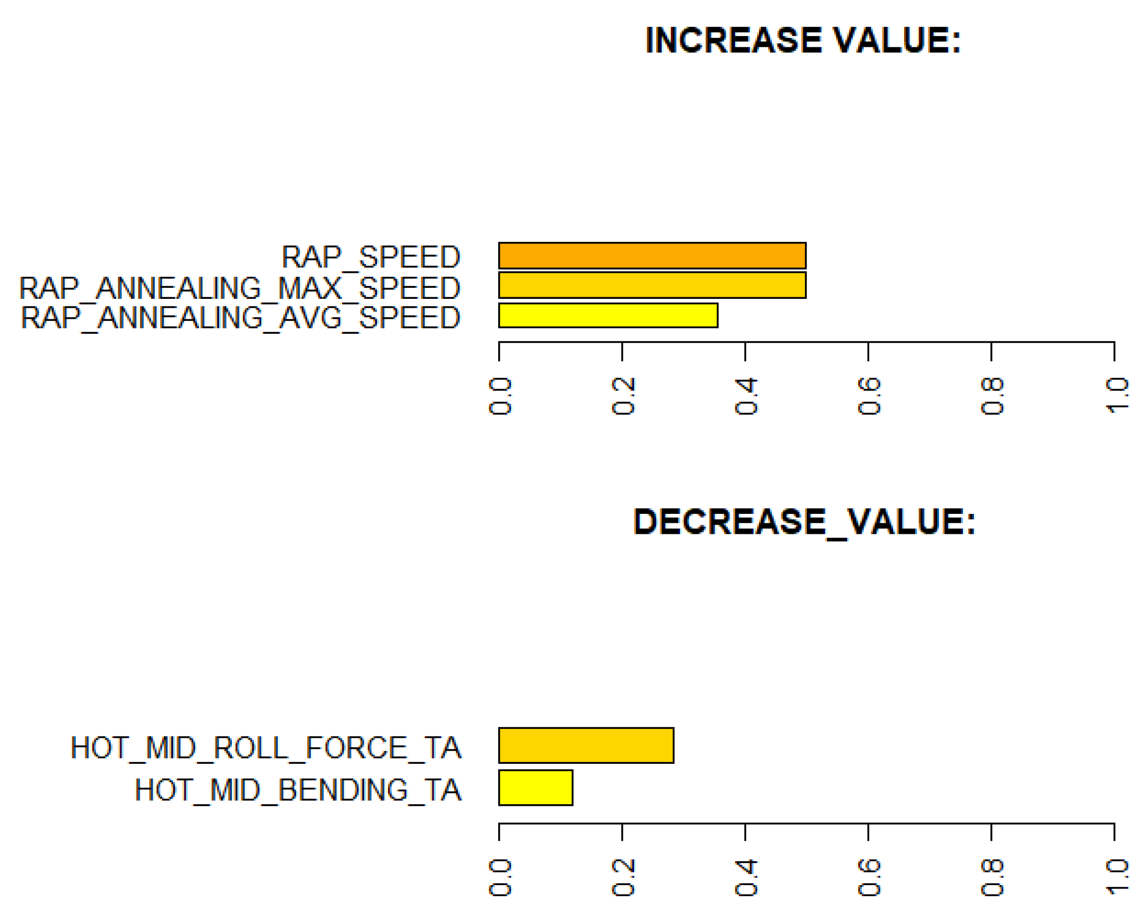
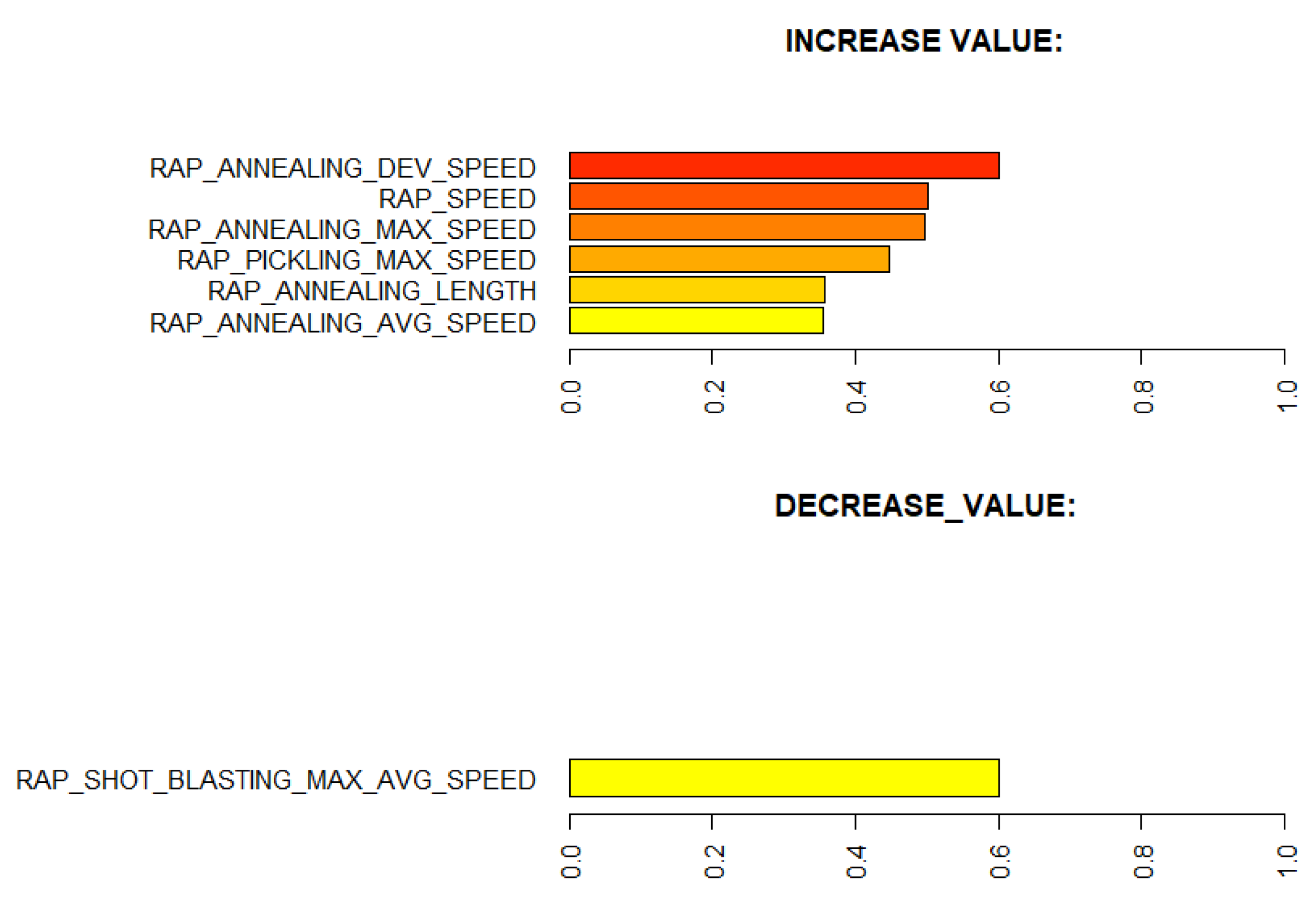
Learning the process. With prediction models, it is possible to obtain an insight into production and better understand the relationships between process parameters and the predicted property. In this case, the analysis of the roughness prediction models uncovered the parameters of the RAP-line that have the highest impact on the surface roughness. Additionally, the hypothesis for the high importance of the hot rolling process parameters on roughness formation was disproved. The hybrid model and RAP model outperformed the HOT model. Actually, the parameters in hot rolling reflected especially the mechanical properties of the product and inherently the probable surface quality. The difference in roughness appeared mainly because of the varying RAP line parameters when comparing products with similar mechanical properties. By studying the visualizations of the model’s performance, the user may learn more about the process and how the parameter settings affect the quality and how they relate to each other.

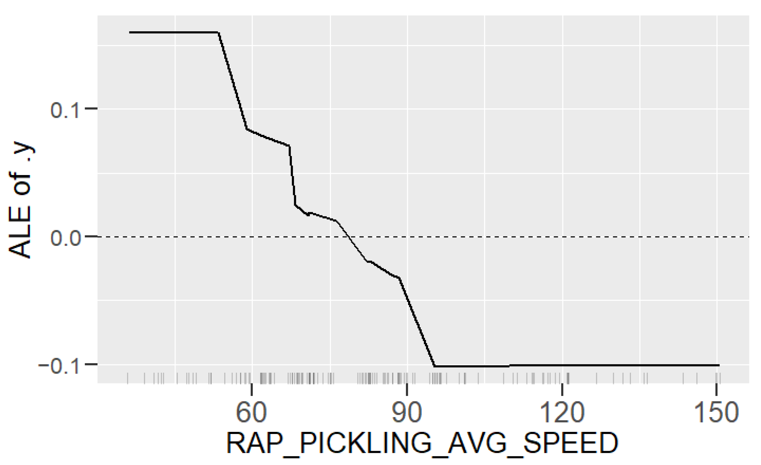
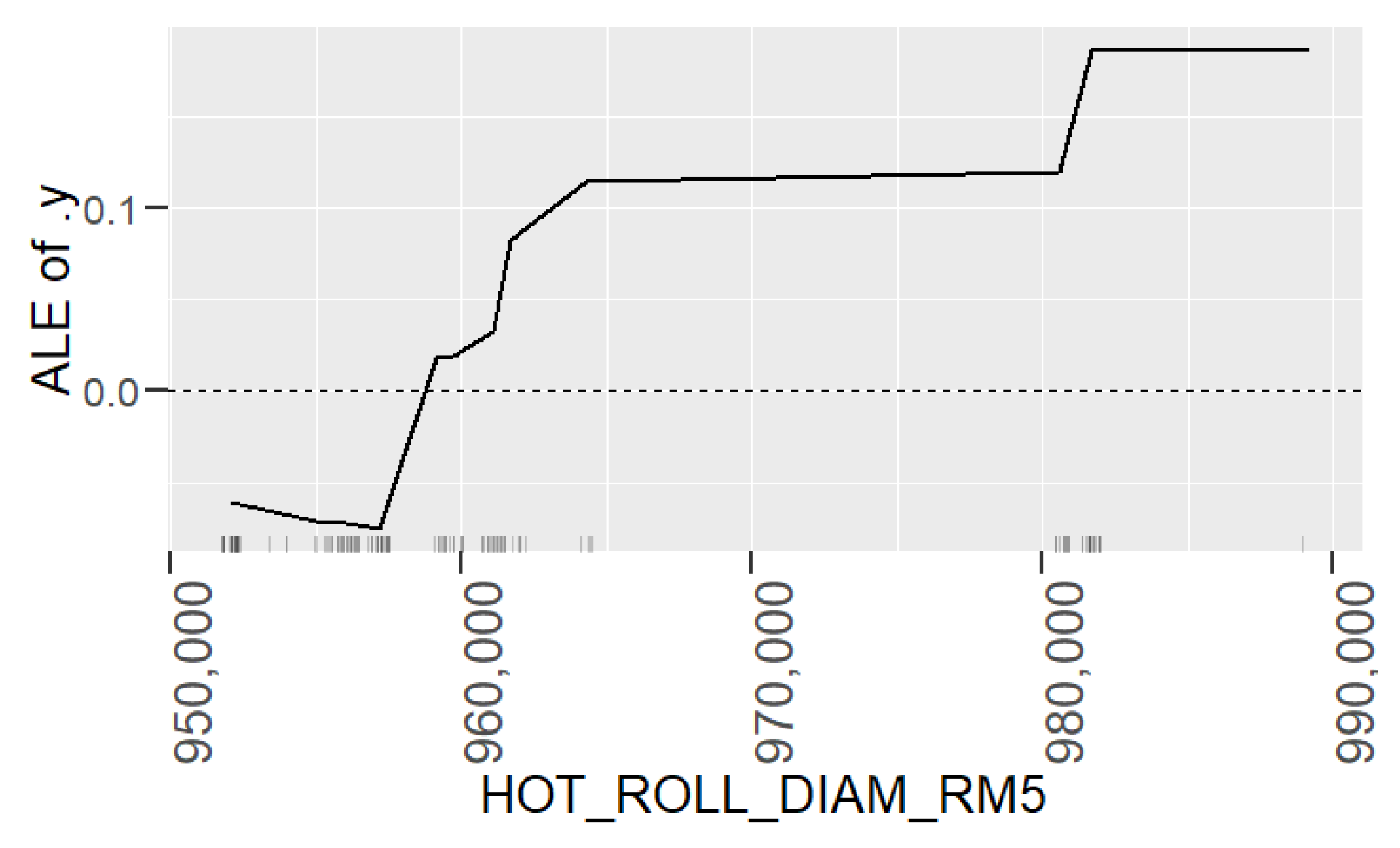
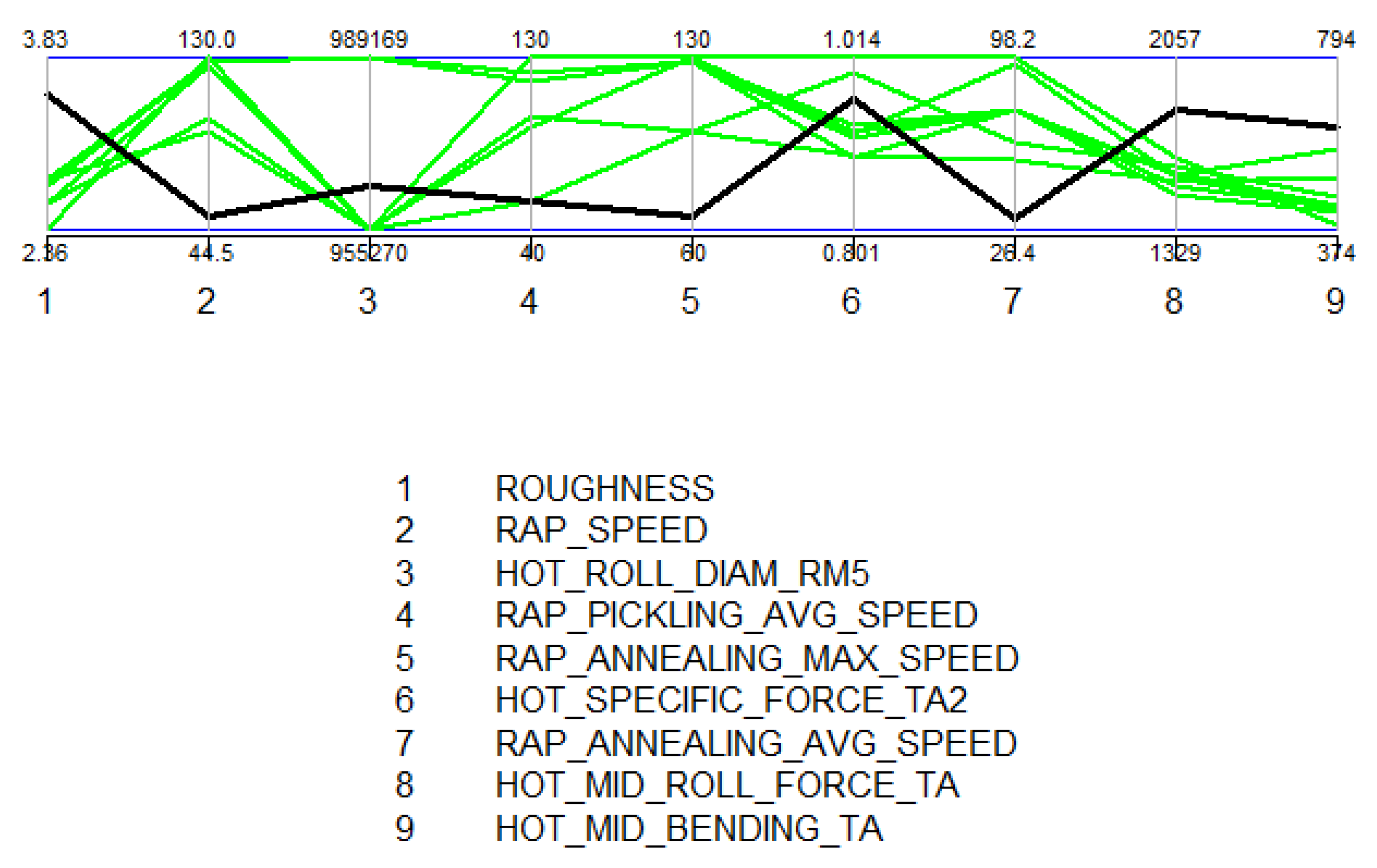
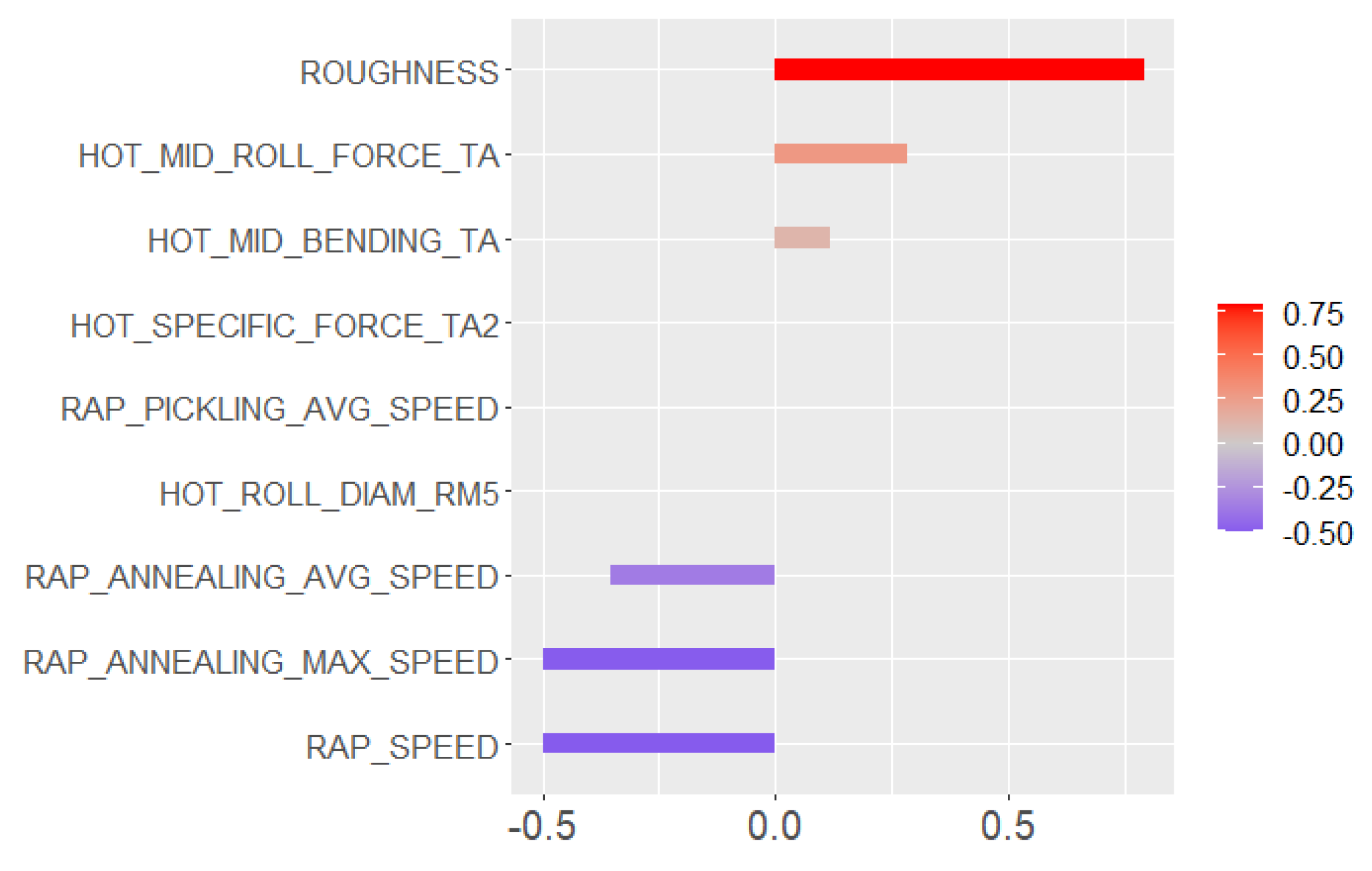
Creating new knowledge. It is important to understand the reasoning behind the predictions. This way, the user can verify the applicability of the results and evaluate the performance for individual observations. The interpretability of the models was improved with XAI methods (PDP, ALE, SHAP, parallel coordinates and its modifications) that highlight the significance of the process parameters in roughness formation individually for each observed product. The average performance of the model can be quite different for individual products as the chemical composition and mechanical properties determine how each product type responds to the process settings during the manufacturing. Thus, it is important to find out the rootncauses behind a high predicted risk of failure.

Role of domain knowledge. It is important to emphasize that the methods presented in this article cannot replace the domain knowledge; the final decision is still made by the human experts, and the strength of the proposed tool is in its capability to process large amounts of data and highlight the information in it. It is not always possible to adjust the harmful parameter to a more favorable direction, because of the product property requirements or the overall optimization of the process; the settings that guarantee high surface quality may not guarantee other quality properties that the product has. In addition, some of the parameters describe the status of the machines; the wearing of the rolls, for example. Then, the re-scheduling of the production is the only way to optimize the parameters and to find the best process conditions for the most demanding products.

Role of the user. In order to gain a large group of potential users, the tool should contain different types visualizations for different user’s needs. In a steel plant, the users of the decision support tools may have different needs based on their duties. In product design and process planning, the process engineers may want to test different settings and thus learn about the whole process, while the process operators have a different objective with a very short reaction time. In this case, the detailed visualizations of variable impacts and dependencies can be observed with time, while the simple presentation of possible actions for quality improvement works, when selecting the correct process settings for a product rapidly.

Uncertainty of models. When in actual use, if data are not complete, the user should be informed about the uncertainty of prediction when the system is extrapolating. The other possibility would be to restrict the usage of the tool to known products only. In the case of this study, the data were not collected for research purposes and were not very representative. The models could easily be improved by systematically collecting data from production.

7.2. Future Work

In this research, the practical usability was the main motivation when selecting the models and techniques. All developed tools can be integrated into an existing quality monitoring tool that has connections to process databases and the capability of running R scripts and producing the required predictions, visualizations, and decision support. This way, the potential users in the steel plant can obtain access to the tool with a web-based user interface.

After implementation, the tool can be tested by users in different roles. The need for a new measurement campaign was recognized and the data collection can be designed based on the test results. The test phase may reveal a need for systematic data collection from different product types or production periods. The model accuracy can be improved by increasing the amount of training data, and also the generalization capability of models can be verified better. In addition, the need for personnel training can be recognized with the analysis of the results. The motivation to use the tool is directly dependent on its usability and benefits.

References

1. Oakland, J.S. Statistical Process Control; Routledge: London, UK, 2007. [Google Scholar]
2. Zhang, Y.; Cheng, Y.; Wang, X.V.; Zhong, R.Y.; Zhang, Y.; Tao, F. Data-driven smart production line and its common factors. J. Adv. Manuf. Technol. 2019, 103, 1211–1223. [Google Scholar] [CrossRef]
3. Fayyad, U.M.; Piatetsky-Shapiro, G.; Smyth, P. From Data Mining to Knowledge Discovery: An Overview. In Advances in Knowledge Discovery and Data Mining; MIT Press: Cambridge, MA, USA, 1996; pp. 1–34. [Google Scholar] [CrossRef]
4. Phillips-Wren, G. Intelligent Decision Support Systems. In Multicriteria Decision Aid and Artificial Intelligence; John Wiley & Sons, Ltd.: Chichester, UK, 2013. [Google Scholar]
5. Braha, D. (Ed.) Data Mining for Design and Manufacturing: Methods and Applications; Kluwer Academic Publishers: Norwell, MA, USA, 2002. [Google Scholar]
6. Logunova, O.S.; Matsko, I.I.; Posohov, I.A.; Luk’ynov, S.I. Automatic system for intelligent support of continuous cast billet production control processes. Int. J. Adv. Manuf. Technol. 2014, 74, 1407–1418. [Google Scholar] [CrossRef]
7. Xu, L.; He, W.; Li, S. Internet of Things in Industries: A Survey. IEEE Trans. Ind. 2014, 10, 2233–2243. [Google Scholar] [CrossRef]
8. He, S.; Wang, G.A.; Li, L. Quality improvement using data mining in manufacturing processes. In Data Mining and Knowledge Discovery in Real Life Applications; Ponce, J., Karahoca, A., Eds.; I-Tech: London, UK, 2009; pp. 357–372. [Google Scholar]
9. Wang, K. Applying data mining to manifacturing: The nature and implications. J. Intell. Manuf. 2007, 18, 487–495. [Google Scholar] [CrossRef]
10. Tamminen, S.; Tiensuu, H.; Ferreira, E.; Helaakoski, H.; Kyllönen, V.; Jokisaari, J.; Puukko, E. From Measurements to Knowledge—Online Quality Monitoring and Smart Manufacturing. In Advances in Data Mining. Applications and Theoretical Aspects; Perner, P., Ed.; Springer International Publishing: Cham, Switzerland, 2018; pp. 17–28. [Google Scholar]
11. Bustillo, A.; Urbikain, G.; Perez, J.M.; Pereira, O.M.; Lopez de Lacalle, L.N. Smart optimization of a friction-drilling process based on boosting ensembles. J. Manuf. Syst. 2018, 48, 108–121. [Google Scholar] [CrossRef]
12. Nahavandi, S. Industry 5.0—A Human-Centric Solution. Sustainability 2019, 11, 4371. [Google Scholar] [CrossRef] [Green Version]
13. Goebel, R.; Chander, A.; Holzinger, K.; Lecue, F.; Akata, Z.; Stumpf, S.; Kieseberg, P.; Holzinger, A. Explainable AI: The New 42? In Machine Learning and Knowledge Extraction; Holzinger, A., Kieseberg, P., Tjoa, A.M., Weippl, E., Eds.; Springer International Publishing: Cham, Switzerland, 2018; pp. 295–303. [Google Scholar]
14. Hagras, H. Toward Human-Understandable, Explainable AI. Computer 2018, 51, 28–36. [Google Scholar] [CrossRef]
15. Friedman, J.H. Stochastic Gradient Boosting. Comput. Stat. Data Anal. 2002, 38, 367–378. [Google Scholar] [CrossRef]
16. Yin, S.; Kaynak, O. Big Data for Modern Industry: Challenges and Trends [Point of View]. Proc. IEEE 2015, 103, 143–146. [Google Scholar] [CrossRef]
17. Nguyen, T.L. A Framework for Five Big V’s of Big Data and Organizational Culture in Firms. In Proceedings of the 2018 IEEE International Conference on Big Data (Big Data), Seattle, WA, USA, 10–13 December 2018; pp. 5411–5413. [Google Scholar]
18. Garcia, S.; Luengo, J.; Herrera, F. Data Preprocessing in Data Mining; Springer: Cham, Switzerland, 2014. [Google Scholar]
19. Chang, Y.; Lin, S.; Liou, H.; Chang, C.; Wu, C.; Wang, Y. Improving the Surface Roughness of Pickled Steel Strip by Control of Rolling Temperature. J. Mater. Eng. Perform. 2013, 22, 322–329. [Google Scholar] [CrossRef]
20. Wei, D.B.; Jiang, Z.Y.; Huang, J.X.; Zhang, A.W.; Shi, X.; Jiao, S.H. Study on Surface Roughness and Friction during Hot Rolling of Stainless Steel 301. Advances in Materials Processing X. Trans Tech Publications. Adv. Mater. Res. 2012, 500, 403–409. [Google Scholar] [CrossRef] [Green Version]
21. FocalSpec. Available online: https://lmi3d.com/focalspec-line-confocal-sensors/ (accessed on 28 June 2021).
22. Linardatos, P.; Papastefanopoulos, V.; Kotsiantis, S. Explainable AI: A Review of Machine Learning Interpretability Methods. Entropy 2021, 23, 18. [Google Scholar] [CrossRef] [PubMed]
23. Friedman, J.H. Greedy function approximation: A gradient boosting machine. J. Ann. Stat. 2001, 29, 1189–1232. [Google Scholar] [CrossRef]
24. Apley, D.W. Visualizing the Effects of Predictor Variables in Black Box Supervised Learning Models. Stat. Methodol. 2016, 82, 1059–1086. [Google Scholar] [CrossRef]
25. Lundberg, S.M.; Lee, S.I. A Unified Approach to Interpreting Model Predictions. In Advances in Neural Information Processing Systems 30; Guyon, I., Luxburg, U.V., Bengio, S., Wallach, H., Fergus, R., Vishwanathan, S., Garnett, R., Eds.; Curran Associates, Inc.: Red Hook, NY, USA, 2017; pp. 4765–4774. [Google Scholar]
26. Inselberg, A. Visual Data Mining with Parallel Coordinates. Comput. Stat. 1998, 13, 47–63. [Google Scholar]
Figure 1. Scatter plot for predicted and actual values in test set for Model_HOT.
Applsci 11 10897 g001
Figure 2. Scatter plot for predicted and actual values in test set for Model_RAP.
Applsci 11 10897 g002
Figure 3. Scatter plot for predicted and actual values in test set for Model_HYBRID.
Applsci 11 10897 g003
Figure 4. Variable importance for Model_HOT.
Applsci 11 10897 g004
Figure 5. Variable importance for Model_RAP.
Applsci 11 10897 g005
Figure 6. Variable importance for Model_HYBRID.
Applsci 11 10897 g006
Figure 7. The strength of the interactions of the variables.
Applsci 11 10897 g007
Figure 8. Interaction between the most important variable and other variables.
Applsci 11 10897 g008
Figure 9. PDP of the speed of the RAP process.
Applsci 11 10897 g009
Figure 10. PDP of the average pickling speed.
Applsci 11 10897 g010
Figure 11. PDP of the diameter of the roll at the fifth roughing mill pass.
Applsci 11 10897 g011
Figure 12. PDP of the reduction of the steel strip at the first tandem pass.
Applsci 11 10897 g012
Figure 13. PDP of the roughness and the interaction of the diameter of the roll at the fifth roughing mill pass and the speed of the RAP process.
Applsci 11 10897 g013
Figure 14. ALE of the average pickling speed to the predicted roughness of GBM (black solid line) on the Y-axis and the distributions of data points (black bars) on the X-axis.
Applsci 11 10897 g014
Figure 15. ALE of the diameter of the roll at the fifth roughing mill pass to the predicted roughness of GBM (black solid line) on the Y-axis and the distributions of data points (black bars) on the X-axis.
Applsci 11 10897 g015
Figure 16. SHAP values for a bad product with a prediction of 3.74 for roughness, while the average prediction is 2.96 inside the group of the same steel type.
Applsci 11 10897 g016
Figure 17. Parallel coordinates for a product with an increased risk of roughness (solid black) compared to the set of good products (green).
Applsci 11 10897 g017
Figure 18. Scaled deviated variable distances that are potential root causes for a bad predicted quality.
Applsci 11 10897 g018
Figure 19. Recommended actions for an operator when a product has a bad predicted quality with Model _HYBRID.
Applsci 11 10897 g019
Figure 20. Recommended actions for an operator when a product has a bad predicted quality with Model _RAP.
Applsci 11 10897 g020