A Stable and High-Precision Downward Continuation Method of Magnetic Data

Abstract

Downward continuation is an effective technique that can be used to transform the magnetic data measured on one surface to the data that would be measured on another arbitrary lower surface. However, it suffers from amplitude attenuation and is susceptible to noise, especially when the continuation distance is large. To solve these problems, we present a stable and high-precision downward continuation method combining the ideas of equivalent source technique, Tikhonov regularization, radial logarithmic power spectrum analysis, and constrained strategy. To implement this method, the observed data is used to construct the equivalent source in the study area, and the small amount of measured magnetic data at the lower surface (relative to the original observation surface) is employed to constrain the calculation procedure simultaneously. Then the magnetic data at the target surface can be obtained by using a forward calculation procedure instead of the risky downward continuation procedure. The proposed method is tested on both synthetic model data and real magnetic data collected in the South China sea. Various obtained results demonstrate that the method reported in this study has higher accuracy and better noise resistance than the traditional downward continuation methods.

1. Introduction

Downward continuation of magnetic data can be used to obtain the magnetic data measured on one surface to the data that would be measured on another arbitrary lower surface, with which the high frequency information induced by the causative sources can be enhanced. Over the years, it has been widely used in many practical applications [1,2,3,4,5,6,7,8,9,10,11,12,13,14,15,16]. However, it suffers various disadvantages such as the non-convergence of the continuation operator, amplitude attenuation, and susceptibility to noise. Therefore, the downward continuation method has been the research focus over the past decades.

Generally, the theories for improving downward continuation can be summarized into three categories. The first category is reforming the downward continuation operator, such as using the Taylor series method to solve the operator non-convergence problem and applying the horizontal derivative to substitute the vertical derivative in the operator to stable the process [1,2,3,4]. The second category is replacing the downward continuation operators with other stable operators, such as adopting a three-order Adams–Bashforth formula method for downward continuation [5]. Using iterative upward continuation replaces the downward continuation process in the wavenumber domain [6,7,8] and combines the measured data of the lower interface with the Taylor series iterative method to derive the constrained downward continuation method [9]. The third is employing the equivalent source method to perform downward continuation, which is the main idea of this paper, and it is different from the above two categories. It simulates the forward process of the magnetic source rather than reforming or replacing the continuation operator and has been widely used in potential field data processing, such as magnetic and gravity anomaly transformation, potential filed data interpolation, and noise reduction of the observation data [10,11,12,13]. Because of its noise insensitivity and high continuation accuracy, this method also can be used in field continuation processing. For example, scholars have adopted a magnetic single-layer or dipole equivalent source to conduct continuation of aerial survey data, surface random point magnetic anomaly potential field data, and three component magnetic field data [14,15,16]. To further improve the accuracy of results, the wave number response of the regularized equivalent source has been studied, and then the iterative compensation algorithm and the optimization strategy of equivalent field source have been proposed [17,18,19]. Although above improved methods could stabilize the process and improve the precision indeed, most of these methods still have disadvantages such as susceptibility to noise and amplitude attenuation, especially when the continuation distance is large.

In this paper, we focus on reducing the impact of noise and improving the computational accuracy during the long-distance continuation. The measured magnetic data of the lower surface is used innovatively to constrain the construction of the equivalent source. The unbiased predictive risk estimator method (UPRE) is adopted to estimate the regularization parameters for achieving a stable result. The theoretical formulas of the presented method are provided. The feasibility of this method is investigated on synthetic and real data.

2. Methodology of the Proposed Method

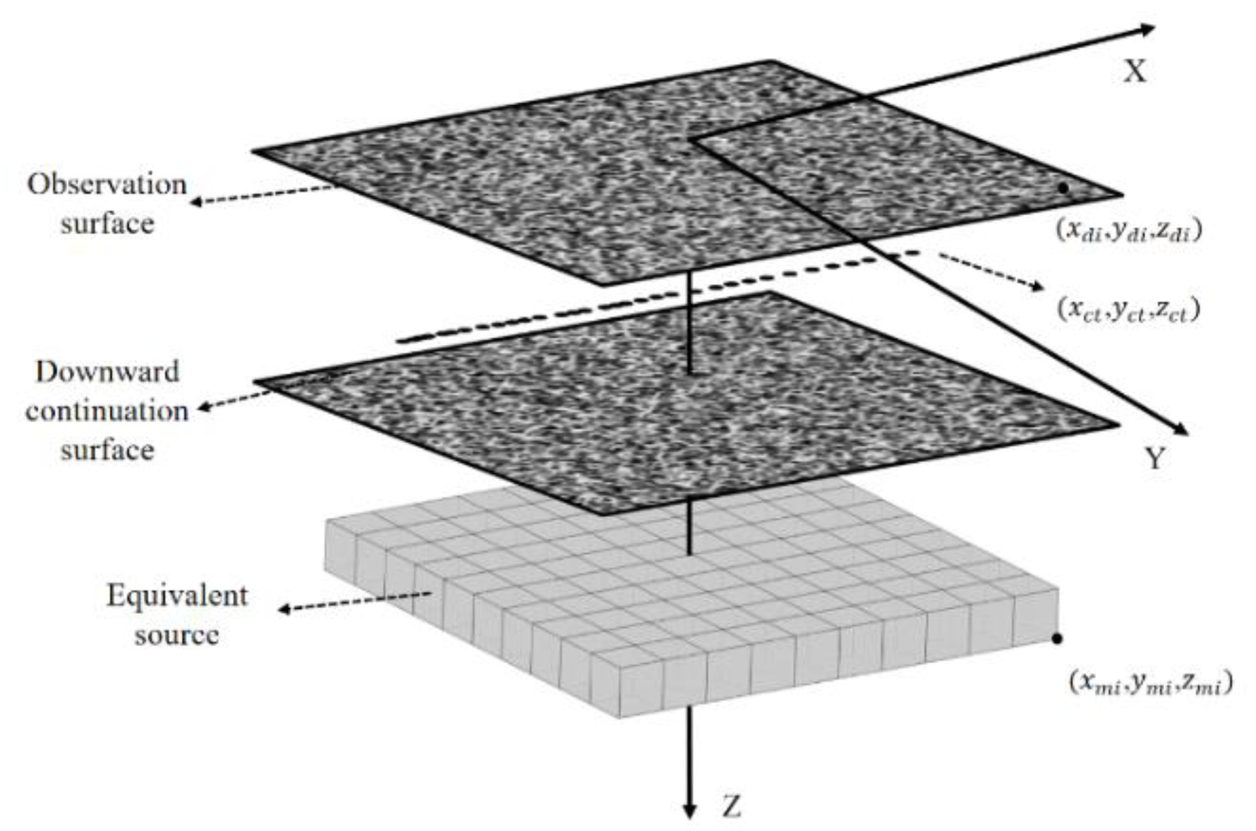
The proposed method is based on the equivalent source method; it is different from the conventional downward continuation technique, and there is no need to modify the continuation operator to amplify the signal, thus avoiding the influence of noise. It focuses on inverting a set of equivalent sources corresponding to the observed data, and then the magnetic data of the target depth can be obtained by forward calculation.

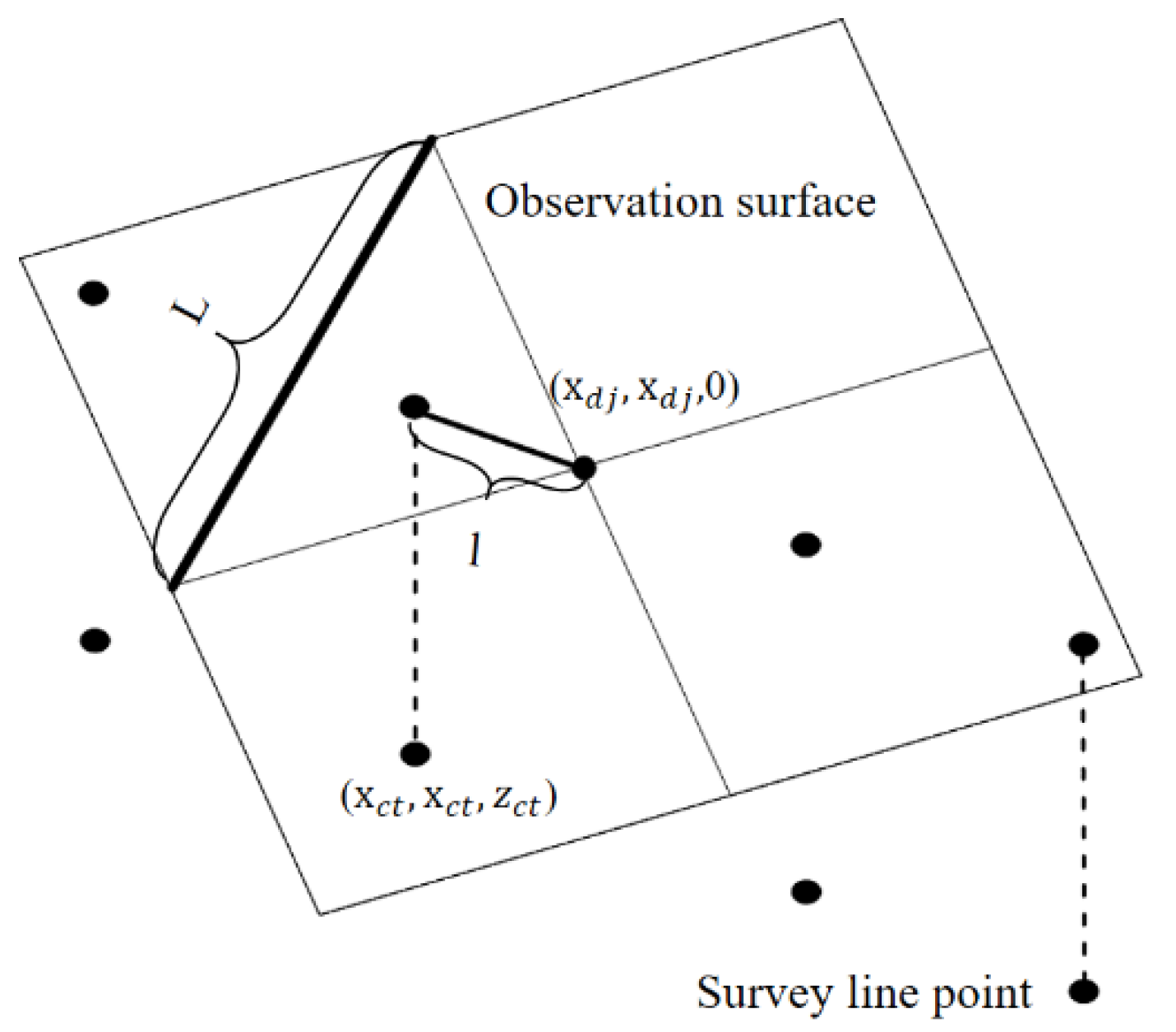
Figure 1 shows the space relationship of the observation surface, equivalent source cells, and measured data. However, the coordinates for measured data at the lower interface are hard to match with the observation network appropriately all the time. Therefore, its position needs to be interpolated to the observation network. We suppose that the coordinate of a constrained point is $(x_{ct},y_{ct},z_{ct})$ and the value is $d_{ct}$; its position at the grid is shown in Figure 2, and the nearest joint point is $(x_{dj},y_{dj},0)$.

Theoretically, the distance between the projection point of $(x_{ct},y_{ct},z_{ct})$ and its nearest joint point is $l=\sqrt{{(x_{ck}-x_{dj})}^2+{(y_{ck}-y_{dj})}^2}$. The longest distance in this grid is L, as Figure 2 shows. Following Equation (9), the position of the constraint in the grid can obtained by

$$\{\begin{array}{l}{x}_{ck}=x_{dj}\\ y_{ck}=y_{dj}\\ d_{ck}=d_{ck}\ast \cos (l\pi /2L)\end{array}$$

(1)

Then, we focus on the construction of the equivalent source. For establishing the relationship between the measured magnetic data and the equivalent source, the source layer is divided into a series of cells, with which the problem is transformed into a linear inversion problem whose matrix form is as follows:

$$d_{obs}=\mathbf{G}k$$

(2)

where $d_{obs}$ is the observed magnetic data vector, $k$ is the model susceptibility parameters to be solved, and the $\mathbf{G}$ is the model forward operator that has as elements $g_{ij}$, which describe the contribution of the susceptibility of the jth equivalent cell to the ith point at the observation surface gird. We assume the number of equivalent source cells and the observation data are M, N, respectively. The constraint data is $d_{ct}$, and its corresponding coordinate is $(x_{ct},y_{ct},z_{ct})$. The constraint data are also added into the equation set, as Equation (3). Consequently, it is through fitting both the upper and lower interface data at same time that the equivalent source for the parameter solution is constructed, which is

$$\begin{array}{l}{d}_1=g_{11}{k}_1+g_{12}{k}_2+g_{13}{k}_3+\cdots +g_{1M}{k}_M\\ d_2=g_{21}{k}_1+g_{22}{k}_2+g_{23}{k}_3+\cdots +g_{2M}{k}_M\\ \begin{array}{cccc}\begin{array}{cccc}& & & \end{array}& & & \end{array}⋮\\ d_i=g_{i1}{k}_1+g_{i2}{k}_2+g_{i3}{k}_3+\cdots +g_{iM}{k}_M\\ \begin{array}{cccc}\begin{array}{cccc}& & & \end{array}& & & \end{array}⋮\\ d_N=g_{N1}{k}_1+g_{N2}{k}_2+g_{N3}{k}_3+\cdots +g_{NM}{k}_M\\ d_{c1}=g_{N+1\begin{array}{c}\end{array}1}{k}_1+g_{N+1\begin{array}{c}\end{array}2}{k}_2+g_{N+1\begin{array}{c}\end{array}3}{k}_3+\cdots +g_{N+1\begin{array}{c}\end{array}M}{k}_M\\ \begin{array}{cccc}\begin{array}{cccc}& & & \end{array}& & & \end{array}⋮\\ d_{ct}=g_{N+t\begin{array}{c}\end{array}1}{k}_1+g_{N+t\begin{array}{c}\end{array}2}{k}_2+g_{N+t\begin{array}{c}\end{array}3}{k}_3+\cdots +g_{N+t\begin{array}{c}\end{array}M}{k}_M\end{array}$$

(3)

Correspondingly, the forward operator takes the form of Equation (4) after adding constraint data:

$$\begin{array}{l}{g}_{ij}=\frac{H\cdot K}{4\pi }\{d_1\cdot \ln [r+(x_{mj}-x_{ci})]+d_2\cdot \ln [r+(y_{mj}-y_{ci})]+d_3\cdot \ln [r+(z_{mj}-z_{ci})]\\ \begin{array}{cc}& \end{array}+d_4\cdot \arctan \frac{(x_{mj}-x_{ci})(y_{mj}-y_{ci})}{{(x_{mj}-x_{ci})}^2+r(z_{mj}-z_{ci})+{(z_{mj}-z_{ci})}^2}\\ \begin{array}{cc}& \end{array}+d_5\cdot \arctan \frac{(x_{mj}-x_{ci})(y_{mj}-y_{ci})}{{(y_{mj}-y_{ci})}^2+r(z_{mj}-z_{ci})+{(z_{mj}-z_{ci})}^2}\\ \begin{array}{cc}& \end{array}+d_6\cdot \arctan \frac{(x_{mj}-x_{ci})(y_{mj}-y_{ci})}{r(z_{mj}-z_{ci})}\}{|}_{{cx}_{jmin}}^{{cx}_{jmax}}{|}_{{cy}_{jmin}}^{{cy}_{jmax}}{|}_{{cz}_{jmin}}^{{cz}_{jmax}}\end{array}$$

(4)

$$\{\begin{array}{l}{d}_1={\mathrm{cosI}}_0\cdot \sin {\mathrm{A}}_0^{\prime }\cdot \mathrm{sinI}+\sin {\mathrm{I}}_0\cdot \cos \mathrm{I}\cdot \sin {\mathrm{A}}^{\prime }\\ d_2={\mathrm{cosI}}_0\cdot \cos {\mathrm{A}}_0^{\prime }\cdot \mathrm{sinI}+\sin {\mathrm{I}}_0\cdot \cos \mathrm{I}\cdot \cos {\mathrm{A}}^{\prime }\\ d_3={\mathrm{cosI}}_0\cdot \sin {\mathrm{A}}_0^{\prime }\cdot \mathrm{cosI}+\cos {\mathrm{I}}_0\cdot \sin {\mathrm{A}}_0^{\prime }\cdot \cos \mathrm{I}\cdot \cos {\mathrm{A}}^{\prime }\\ d_4={\mathrm{cosI}}_0\cdot \cos {\mathrm{A}}_0^{\prime }\cdot \mathrm{cosI}\cdot \cos {\mathrm{A}}^{\prime }\\ d_5={\mathrm{cosI}}_0\cdot \sin {\mathrm{A}}_0^{\prime }\cdot \mathrm{cosI}\cdot \cos {\mathrm{A}}^{\prime }\\ d_6=-\sin {\mathrm{I}}_0\cdot \sin \mathrm{I}\end{array}$$

(5)

In Equation (4), $H$ is the magnetic field intensity, and $K$ represents the permeability of cells. $x_{c\mathrm{i}}$, $y_{ci}$ and $z_{ci}$ represent the coordinates of tth constraint point, $j=1\cdots M$, $i=1\cdots N+t$. $(c{x}_{i\max },c{x}_{i\max })$, $(c{y}_{i\max },c{y}_{i\max })$ and $(c{z}_{i\max },c{z}_{i\max })$ are integral limits of $x_{mi}$, $y_{mi}$, and $z_{mi}$, respectively, which represent the minimum and maximum coordinate for the jth equivalent cell corner point. $r={[{(x_{mj}-x_{ci})}^2+{(y_{mj}-y_{ci})}^2+{(z_{mj}-z_{ci})}^2]}^{1/2}$, the $d_{1\cdots 6}$ is as Equation (5) shows, where ${\mathrm{I}}_0$, ${\mathrm{A}}_0^{\prime }$, and $\mathrm{I}$, ${\mathrm{A}}_{}^{\prime }$ are the inclination angle of the geomagnetic field to the direction of the total magnetization and the declination angle relative to the x-axis. The objective equation of the model is as follows [20]:

$$\begin{array}{l}{\mathsf{\varphi }}_k={\alpha }_s{\displaystyle {\int }_v{\{\zeta (r)[k(r)-k_0]\}}^{2}dv+}{\alpha }_x{\displaystyle {\int }_v\{{\frac{\partial \zeta (r)[k(r)-k_0]}{\partial x}\}}^2}dv\\ \begin{array}{cc}& \end{array}+{\alpha }_y{\displaystyle {\int }_v\{{\frac{\partial \zeta (r)[k(r)-k_0]}{\partial y}\}}^2}dv+{\alpha }_z{\displaystyle {\int }_v\{{\frac{\partial \zeta (r)[k(r)-k_0]}{\partial z}\}}^2}dv\end{array}$$

(6)

where $\zeta (r)$ is the depth weighted operator, $k(r)$ is the unsolved model parameter; $k_0$ is the reference model; and ${\alpha }_s$, ${\alpha }_x$, ${\alpha }_y$, and ${\alpha }_z$ are weighted coefficients, respectively. The ${\alpha }_s\ll 1$, ${\alpha }_z={\alpha }_x={\alpha }_y=1$ empirically. The matrix form for model objective equation is

$$\begin{gathered} {\mathsf{\varphi }}_k=k{W}_k^T{W}_{k}k \\ {W}_k^T{W}_k={\alpha }_s(w_s^T{w}_s)+{\alpha }_z(w_z^T{w}_z)+{\alpha }_x(w_x^T{w}_x)+{\alpha }_y(w_y^T{w}_y) \end{gathered}$$

(7)

Naturally, the matrix form for the data misfit equation between model forward data and observed data is

$${\mathsf{\varphi }}_d={(\mathbf{G}k-{\mathbf{d}}_{obs})}^T(\mathbf{G}k-{\mathbf{d}}_{obs})$$

(8)

The model susceptibility parameters could be calculated by Equation (2); however, the results obtained by directly calculating this equation may not conform to reality. In case of that, we introduce the Tikhonov regularization to solve this problem [21]. The objective function to be solved is formed as Equation (7):

$$\begin{array}{l}\mathrm{minimize}:\mathsf{\varphi }=\Vert \mathbf{Gk}-{\mathbf{d}}_{obs}{\Vert }_2^2+{\lambda }^2{\Vert W_k\mathrm{Zk}\Vert }_2^2\\ \mathrm{subject} \mathrm{to}:k_{min}\le k\le k_{max}\end{array}$$

(9)

where $\Vert \mathrm{Gk}-{\mathbf{d}}_{obs}{\Vert }_2^2$ is the data misfit, ${\lambda }^2{\Vert W_k\mathrm{Zk}\Vert }_2^2$ is the regularization term, and $\lambda$ is the regularization parameter, which is applied to prevent overfitting. $W_k\in {\mathbf{R}}^{4m\times m}$ and $W_k=[W_s;W_x;W_y;W_z]$ represent the smooth constraint matrix, $\mathbf{Z}$ represents a depth-weighting matrix, and $k_{min}$ and $k_{max}$ are vectors of the lower and upper physical bounds, respectively, of the unknown model values [21].

Finding an optimal $\lambda$ is particularly important; in this paper, the unbiased predictive risk estimator method (UPRE) is used to calculate $\lambda$ [22]:

$$\begin{array}{c}UPRE\left(\lambda \right)={\Vert {\mathbf{d}}_{obs}-\mathbf{G}{({\mathbf{G}}^T\mathbf{G}+{\lambda }^2{W}_k^T{W}_k)}^{-1}{\mathbf{G}}^T{\mathbf{d}}_{obs}\Vert }_2^2\\ +2trace[\mathbf{G}{({\mathbf{G}}^T\mathbf{G}+{\lambda }^2{W}_k^T{W}_k)}^{-1}{\mathbf{G}}^T]-N\end{array}$$

(10)

The conjugate gradient method (CG) is adopted to solve $\mathbf{G}{({\mathbf{G}}^T\mathbf{G}+{\lambda }^2{W}_k^T{W}_k)}^{-1}{\mathbf{G}}^T{\mathbf{d}}_{obs}$. In order to find the trace of the matrix in the denominator, the random estimation method is applied as Equation (11) [23]:

$$trace(A)=u^{T}Au$$

(11)

where $u$ is the random vector with 50% probabilities of −1 and 1, respectively. The Equation (10) transform to Equation (12):

$$\begin{array}{c}UPRE\left(\lambda \right)\approx {\Vert {\mathbf{d}}_{obs}-\mathbf{G}{({\mathbf{G}}^T\mathbf{G}+{\lambda }^2{W}_k^T{W}_k)}^{-1}{\mathbf{G}}^T{\mathbf{d}}_{obs}\Vert }_2^2\\ +2{\mathbf{u}}^T\mathbf{G}{({\mathbf{G}}^T\mathbf{G}+{\lambda }^2{W}_k^T{W}_k)}^{-1}{\mathbf{G}}^{T}u-N\end{array}$$

(12)

The value range of $\lambda$ in this paper is ${\ln }^1~{\ln }^{12}$, which are put into Equation (12) to find $\lambda$, which minimizes the function result, which is the optimal regularization parameter.

After solving the regulation problem, we focus on how to make the iterate process fast and to obtain a reasonable result directly. For this reason, the logarithmic barrier method is introduced to solve Equation (9), and the objective function is given by [23]

$$\mathsf{\varphi }=\Vert \mathbf{G}k-{\mathbf{d}}_{obs}{\Vert }_2^2+{\lambda }^2{\Vert W_k\mathrm{Zk}\Vert }_2^2-2\mu {\displaystyle \sum _{j=1}^M\ln (k_j)}$$

(13)

The $\mu$ in Equation (13) is the barrier parameter, and $-2\mu {\displaystyle {\sum }_{j=1}^M\ln (k_j)}$ is the barrier term which is applied to integrate physical bound constraints into the objective function. After that, the Newton method is used to minimize Equation (13) with the regularization parameter fixed during this process. The $\mu$ is decreased with iterations, and the closer it gets to zero, the more Equation (9) approaches the final result. The nth iteration result is given as Equation (14).

$$({\mathbf{G}}^T\mathbf{G}+\lambda W_k^T{W}_k+{\mu }^{(n)}{X}^{-2})\Delta k=-{\mathbf{G}}^T\delta d-\lambda W_k^T{W}_k\delta k+{\mu }^{(n)}{X}^{-1}e$$

(14)

where $X=diag\{k_1,\cdots ,k_M\}$, $e=\{1,\cdots ,1\}$, $\delta d=\mathbf{G}{\mathbf{k}}^{(n-1)}-d_{obs}$ and $\delta \mathbf{k}={\mathbf{k}}^{(n-1)}-{\mathbf{k}}^{(0)}$. After that, for preventing the outcome of each iteration fluctuating around the reasonable result instead approaching it, the reduced step length is applied to update the new model, as Equation (15) shows. Equation (16) is the maximum permissible step length of the nth iteration.

$${\mathbf{k}}^{(n)}={\mathbf{k}}^{(n-1)}+\gamma {\beta }^{(n)}\Delta \mathbf{k}$$

(15)

$${\beta }^{(n)}=\{\begin{array}{l}1,\begin{array}{cccc}\begin{array}{cc}& \end{array}& & & if\begin{array}{c}\end{array}\Delta \mathbf{k}>0\end{array}\\ \underset{\Delta {\mathbf{k}}_j<0}{\min }\frac{{\mathbf{k}}_j^{(n-1)}}{\left|\Delta {\mathbf{k}}_j\right|},\begin{array}{cc}& \mathrm{otherwise}\end{array}\end{array}$$

(16)

Then the barrier parameter can be updated by Equation (18) and $\gamma =0.925$ in this paper.

$${\mu }^{(n+1)}=[1-\min (\gamma {\beta }^{(n)})]{\mu }^{(n)}$$

(17)

Using the conjugate gradient method (CG) to solve Equation (13) by iteration, when $\mu$ satisfies the preset conditions or reaches the upper limit of the iteration, the iteration ends.

Finally, $K^{(n)}$ is the final model parameter, and based on that, we can obtain the magnetic data of the target depth by forward calculating. It is assumed that the magnetic data of the downward continuation surface in Figure 1 is $d_{down}$. The distance of downward continuation is $h$; since the target interface of the downward continuation can be a plane or an undulating surface, naturally, the $h$ can be constant or a different distance at each point. The forward operator, Equation (4), transforms to Equation (18).

$$\begin{array}{l}{g}_{ij}=\frac{H\cdot K}{4\pi }\{d_1\cdot \ln [r+(x_{mj}-x_i)]+d_2\cdot \ln [r+(y_{mj}-y_i)]+d_3\cdot \ln [r+(z_{mj}-h_i)]\\ \begin{array}{cc}& \end{array}+d_4\cdot \arctan \frac{(x_{mj}-x_i)(y_{mj}-y_i)}{{(x_{mj}-x_i)}^2+r(z_{mj}-h_i)+{(z_{mj}-h_i)}^2}\\ \begin{array}{cc}& \end{array}+d_5\cdot \arctan \frac{(x_{mj}-x_i)(y_{mj}-y_i)}{{(y_{mj}-y_i)}^2+r(z_{mj}-h_i)+{(z_{mj}-h_i)}^2}\\ \begin{array}{cc}& \end{array}+d_6\cdot \arctan \frac{(x_{mj}-x_i)(y_{mj}-y_i)}{r(z_{mj}-h_i)}\}{|}_{{cx}_{jmin}}^{{cx}_{jmax}}{|}_{{cy}_{jmin}}^{{cy}_{jmax}}{|}_{{cz}_{jmin}}^{{cz}_{jmax}}\end{array}$$

(18)

where $r={[{(x_{mj}-x_i)}^2+{(y_{mj}-y_i)}^2+{(z_{mj}-h_i)}^2]}^{1/2}$, $j=1\cdots M$, and $i=1\cdots N$. The final result of the downward continuation can be obtained by Equation (19). The specific implementation of the proposed method is shown in Algorithm 1. Based on this algorithm, the magnetic data of arbitrary surface can be obtained.

$$d_{down}=\mathbf{G}{k}^{(n)}$$

(19)

Algorithm 1 Constraint equivalent source method of downward continuation

$\mathrm{Preparation}: d_{obs}$$,{\mathbf{k}}_{min}$$,{\mathbf{k}}_{max}$$, \mathrm{maximum} \mathrm{iterations} N_{max}$$$.

1. calculate $\mathbf{G}$$,W_k$$, \mathrm{and} \mathbf{Z}$ after adding constraint data.

2.$\mathrm{Initialize} {\mathbf{k}}^{\left(0\right)}=0.01$$\mathrm{and} n=0$.

3. Estimate the regularization parameter $\lambda$.

4.$\mathrm{Calculate} {\mu }^{\left(1\right)}=\frac{\Vert \mathbf{Gk}-{\mathbf{d}}_{obs}{\Vert }_2^2+{\lambda }^2{\Vert W_k\mathbf{Zk}\Vert }_2^2}{-2{\displaystyle \sum _{j=1}^M\ln (k_j)}}$.

5.$\mathrm{While} {n<N}_{max}$.

6.$n=n+1$.

7.$\mathrm{Solve} \Delta k$ by CG according Equation (14).

8.$\mathrm{Calculate} k^{\left(n\right)}$ by Equation (15).

9.$\mathrm{Update} {\beta }^{(n)}$$\mathrm{by} \mathrm{Equation} \left(16\right), \mathrm{where} \gamma =0.925$.

10. Break, if the criterion is satisfied.

11.$\mathrm{Update} {\mu }^{(n+1)}$ by Equation (17).

12. End

13.$k=k^{\left(n\right)}$.

14. Update $\mathbf{G}$ based on $h$.

15.$\mathrm{Output}: \mathrm{solution} d_{down}=\mathbf{G}{k}^{(n)}$

3. Synthetic Model Test

A synthetic model was established to investigate the feasibility of the proposed method. The results were compared with the wave number domain iterative method and the unconstrained equivalent source downward continuation method.

Table 1. Physical properties of synthetic model.

No.	Spatial Location (m)	Magnetization (A/m)
Model 1	x1 = 0, x2 = 40, y1 = −20, y2 = 20, z1 = −100, z2 = −60	0.9
Model 2	x1 = −50, x2 = −30, y1 = −80, y2 = 80, z1 = −60, z2 = −20	0.6
Model 3	x1 = 0, x2 = 60, y1 = 50, y2 = 90, z1 = −60, z2 = −30	0.9
Model 4	x1 = 40, x2 = −20, y1 = −75, y2 = −45, z1 = −40, z2 = −20	0.6
Model 5	x1 = −15, x2 = 15, y1 = −70, y2 = −40, z1 = −30, z2 = −10	0.6

shows the model properties. The inducing magnetic field had an inclination of 90° and a declination of 0°; the observation surface was 150 m × 150 m with data points located on a grid with 151 rows × 151 columns.

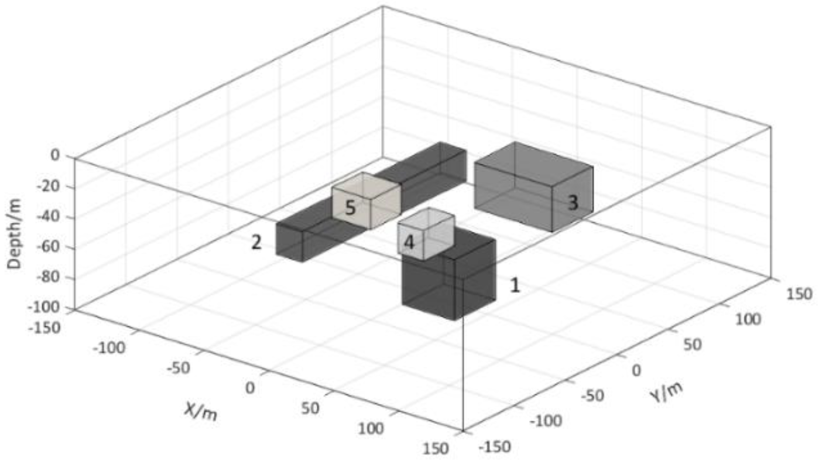
The synthetic model consisted of five cuboids with different space sizes, properties, and depths. The distance between survey points and survey lines was 1 m. The model’s spatial distribution is shown in Figure 3.

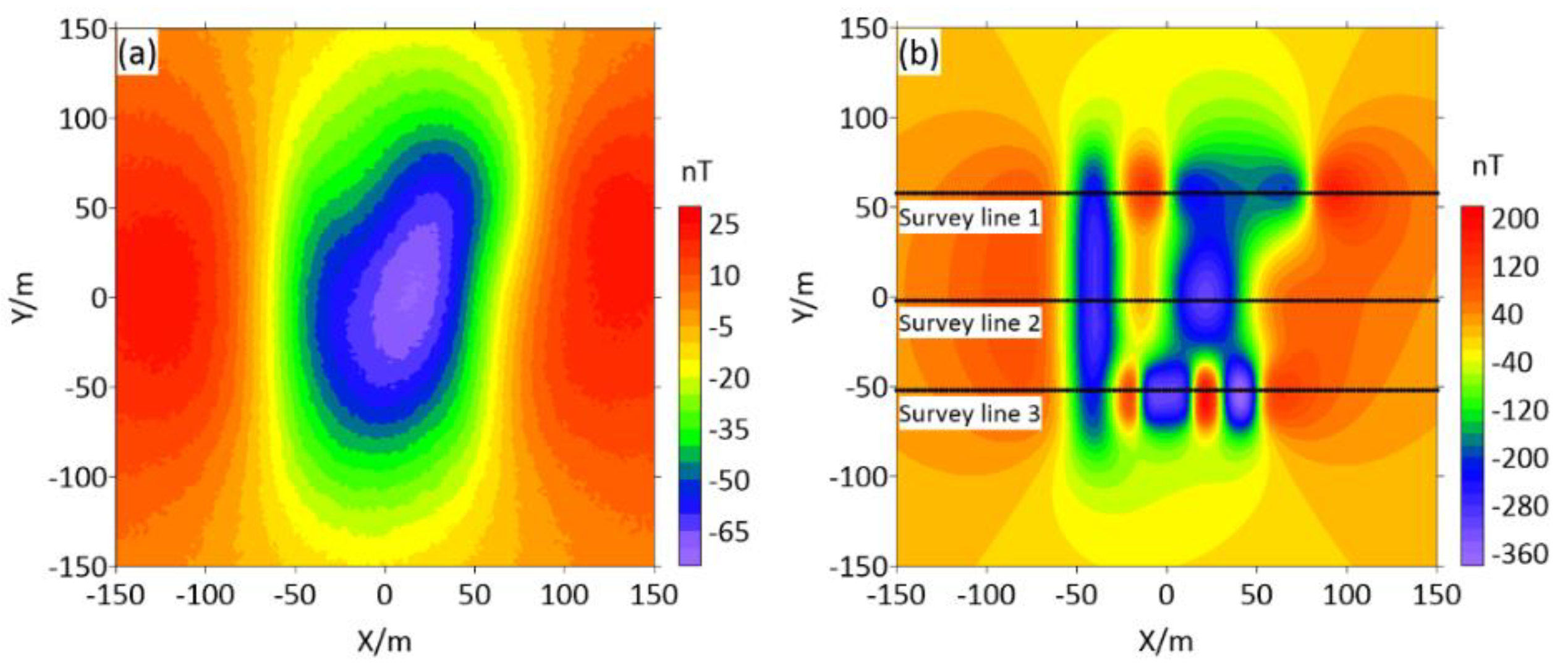
Figure 4 shows the magnetic data induced by the above model measured at different heights, of which the magnetic data (in Figure 4a) measured at 40 m was used as the initial magnetic field for downward continuation. An accurate downward continuation of this data to 0 m should correspond well to the theoretical magnetic data, as seen in Figure 4b. Further, the magnetic data at 40 m contained Gaussian random noise with standard deviation of 5% of the maximum data amplitude. This noisy data could be applied to test the stability of the downward continuation method. In this test, two other methods, including the wave number domain iterative method and the unconstrained equivalent source downward continuation method, were also performed for comparison.

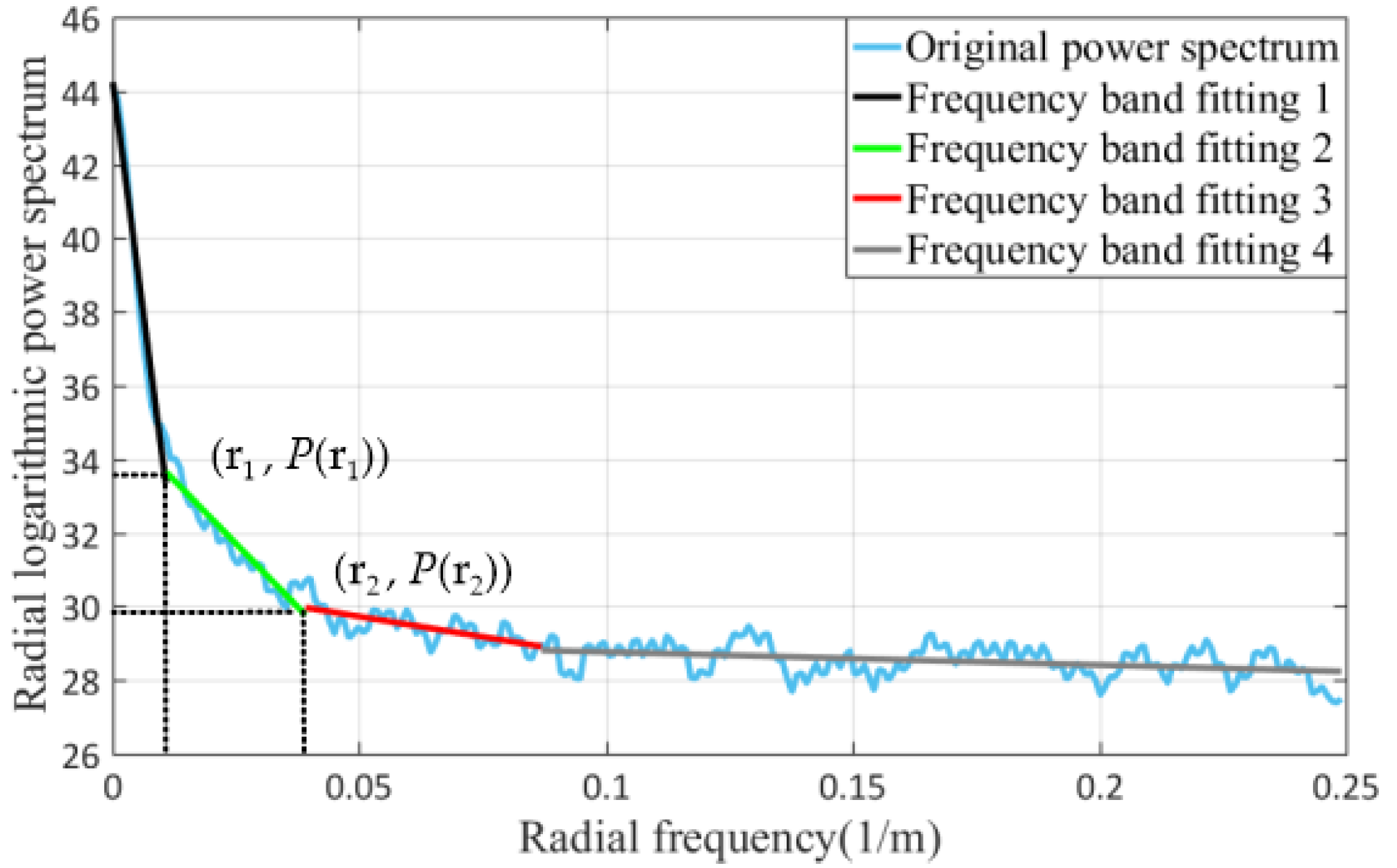
The equivalent source depth could be estimated by analyzing the radial logarithmic power spectrum (Figure 5). In this model test, the radially averaged logarithmic power spectrum was divided into four segments for piecewise fitting. Each fitting line represents a depth that can be estimated by Equation (20) [24]:

$$h=\frac{P(r_1)-P(r_2)}{4\pi (r_2-r_1)}$$

(20)

where $r_1$ and $r_2$ are the start and end radial frequency of the fitting line, respectively, and $p(r_1)$ and $p(r_2)$ are the corresponding radial power. We chose the depth represented by the black line that was the deepest; correspondingly, $r_1=0$, $p(r_1)=44.21$, $r_2=0.012$ and $p(r_2)=33.91$. Then, following Equation (20) the result was 80.61 m. After that, the equivalent source was set at this depth. The lower space at this depth was divided into 200 × 200 cube cells, and each cell size was 1 m × 1 m × 5 m.

The theoretical magnetic data (Figure 4a) were utilized to invert the susceptibility parameters of the equivalent source, and the measured data from three survey lines, as Figure 4b shows, were used as constraint data in the inversion process.

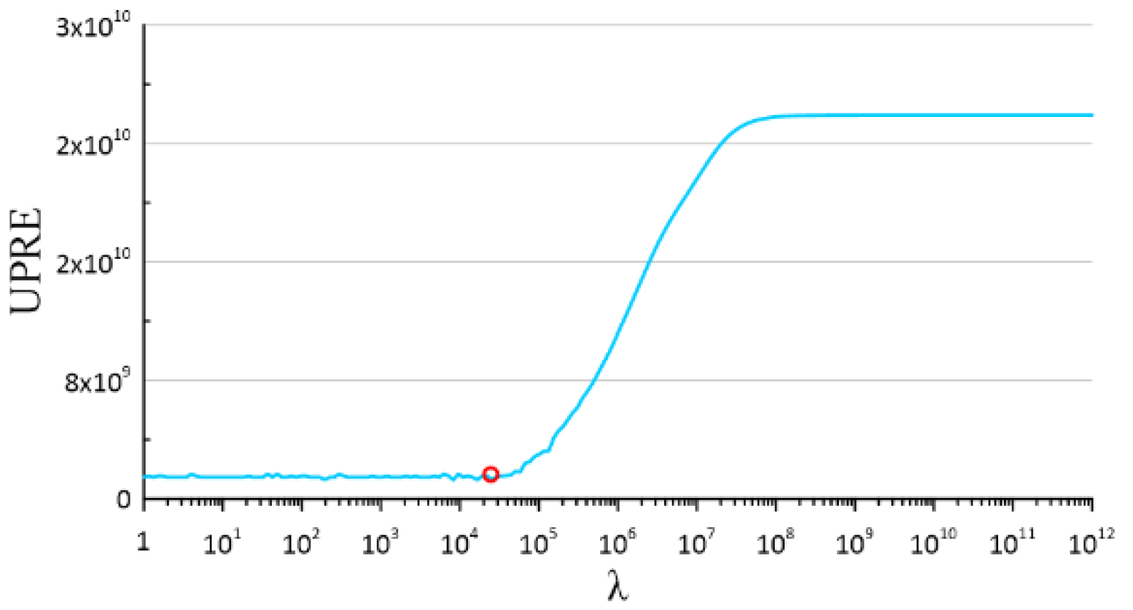
According to Equation (12), the regularization parameter λ is obtained by the UPRE function, and the relationship of λ and value of Equation (12) is the blue line in Figure 6; furthermore, the red circle is the minimum value of UPRE, and therefore we chose the corresponding value (λ = 8309.94) to solve Equation (13).

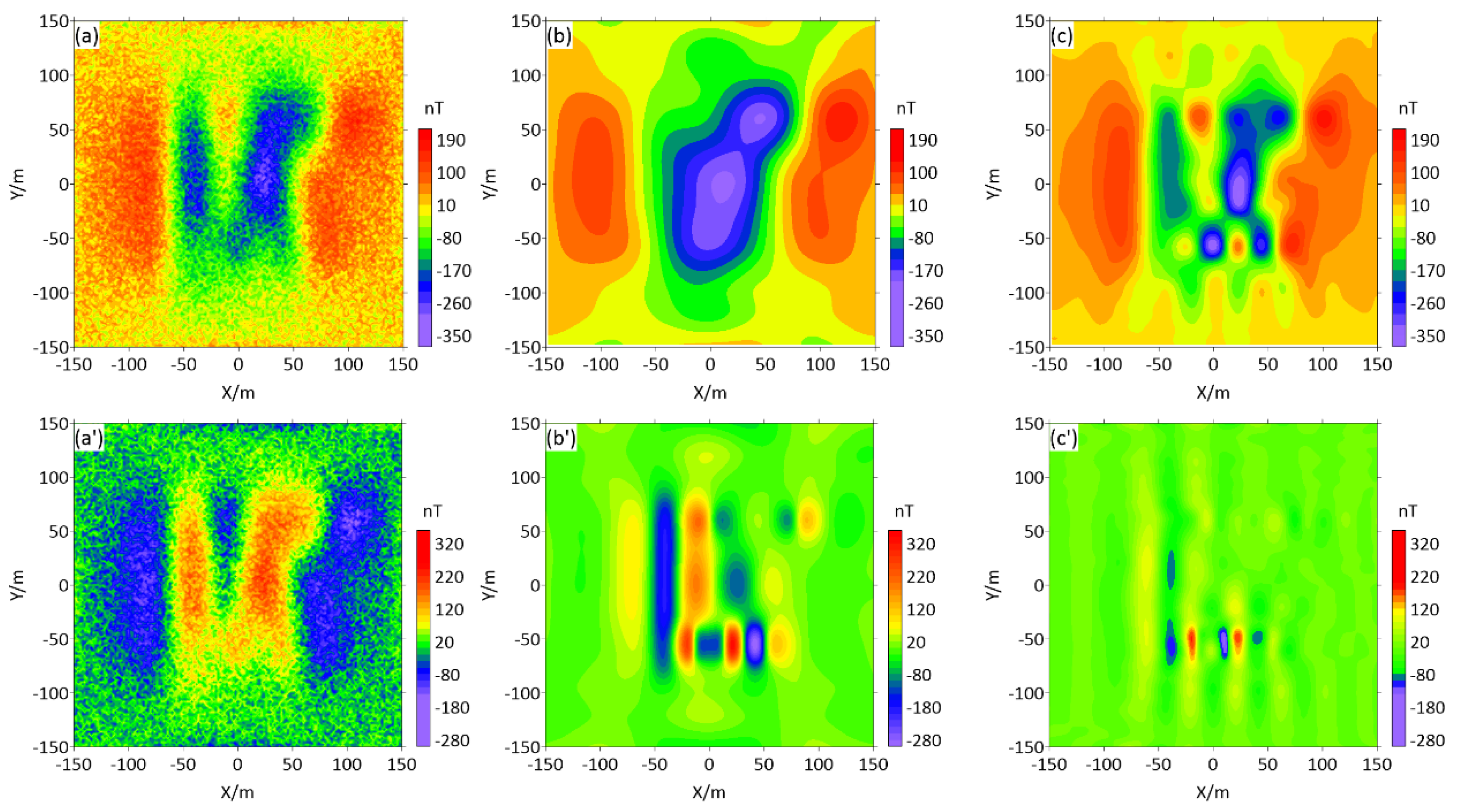
Finally, we followed Equation (19) to forward calculate the magnetic anomaly at the depth of 40 m under the 0 m observation surface. The equivalent source method and wave number domain iteration method were used for downward continuation of the same distance for comparison.

The results for those methods are shown as Figure 7. When the continuation was conducted with large distance, according to Figure 7a, the wave number domain iterative method was disturbed by noise seriously, which led to a huge misfit. The result of the equivalent source method (Figure 7b) had a similar amplitude to the theoretical value, yet the amount of information missed and the abnormal trend were different. The result of the constrained equivalent source method (Figure 7c) was closer to the theoretical value of the anomaly shape and amplitude than others, and also had good noise suppression. The deviation diagrams (Figure 7a’,c’,b’) were obtained by applying theoretical data (Figure 4b) minus the results of different methods, and from that they could be illustrated more intuitively. The deviation of the constrained equivalent source method was minimal, and the high value deviations in other two methods were counterbalanced.

The quantitative comparison of each method resulted in differences with the theoretical magnetic data, as

Table 2. The difference between the results of the downward continuation methods and the theoretical magnetic data.

Method	Maximum (nT)	Minimum (nT)	Mean (nT)	RMSE (nT)
Wave number domain iteration	357.220	−273.520	−1.018	46.768
Equivalent source	333.511	−296.890	0.151	52.125
Constrained equivalent source	198.991	−149.11	0.083	29.459

shows, which demonstrated that the constraint equivalent source method improves the accuracy.

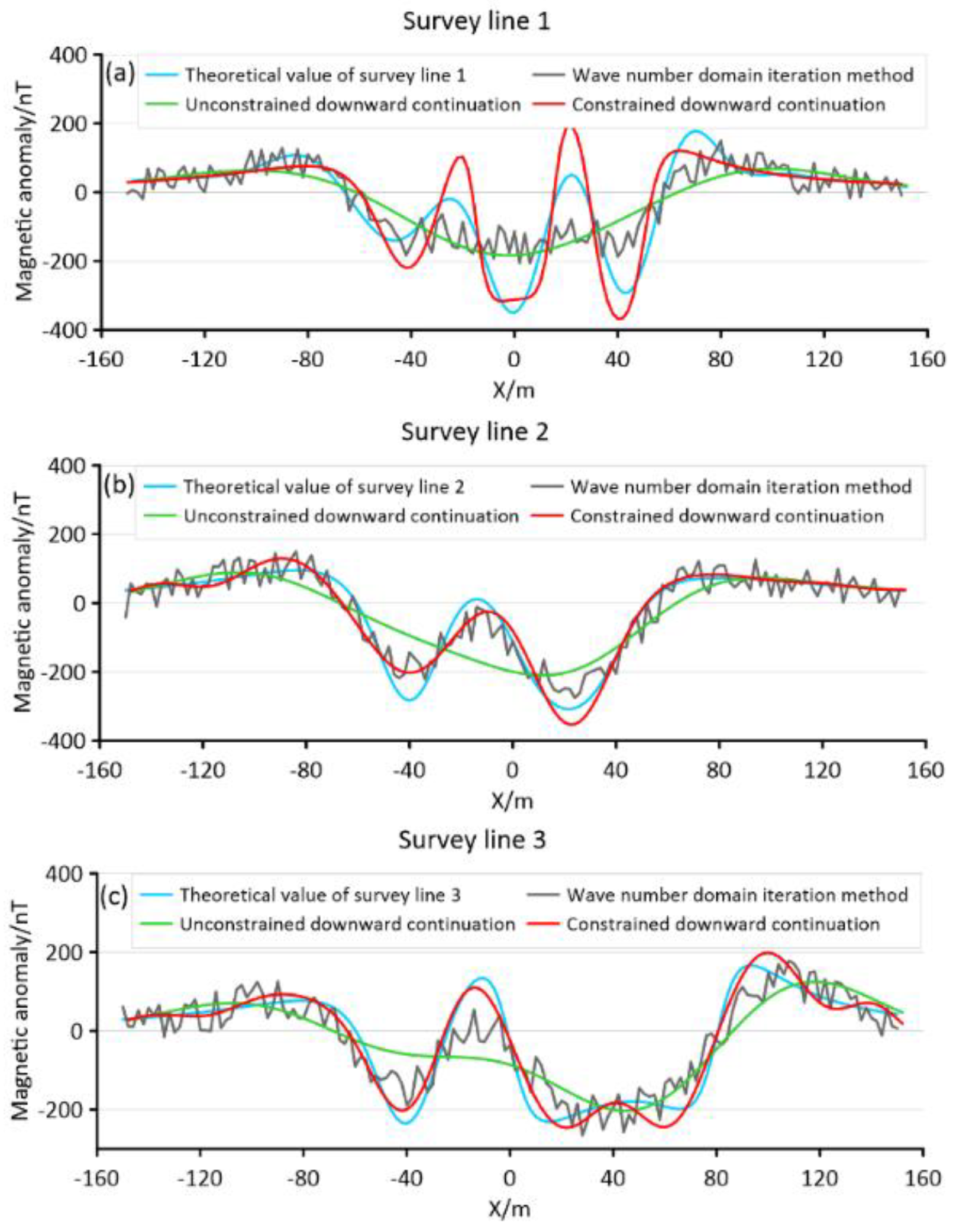
According to Figure 8, we extracting the data corresponding to the survey lines position (shown as Figure 4b) from the results of the three downward continuation methods, it could be clearly seen that the result of the wavenumber domain iteration method (the black line) deviated greatly from the theoretical value (the blue line) due to the influence of noise. The constrained equivalent source method (the red line) could fit the theoretical value well, and the influence of noise was relatively minimal.

4. Application to Measured Magnetic Data

To further investigate the effectiveness of the constrained strategy, an example from the South China Sea Area was presented. Specifically, the data acquisition ship was the “Ocean No. 6” multifunctional geological and geophysical survey ship affiliated with the Guangzhou Marine Geological Survey, equipped with a deep-water gravity and magnetic exploration system with underwater automatic depth determination and attitude control functions.

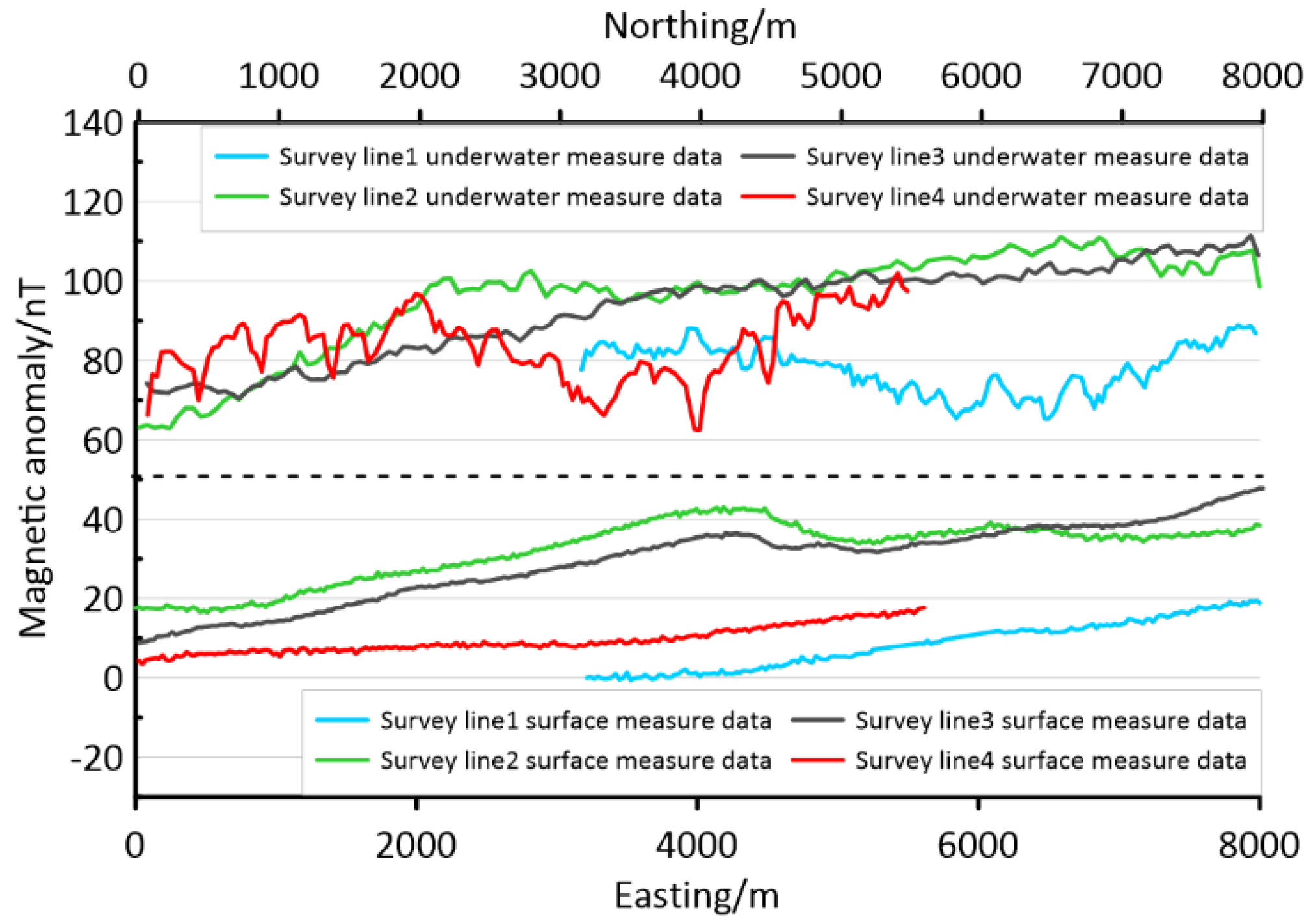
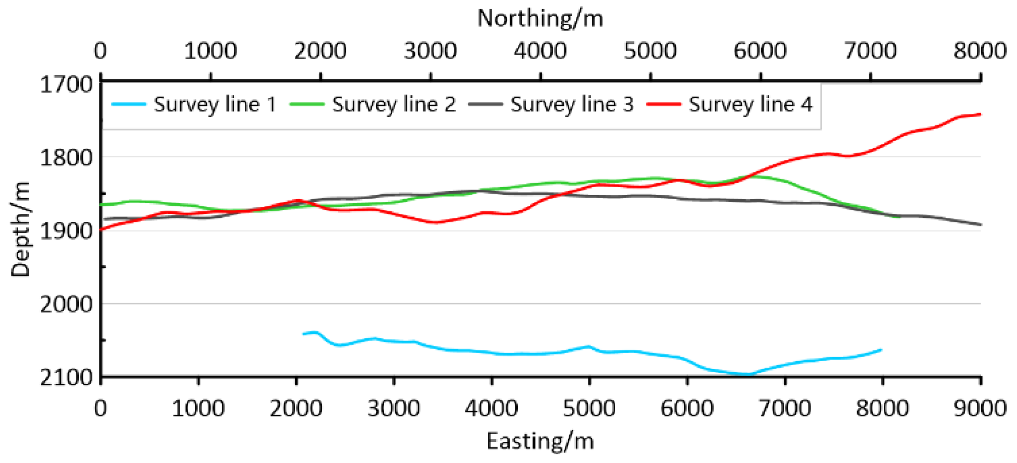
This system was used to measure the magnetic anomalies of eight survey lines corresponding to each other on the sea surface and underwater. The measured magnetic data of each survey line are shown in Figure 9, and the corresponding depth of four underwater survey lines are shown in Figure 10.

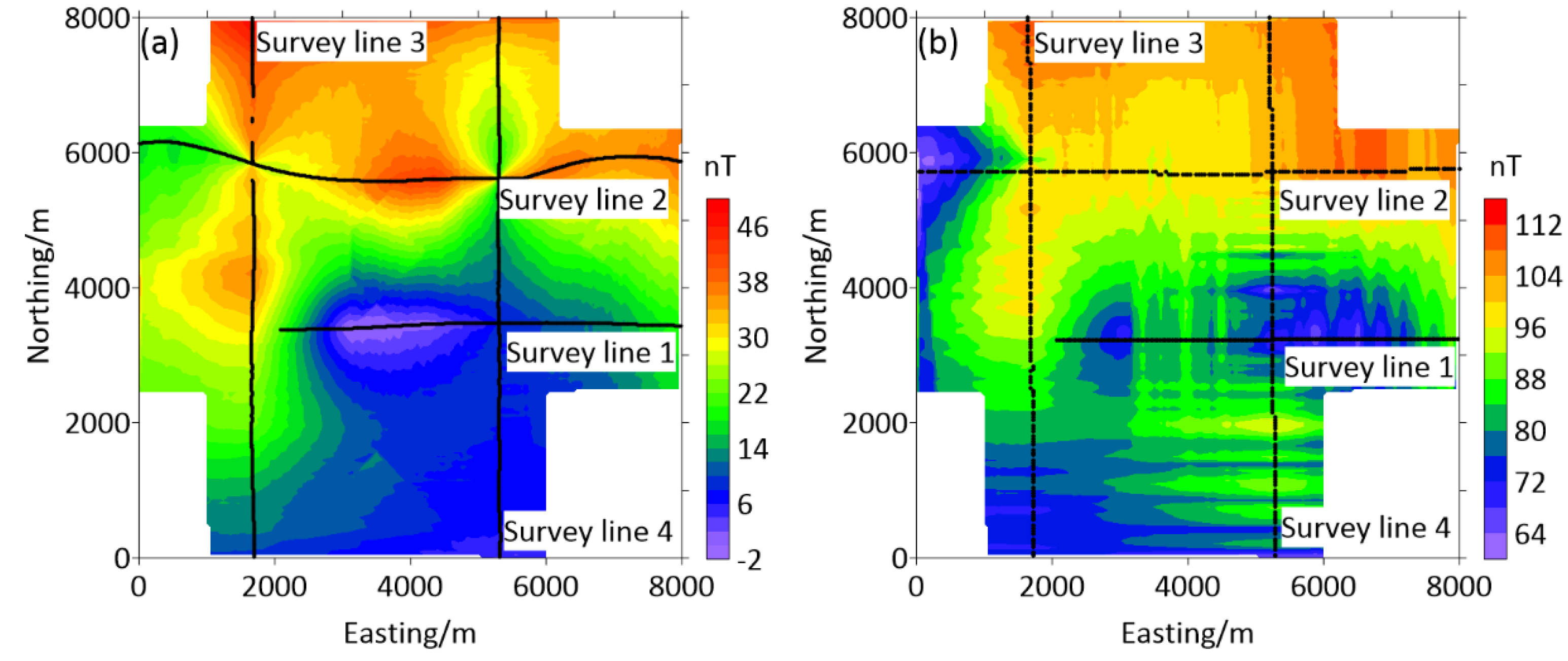
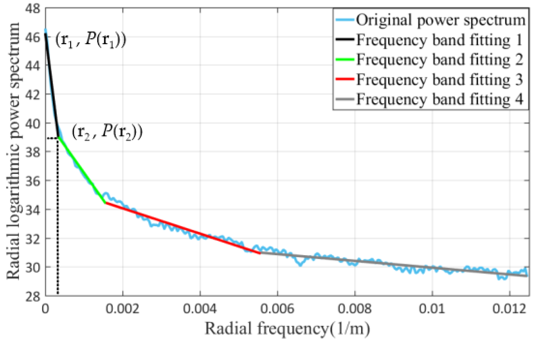
The surface and underwater measured data were interpolated into a regular grid, as shown in Figure 11. The radially averaged logarithmic power spectrum of sea surface measured data is shown in Figure 12, divided into four segments for piecewise fitting. Equation (20) was used to estimate the depth of each frequency band, and in this paper, the deepest depth of 2706.8 m (the black line) was set as the equivalent layer depth, where $p(r_1)=46.13$, $r_2=0.00021$, and $p(r_2)=39.02$. Eventually, the lower space of this depth was divided into 400 × 400 cube cells, and each cell size was 1 × 1 × 5 m.

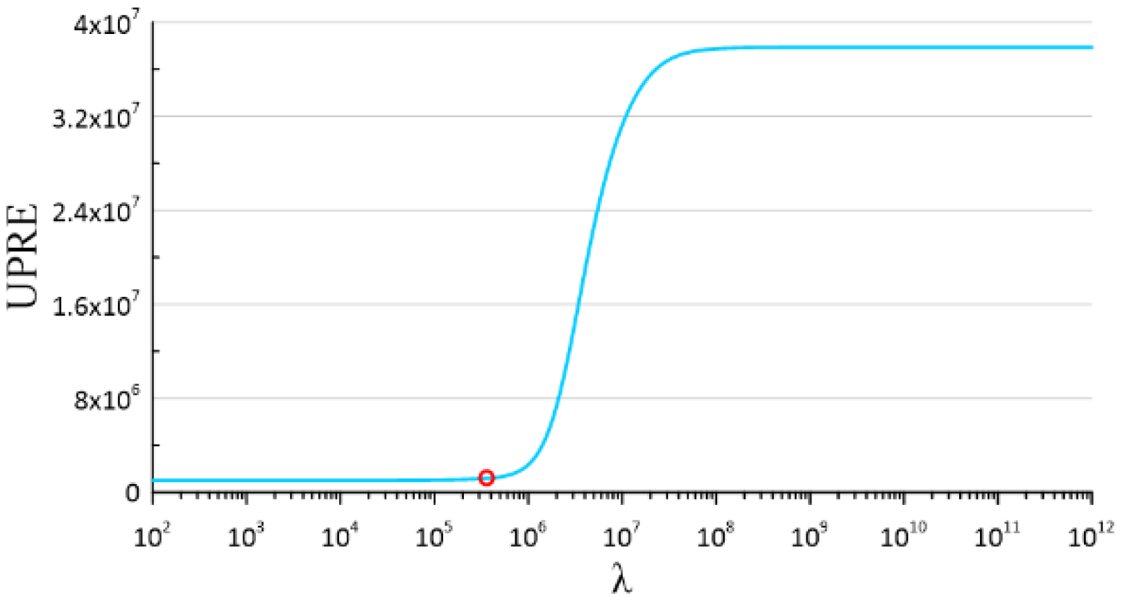
According to Equation (14), the regularization parameter λ is obtained by the UPRE function, and the relationship of λ and value of Equation (14) is the blue line in Figure 13; furthermore, the red circle is the minimum value of UPRE, and therefore we chose the corresponding value of λ to solve Equation (15).

Then, the equivalent layer forward modeling results were used to fit the measured magnetic anomalies on the sea surface to obtain the equivalent source parameters, and finally the water surface magnetic (Figure 11a) anomaly was determined to be downward continuation by the wave number domain iteration method, the unconstrained equivalent source method, and the constrained equivalent source method, respectively. 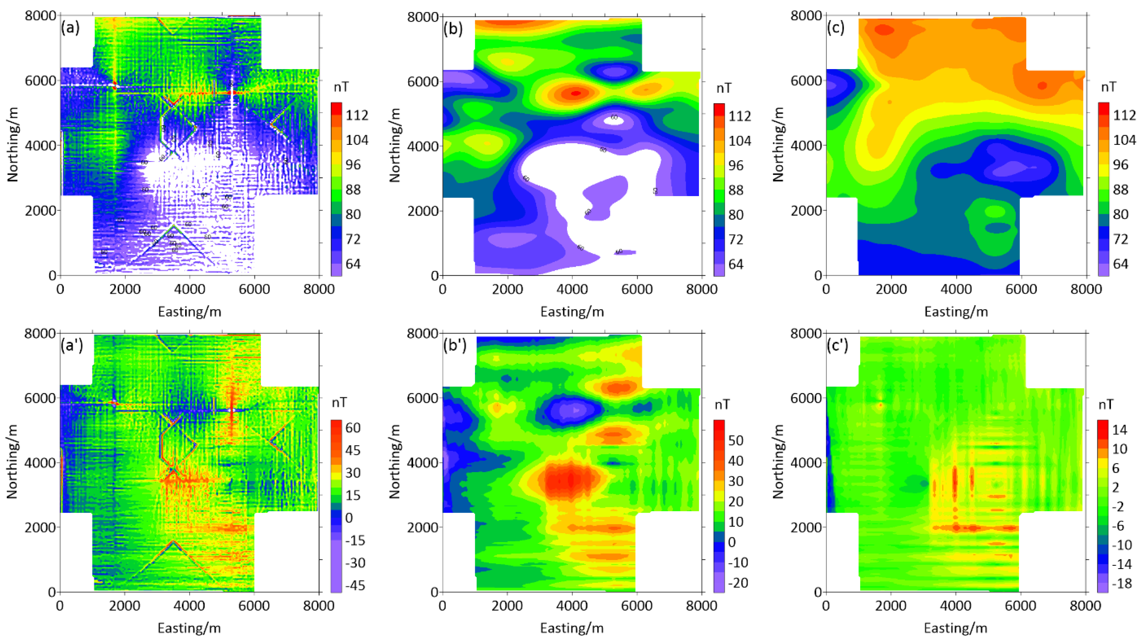The constrained data were the four underwater survey lines data, and as Figure 11b shows, the result of downward continuation amplitude was set up to be consistent with the range of the measured value and then was compared with the underwater measured data, as Figure 14 shows.

It can be seen from Figure 14a that the noise was inevitably amplified when this method was downward continuation over a long distance, which affected its accuracy, and the abnormal trend was quite different from the measured data (Figure 11b). The result of the unconstrained equivalent source method (Figure 14b) showed an abnormal shape similar to the measured data, but its amplitude was smaller than the measured value. The abnormal shape more reflected the trend and lacked some detailed information compared with the measured value. The result of the constrained equivalent source method (Figure 14c) obtained both anomalous shape and amplitude, similar to the measured value, and the noise effect was small and also contained detailed information.

According to the deviation diagram (Figure 14a’,c’,b’), these results can be more clearly. The deviation of the constrained equivalent source method was minimal, and it not only overcame the effect of noise, as Figure 4a’ shows, but also counterbalanced the high value deviation, as Figure 4b’ depicts.

The quantitative comparison of each method showed different results with measured magnetic data at a depth of 2000 m under the sea surface, as

Table 3. The difference between the result of downward continuation methods and the measured magnetic data at depth of 2000 m under the sea surface.

Method	Maximum (nT)	Minimum (nT)	Mean (nT)	RMSE (nT)
Wave number domain iteration	314.753	−194.68	29.610	17.048
Equivalent source	108.085	−58.626	15.179	14.783
Constrained equivalent source	108.084	−51.335	1.482	11.758

shows. Obviously, the proposed method reduced the average deviation and obtains the lowest RMSE, which demonstrated that the result of this method had high accuracy.

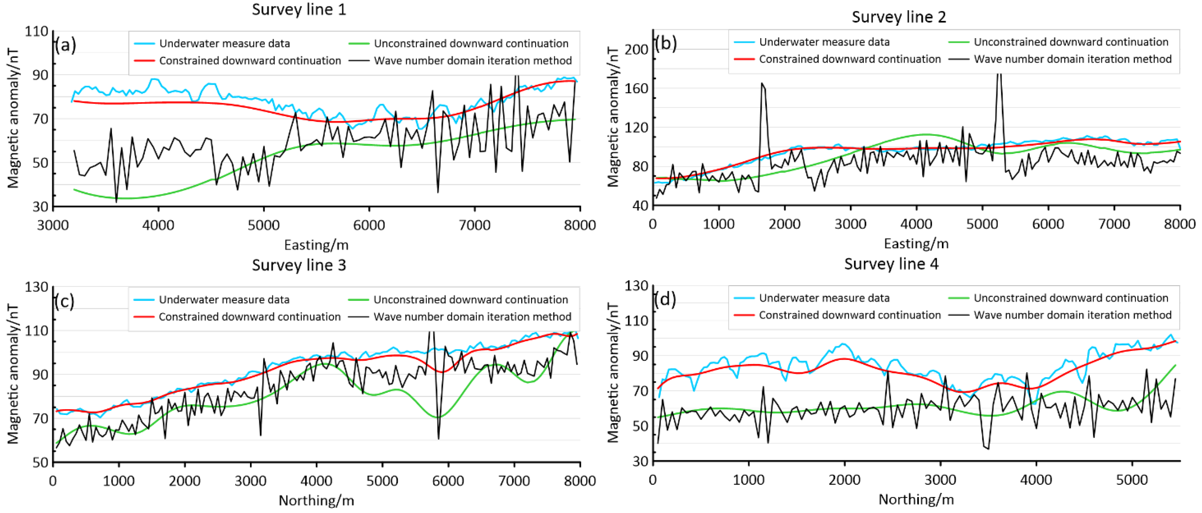
The magnetic anomaly values corresponding to the positions of the four underwater survey lines in the continuation results of the three methods were extracted and then compared with the actual measured values, as shown in Figure 15. Intuitively, the abnormal trend of the wave number domain iteration method (the black line) was similar to the measured value (the blue line); however, there were amplitude oscillations due to the noise. The results of the unconstrained equivalent source method (the green line) continuation were less affected by noise, and the range of amplitude variation and the abnormal shape and trend were similar to the measure data, but the amplitude had a relative huge misfit with the measure data. Compared with the previous two methods, the constrained equivalent source method (the red line) continuation value was closer to the measure data. The range of amplitude and the abnormal shape could fit the measured value properly. The constructed equivalent source could reflect more attenuated high-frequency information in the continuation results due to the data of the underwater survey lines being added as constraints. Figure 15 shows that the continuation results of the unconstrained equivalent source method (the green line) lost much information, which was reflected in the measured data, but it was recovered after adding constrained data.

5. Conclusions

In this paper we introduce a constrained equivalent source downward continuation scheme to achieve the long-distance stable downward continuation, which overcomes the amplitude attenuation effect and recovers the lost deep high-frequency signal. We obtain the solution by minimizing a specific objective function of the model that integrates the lower space measured data. When the downward continuation distance is too large, the high frequency potential field information generated by the magnetization anomaly in the underground space is seriously attenuated and difficult to reflect on the observation surface. Therefore, whether it is to use the filter operator to amplify signal or the equivalent source to construct the forward model, the result would deviate from the true value. The method proposed in this paper takes the actual measured value of the underground space as the constraint data and constrains it during the process of calculating the equivalent source model parameters, so that the final continuation result is close to the true value, and it is used in the model test and actual data processing, both obtain a good fitting performance.

However, the number of subdivision cells in the underground space will also directly affect the continuation accuracy. Theoretically, the finer the subdivision cells are, the higher the accuracy is, but this would increase the amount of calculation. Subsequent studies will be focused on how to refine the division as much as possible. Researching a balance between more equivalent cells and satisfying the calculation speed makes this method more accurate and efficient.