Article

Forecasting the Daily Maximal and Minimal Temperatures from Radiosonde Measurements Using Neural Networks

Faculty of Mathematics and Physics, University of Ljubljana, Jadranska 19, 1000 Ljubljana, Slovenia
*
Author to whom correspondence should be addressed.
Appl. Sci. 2021, 11(22), 10852; https://doi.org/10.3390/app112210852
Submission received: 24 September 2021 / Revised: 27 October 2021 / Accepted: 10 November 2021 / Published: 17 November 2021
(This article belongs to the Special Issue Applications of Machine Learning on Earth Sciences)

Abstract

:
This study investigates the potential of direct prediction of daily extremes of temperature at 2 m from a vertical profile measurement using neural networks (NNs). The analysis is based on 3800 daily profiles measured in the period 2004–2019. Various setups of dense sequential NNs are trained to predict the daily extremes at different lead times ranging from 0 to 500 days into the future. The short- to medium-range forecasts rely mainly on the profile data from the lowest layer—mostly on the temperature in the lowest 1 km. For the long-range forecasts (e.g., 100 days), the NN relies on the data from the whole troposphere. The error increases with forecast lead time, but at the same time, it exhibits periodic behavior for long lead times. The NN forecast beats the persistence forecast but becomes worse than the climatological forecast on day two or three. The forecast slightly improves when the previous-day measurements of temperature extremes are added as a predictor. The best forecast is obtained when the climatological value is added as well, with the biggest improvement in the long-term range where the error is constrained to the climatological forecast error.

1. Introduction

The meteorological community is increasingly using modern machine learning (ML) techniques to improve specific aspects of weather prediction. It is conceivable that someday the data-driven approach will beat the numerical weather prediction (NWP) using the laws of physics, although several fundamental breakthroughs are needed before this goal comes into reach [1,2,3]. So far, the ML was mostly used to improve or substitute specific parts of the NWP workflow. For example, neural networks (NNs) were applied to describe physical processes instead of individual parametrizations [4,5,6], and to replace parts of the data assimilation algorithms [7]. NNs were also used to downscale the low-resolution NWP outputs [8], or to postprocess ensemble temperature forecasts to surface stations [9], whereas Grönquist et al. [10] used them to improve quantification of forecast uncertainty and bias. In several studies, ML methods were utilized for the data analysis, e.g., detection of weather systems [11,12] and extreme weather [13]. ML methods were also applied to emulate the NWP simulations using NNs trained on reanalyses [14,15,16,17] or simulations with simplified general circulation models [18]. Thus far, not many attempts were made at constructing end-to-end workflows, i.e., taking the observations as an input and generating an end-user forecast [3]. Some examples of such approaches are Jiang et al. [19], which tried to predict wind speed and power, and Grover et al. [20], which attempted to predict multiple weather variables from the data of the US weather balloon network. The NNs were shown to be particularly successful in precipitation nowcasting. For example, Ravuri et al. [21] used radar data to perform short-range probabilistic predictions of precipitation, while Sønderby et al. [22] combined radar data with the satellite data.
Here we attempt to develop a model based on the NN that takes a single vertical profile measurement from the weather balloon as an input and tries to forecast the daily maximum ( T max ) and minimum ( T min ) temperatures at 2 m at the adjacent location for the following days. The aim of this work is not to develop an approach that would be better than the current state-of-the-art NWP models. Since only a single vertical profile measurement is used, it could hardly be expected that the NN model could perform better than an operational NWP model (which uses a fully fledged data assimilation system incorporating measurements of the global observation network). Our goal is rather to explore the capability of neural networks for these kinds of forecasts. More specifically, our aim was to understand how the NN-based models utilize different types of input data and how the network design influences their behavior. The data utilization and behavior of the network will be different whether the NNs are used for short- or long-term forecasts—this is why the analysis was performed for a wide range of forecast lead times going from 0 to 500 days into the future. By studying these networks, we hoped to gain some valuable insights that might help others develop more complex setups and neural-network-based data assimilation schemes.
Section 2 presents the data and the methodology. Section 3 presents an analysis based on very simple NNs, consisting of only a few neurons, while Section 4 describes the analysis based on more complex NNs used for short- and long-term forecasts. Discussion and conclusions are given in Section 5.

2. Data and Methods

2.1. Data

Vertical profiles from radiosonde measurements and measurements of maximum and minimum daily temperatures were used in the analysis. Each dataset is described in more detail below.

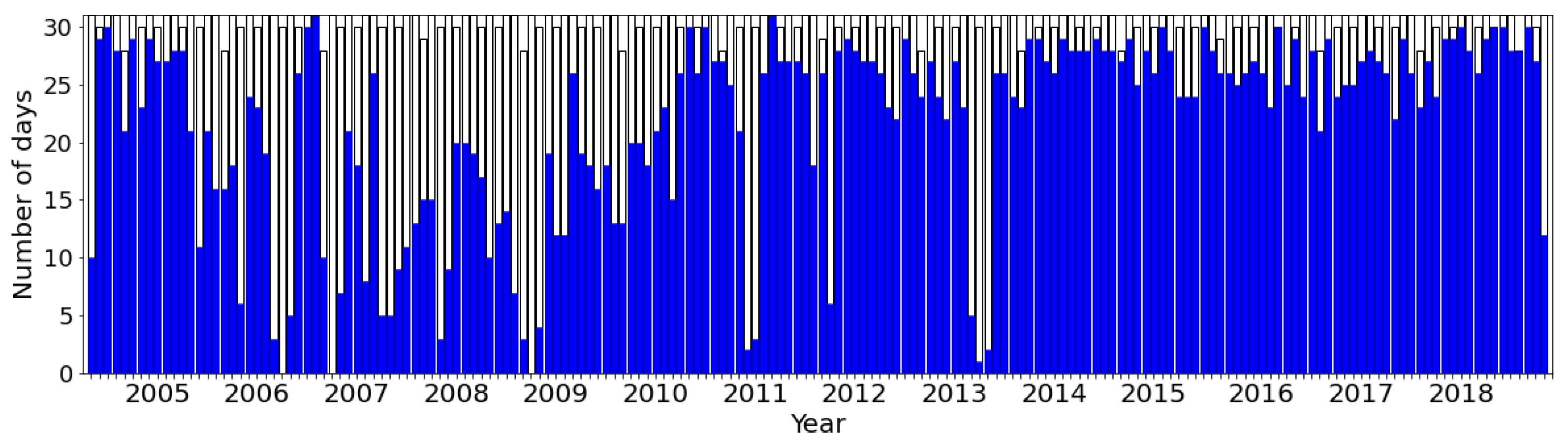
2.1.1. Radiosonde Measurements

The vertical profile data were obtained from the radiosonde measurements. A radiosonde is an expendable meteorological instrument package, often borne aloft by a free-flight balloon, that measures, from the surface to the stratosphere, the vertical profiles of atmospheric variables and transmits the data via radio to a ground receiving system [23]. The radiosondes are operated by the Slovenian Environment Agency (SEA). They are launched once per day from the Ljubljana-Bežigrad station that is part of the SEA observation network (altitude 299 m, longitude 14.5124°, latitude 46.0655°). The set of data contains 4420 vertical profiles from October 2004 to May 2019. Each vertical profile consist of measurements of seven variables: altitude (z), temperature (T), dew-point temperature ( T d ), relative humidity ( R H ), pressure (p), wind speed ( | v | ) and wind direction ( θ ).
The radiosondes can ascend to an altitude exceeding 25 km; however, oftentimes, the maximal altitude reached by radiosonde is significantly lower. To homogenize the data and not exclude too many measurements, we decided only to use data below 12 km for the analysis (this at least guarantees that the whole troposphere is included in the measurements). Quality control was performed to remove the profiles that contained non-realistic values or missing data. We excluded all profiles that met any of the following criteria: (i) the altitude of the lowest measurements is larger than 299 m (the altitude of the Ljubljana-Bežigrad station), (ii) the altitude of the highest measurement is smaller than 12 km, (iii) there exists a vertical gap without measurements that is larger than 100 m, (iv) the relative humidity of the lowest measurement is smaller than 10%, (v) the temperature of the lowest measurement is smaller than −35 °C and (vi) there is at least one non-numeric value present (e.g., infinite, not a number) in the measurements. Thus the final set that was used for the analysis contained only 3800 profiles. The majority of days without measurements are before 2011, as shown in Figure 1. The measurements were performed in the early morning hours: 46.8% of measurements were performed at 03 UTC, 41.7% at 04 UTC, 10.3% at 02 UTC, and the remaining at other times.
During the ascent, the radiosonde performs measurements every second, and the typical vertical resolution of the profile measurement is about 5 m. The vertical speed of the radiosonde depends on various meteorological parameters as well as the amount of helium in the balloon. Thus, the rate of ascent can be slightly different each day, and the altitudes at which the radiosonde records a measurement are also different. Further, the values of the measured meteorological parameters typically do not change much in 5 m, so it makes sense to use a coarser vertical resolution; therefore, we decided to interpolate the vertical measurements to 118 predefined altitude levels at every 100 m, with the lowest level being at 300 m and the highest one at 12 km (linear interpolation was used).

2.1.2. Daily Maximum and Minimum Temperature

The daily maximum and minimum temperatures at 2 m ( T max and T min ) were measured at the same station from which the radiosonde is launched (i.e., Ljubljana-Bežigrad station). The data were available for the same period as the radiosonde data and were without any missing data. The daily minimum typically occurs early in the morning, sometime after sunrise, while the daily maximum temperature is generally observed in mid-afternoon; however, the minimums and maximums can occasionally also occur at other times, e.g., if the frontal system passes the station during the day.
We also calculated the daily climatological values for the T max and T min . The climatological values were computed as average values in a 7-day window centered on a specific day in the period 2000–2020. For example, the value corresponding to June 5th is the average value of T max or T min in days between June 2nd and June 8th in the period 2000–2020.
Figure 2 shows the correlations of the vertical profiles of temperature, dew-point temperature and relative humidity with measurements of daily maximum and minimum temperature performed on the same day. As could be expected, the correlations are high for radiosonde temperatures near the ground, with correlations starting to noticeably decrease above the altitude of 1.2 km, although they are larger than 0.6 in most of the troposphere, while they rapidly decrease in the stratosphere. The correlations near the ground are also large for dew-point temperature but start to decrease much more rapidly with altitude. For relative humidity, the correlations are generally low. For T max , the correlations with R H are weakly negative in most of the troposphere, which could be linked to the possible existence of clouds that weaken downward shortwave radiation near the ground during the day, which reduces the temperature. For T min the correlations with R H are weakly positive, which could be linked to clouds and high humidity causing an increase of downward longwave radiation near the ground during the night, which decreases the night-time radiation cooling and thus causes an increase in temperature.
Note that T, T d and R H are related via the following equation (derived from Clausius–Clapeyron relation):
log R H = L R v 1 T 1 T d
and thus they are not independent (uncorrelated) variables. In Equation (1), L = 2.5 MJ kg 1 denotes latent heat of condensation, while R v = 461.5 J kg 1 K 1 is the specific gas constant for water vapor.
Previous-day temperature extremes, T max ( t 1 ) and T min ( t 1 ) , show very high correlation (correlation coefficient 0.95) with present-day extremes, T max ( t ) and T min ( t ) , while the correlation with the same-day climatological extremes is approximately 0.9.

2.2. Methods

2.2.1. Neural Network Setup

All the setups consisted of a dense sequential network, where the nearby layers are fully interconnected (each neuron in a specific layer is connected to every neuron in the next layer). We used Keras and Tensorflow libraries [24] in Python to set up and train the NNs. While the NN design and the number of input variables were different for every setup (these are described in detail in the following sections), the output was always the same—a single forecasted value of either T max or T min . The training was performed separately for each forecast lead time (the lead time was not used as a predictor). For example, the network for the 10-day forecast was trained independently of the network for the 100-day forecast. Thus each NN could focus on improving the performance at only one lead time, without heaving to worry about other lead times.
To thoroughly analyze the behavior of each NN setup, we performed 50 realizations of the network training for every setup and thereby obtained an ensemble of NN models for each lead time. Due to random initialization of weights, each training produces a somewhat different NN, even though the network setup is the same and the NN is trained on the same data. Out of all available cases (3800 days), we used 90% for training and validation (of these 70% were used for training and 30% for validation), and the remaining 10% for testing. The 380 days in the testing set were selected randomly. The same set of testing cases was used to evaluate the performance of all setups and every training realization. Since the same test cases were used the comparison of performance of different setups and training realizations is more meaningful (as opposed to each setup using a different test set). Before the training, all the input data were scaled using the MinMaxScaler function from the Scikit-learn library [25], which normalized the input variables to the range from 0 to 1 (the normalization was performed separately for each input variable). For the training, we used Adam optimizer along with the mean absolute error metric (MAE, [26]) for the loss function. We experimented with the values for various hyperparameters such as batch size, number of epochs, activation functions and learning rate reduction (described in the following sections). Figure 3 shows an example of NN training.

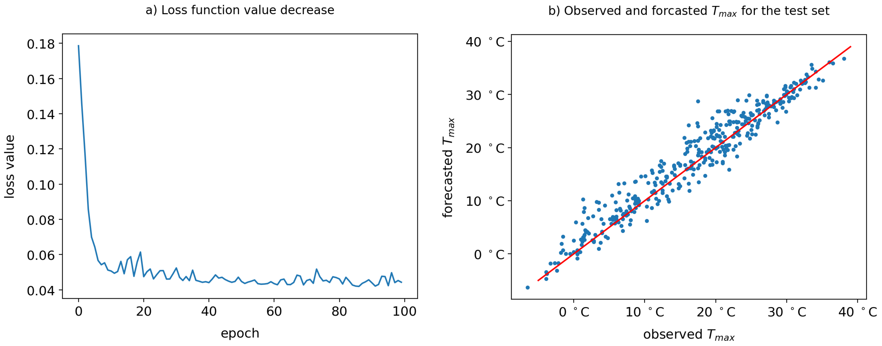
2.2.2. Forecast Performance Evaluation

The performance of the NN forecasts was evaluated on the test set using the MAE metric. Since we had an ensemble of NN models, we obtained a distribution of MAE values for every setup. We could calculate various statistical parameters from these distributions, such as the average value and the 10th and 90th percentile of MAE.
The performance of the NN forecasts was also compared to the persistence and climatological forecasts. The persistence forecast assumes that the value of T max or T min for the next day (or any other day in the future) will be the same as the previous day’s value. The climatological forecast assumes the value for the next day (or any other day in the future) will be identical to the climatological value for that day in the year (the calculation of climatological values is described is Section 2.1.2).

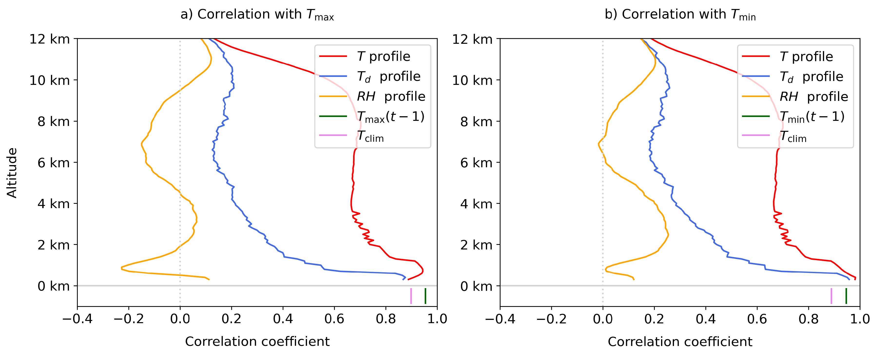
2.2.3. Neural Network Interpretation

We also used two simple but effective explainable artificial intelligence (XAI) methods [27], which can be used to interpret or explain some aspects of NN model behavior.
The first was the input gradient method [28], which calculates the partial derivatives of the NN model with respect to the input variables. If the absolute value of derivative for a particular variable is large (compared to the derivatives of other variables), then the input variable has a large influence on the output value; however, since the partial derivative is calculated for a particular combination of values of the input variables, the results cannot be generalized for other combinations of input values. For example, if the NN model behaves very nonlinearly with respect to a particular input variable, the derivative might change significantly depending on the value of the variable.
This is why we also used a second method, which calculates the span of possible output values. The span represents the difference between the maximal and minimal output value as the value of a particular (normalized) input variable gradually increases from 0 to 1 (we used a step of 0.05), while the values of other variables are held constant. Thus the method always yields positive values. If the span is small (compared to the spans linked to other variables) then the influence of this particular variable is small. Since the whole range of possible input values between 0 and 1 is analyzed, the results are somewhat more general compared to the input gradient method (although the values of other variables are still held constant).
The problem for both methods is that the results are only valid for specific combinations of input values. This issue can be partially mitigated if the methods are applied to a large set of input cases with different combinations of input values. Here we calculated the results for all the cases in the test set and averaged the results. We also averaged the results over all 50 realizations of training for a specific NN setup—thus the results represent a more general behavior of the setup and are not limited to a particular realization.

3. Simplistic Sequential Networks

This section presents an analysis based on very simple NNs, consisting of only a few neurons. The goal was to illustrate how the nonlinear behavior of the NN increases with network complexity. We also wanted to determine how different training realizations of the same network can result in different behaviors of the NN.
The NN is basically a function that takes a certain number of input parameters and produces a predefined number of output values. In our case the NN is a scalar function since it always outputs a single value (i.e., either T max or T min ). Since we wanted to illustrate the NN behavior we limited the number of input parameters to two—this enabled us to visually show the behavior of the NN as 2D contour graph. We aimed to try out various setups of simplistic NNs, with different degrees of complexity and see how it affects the resulting behavior.
We focused on the same-day forecast (forecast for the same day as the radiosonde measurement was made). We wanted to use two profile-based input parameters that would produce a reasonably good forecast of either T max or T min . We experimented with various parameters derived from the vertical profiles. In the end, we chose the average temperature in the lowest layer between the ground and 1 km and the 90th percentile of RH in the layer between the ground and 12 km (both parameters were calculated from the data of the original profiles, without interpolation to standard altitudes). The first parameter reflects the general temperature conditions in the boundary layer, which will depend on the season and also the general weather situation (the strong link between T max and the temperature in the boundary layer is also clearly visible in Figure 2). The second parameter can be associated with the existence of cloudiness. As already mentioned, the clouds will weaken downward shortwave radiation near the ground during the day, which reduces the temperature near the surface. The radiosonde does not directly measure the existence of clouds. Still, it can be approximately inferred from the RH measurements (an RH value larger than 90% indicates a high likelihood of clouds at that altitude). Besides the possibility of either having none or at least some clouds, the cloud thickness also influences the downward shortwave radiation. If there are no clouds, the 90th percentile of RH will have a relatively low value (i.e., significantly smaller than 100%), whereas if a sufficiently thick cloud layer is present, the 90th percentile of RH will be close to 100%.
The analyzed NN setups are described in Table 1. We started with the most simple NN with only a single neuron (Setup A). We first tried using the rectified linear activation function (ReLU), which did not work well. The reason was that during training, the two weights and the bias were oftentimes set to negative values, after which the training could not proceed anymore (this problem is referred to as the “dying ReLU” in the literature). The same problem also happened for other setups shown in Table 1, although not as frequently. The dying ReLU problem can be avoided using a slightly modified version of ReLU called the Leaky ReLU, which has a small slope for negative values that enables the training to proceed even if the weight and bias have negative values.
One typical example of the behavior of Setup A is shown in Figure 4a. Since the setup contains only the output layer with a single computational neuron, and since Leaky ReLU was used as an activation function, the NN is a two-part piecewise linear function. As can be observed, the function visible in the figure is linear (at least in the shown region of parameter values—the transition to the other part of the piecewise-linear function happens outside the displayed region). This property is true for all realizations of Setup A. Table 1 also shows the average values of MAE for all the setups. For Setup A the average value of MAE was 2.32 °C. The average MAE is almost the same as the 10th and the 90th percentile, which means the spread of MAE values is very small and that the realizations have a similar error.
The behavior of Setup B is very similar to Setup A (one typical example is shown in Figure 4b). Although there are two neurons, the function is very similar to the one for Setup A and is also mostly linear (at least inside the shown phase space of parameter values). In the majority of realizations, the nonlinear behavior is not evident. The average MAE value is the same as in Setup A while the spread is a bit larger, indicating somewhat larger differences between realizations.
Figure 4c–e show three realizations for Setup C which consists of three neurons. Here the nonlinear behavior is observed in the majority of realizations. Figure 4e also shows the 3800 sets of input parameters (indicated by gray dots) that were used for the training, validation, and testing of NNs. As can be observed, most points are on the right side of the graph at intermediate temperatures between −5 °C and 20 °C. As a result, the NN does not need to perform very well in the outlying region as long as it performs well in the region with the most points. This is probably why the behavior in the region with the most points is quite similar for all realizations as well as for different setups. In contrast, the behavior in other regions can be different and can exhibit unusual nonlinearities. The average MAE value in setup C (2.31 °C) is similar to Setups A and B (2.32 °C), while the spread is noticeably larger, indicating more significant differences between realizations.
Figure 4f shows an example of Setup D with four neurons. Due to an additional neuron, even more nonlinearities can be observed, while the average MAE value and the spread are very similar to Setup C.
Next, Figure 4g shows an example of the behavior of a somewhat more complex Setup E with 14 neurons distributed over four layers. Since there are considerably more neurons compared to other setups, there are more nonlinearities visible. The higher complexity also results in a somewhat smaller average MAE value (2.27 °C) while the spread is slightly smaller compared to Setups C and D. We also tried more complex networks with even more neurons but found that the additional complexity does not seem to reduce MAE values (not shown).
Finally, Figure 4h shows an example of the behavior of a Setup E that is used to forecast T min instead of T max . The main visible difference with the other figures is that the T min value decreases with the value of the 90th percentile of RH recordings in the atmospheric column (up to 12 km). This is expected behavior since the clouds and high humidity cause an increase in downward longwave radiation near the ground during the night, which reduces radiation cooling and causes an increase in temperature. Similarly to NNs for T max , the NNs for T min also show mostly linear behavior, although some nonlinearities are also visible.
Table 2 shows the results of the XAI methods for Setup E. For T max the average value of gradient is positive for the first input variable and negative for the second variable. This indicates that the forecasted T max tends to be larger if the air in the lowest 1 km is warmer and the 90th percentile of RH is smaller. The ratio of the gradients is about 6:1, indicating that the T in the lowest 1 km has a much greater influence on the forecasted T max than the variable linked to RH. A similar result can be deduced from the value span, although the values for these measures are always positive.
A similar result is obtained for the T min , but here both gradients are positive (the forecasted value will increase with the 90th percentile of RH), and the ratio is a bit smaller. The result of the XAI methods corresponds well with the visual analysis of examples shown in Figure 4.

4. Dense Sequential Networks

This section presents an analysis based on more complex dense sequential networks. Contrary to the simplistic networks in Section 3, which were used only for same-day prediction and relied on only two predictors, the networks here can contain more neurons, can use full profile data as input, and are used to perform forecasts for a wide range of forecast lead times going from 0 to 500 days into the future.

4.1. Network Setup

We tried various NN setups with different designs and input data. After comprehensive experimentation we settled on five setups described in Table 3, which we used to make short- and long-term forecast of T max and T min .
Setup X consists of 117 neurons spread over 7 layers (not counting the input layer) and uses only the profile data as input. We experimented with various combinations of the profile variables (interpolated to 118 levels as described in Section 2.1.1) and found that using T, T d and RH profiles works the best (not shown). Other combinations either produce a larger error or do not improve the error but only increase the network complexity (e.g., if p or wind profiles are used in addition to T, T d and RH profiles). Setup Y is the same as Setup X but with the previous day extreme value (either T max or T min ) used as input in addition to the profiles. Setup Z is the same as Setup Y but with the addition of the climatological extreme value as input. Setups Q and R are much simpler (they consist of 15 neurons spread over 5 layers not counting the input layer) and do not rely on the profiles. Setup Q only uses the previous day extreme value as input, while Setup R also uses the climatological extreme value.
Table 3. Description of the NN setups used for the short and long-term forecasts of T max . The second column denotes the number of neurons in consecutive layers with the input layer not shown (the number of neurons in the input layer is always the same as the number of input variables). The time index t refers to the day of the radiosonde measurement, with t 1 referring to the previous day, and t + i to the i-th day in the future. The setups for the T min forecast are identical to the setups for T max forecast with T max ( t 1 ) replaced with T min ( t 1 ) . In all setups Leaky ReLU was used as activation function for all layers, except for the output layer that used a linear activation function.
NameNeurons in LayersInput Variables
Setup X35,35,35,5,3,3,1354 variables: T profile ( t ) , T d profile ( t ) , RH profile ( t )
Setup Ysame as Setup X355 variables: same as Setup X + T max ( t 1 )
Setup Zsame as Setup X356 variables: same as Setup X + T max ( t 1 ) , T clim ( t + i )
Setup Q3,3,5,3,11 variable: T max ( t 1 )
Setup Rsame as Setup Q2 variables: T max ( t 1 ) , T clim ( t + i )
We also experimented with various NN hyperparameters. Table 4 shows the analysis of the batch size and the number of epochs, which was performed for setup Y for the same-day forecasts of T max . As can be observed, the batch size does not majorly influence MAE unless the values are really large (e.g., ≥512) for which the MAE increases. At the same time, using a larger batch size offers a very significant reduction in execution time. In the end, we settled for a compromise value of batch size of 256, with a reasonable MAE and a relatively short execution time. On the other hand, the number of epochs does have a significant influence on MAE. However, once the number of epochs is ≥100, the MAE does not decrease any more. Since the number of epoch also affects the execution time, we chose 100 as a compromise with a reasonable MAE and a relatively short execution time. We also tried to use learning rate reduction (LRR), which resulted in more consistent training (there was less spread of MAE values between different realizations). However, the average MAE values exceeded the MAE values for experiment with LRR switched off. Thus, we did not use LRR in the final calculations.

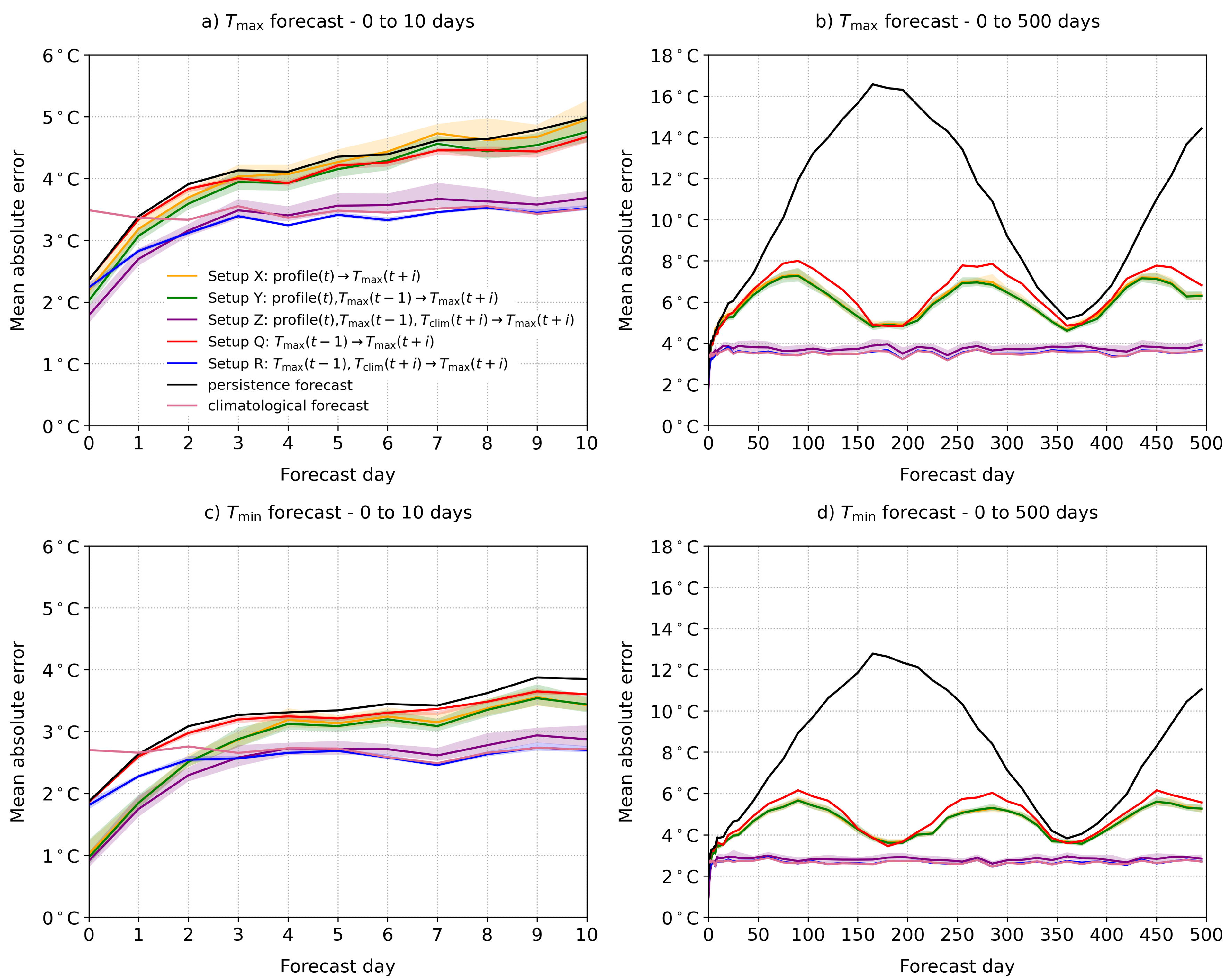
4.2. Forecast Performance

Figure 5 shows the performance of the forecasts at different lead times. The NN forecast of T max based solely on profiles (Setup X, orange line in Figure 5a) barely beats persistence and becomes worse than the climatological forecast already on day two. This is expected, as the radiosonde observation is local and the info it provides is quickly advected downstream throughout the atmosphere. The forecast is slightly improved when the previous-day T max ( t 1 ) is added as an input parameter (Setup Y, green line); however, the best forecast is obtained, when the climatological maximum T clim at the forecast valid time is added as an input variable alongside profiles and previous-day maximum (Setup Z, violet line). The MAE for the present-day forecast is 1.8 °C, thus reduced by 0.5 °C compared to the persistence forecast.
Figure 5c,d show the performance of forecasts of T min . For all lead times, the predictions of T min have a noticeably smaller error compared to predictions of T max . This indicates that the prediction of the minimum temperatures is easier than the prediction of maximum temperatures (e.g., the MAE of climatological forecasts for T min is about 0.8 °C smaller than for T max ). For the same-day forecasts, the prediction is also made easier by the shorter time gap between the early-morning radiosonde observation and time of T min , which typically occurs in the morning. MAE for the present-day forecast of T min is 1 °C for any setup involving measurements of vertical profiles (Setup X, Y, Z). This is approximately 1 °C smaller than the error for T max prediction. The profile-based forecasts beat the persistence forecast at all lead times and become comparable to or worse than the climatological forecast on day three.
Another interesting and unintuitive feature of Figure 5 is that the error is smaller if the extremes are predicted by NN that uses only previous-day extremes (Setup Q, red line) compared to the persistence forecast (black line). This feature is even more evident in the graphs showing the MAE evolution for the long-range prediction of temperature extremes (Figure 5b,d). While such long-range predictions do not have any practical value, they reveal the underlying features of the NN training. For example, the MAE of forecasts using Setups X, Y and Q appears as a sine wave with twice lesser period than the period of persistence MAE. The shape of the latter is obvious, as the MAE is largest at approximately 180 days (forecast issue time and forecast valid time are in exactly opposing seasons) and smallest at roughly 1 year (same seasons). The MAE of forecasts performed with Setups X, Y and Q is largest at 90 days and roughly 270 days, whereas the MAE of persistence forecast is largest at approximately 180 days (half a year). This behavior can be explained by the fact that the NN in Setup X, Y or Q does not know about the current season (or about the season at forecast valid time) and can only indirectly infer this information from available input data (e.g., the temperature profile). The 180-day forecast is thus rather straightforward: if the input temperatures are high (likely summer), then the output temperatures after 180 days will likely be low (winter). Similarly, if the input temperatures are moderate (likely spring or autumn), the output temperatures will remain moderate (likely autumn or spring). However, for the 90-day forecast, the moderate input temperatures (likely spring or autumn) can lead to either high temperatures (likely summer) or low temperatures (likely winter) after 90 days, which results in a larger forecast error.
Taking longer time series of past data as a predictor and using recurrent NNs would likely improve the forecasts, as such NNs are able to grasp the temporal trends. Even a simple predictor such as the day of the year can improve prediction for the long-term forecasts (not shown). The prediction skill could also be enhanced by taking the time of the radiosonde measurement as the predictor. In particular, the minimum temperature prediction is likely sensitive to the time difference between the observation and the occurrence of the daily minimum (typically in the early morning). Another solution is to include the climatological extremes T clim at the forecast valid time t + i as predictors (Setups Z and R). Using such setups, the NN can constrain the long-range forecast MAE to the climatological forecast error (Figure 5). Experimenting with additional options is beyond the scope of this study.

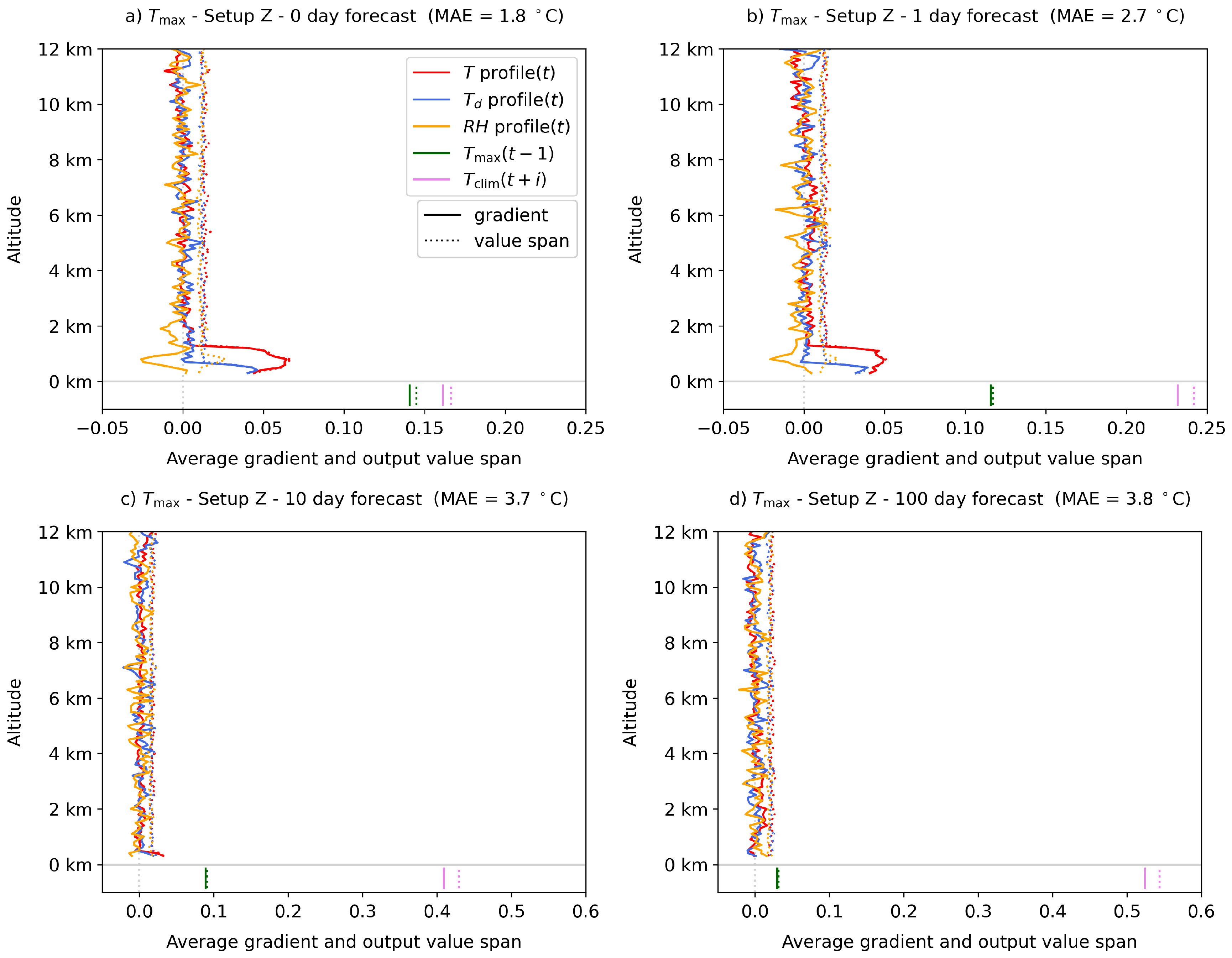
4.3. Network Interpretation

Finally, we explored the impact of our predictors on the forecast. Figure 6 and Figure 7 show results of the XAI analysis for forecasts of T max using Setups X and Z (the results for other setups, some additional forecast lead times and forecasts of T min are shown in the Supplementary Materials in Figures S1–S6). For Setup X, both the average input gradient and the output value span suggest that the medium-range prediction (up to 10 days, Figure 6a–c) is governed mostly by the lowest 1 km of the temperature profile, and the lowest 200 m of the dew-point temperature profile. Low relative humidity in the bottom 1 km is associated with higher temperature extremes. In the first 10 days, the mid- and upper-tropospheric levels barely affect the temperature prediction, as the values of gradient and span are rather small and noisy.
However, the 100-day T max prediction (Figure 6d) is strongly affected by the entire vertical temperature profile, meaning that the network grasps the (seasonal) info on T max from the changing atmospheric profile. First, the larger part of the temperature profile (below 1.5 km and above 5 km altitude) shows a negative impact on T max . If the measured temperatures are low (likely winter), then the forecasted T max will be higher after 100 days (likely spring), and vice versa: high temperatures (likely summer) will lead to lower temperatures after 100 days (likely autumn). Apart from the mean vertical "signal", the neural network also learns the vertical profile of the measured temperatures, which define the T max in 100 days. In the majority of the lower half of the troposphere, the T max exhibits positive sensitivity to measured temperatures, and the opposite in the upper troposphere. This can be explained by the seasonal differences in the average vertical temperature gradient at the location. The average temperature gradient is largest in the summer and smallest in the winter (see Figure S9 in the Supplementary Materials). The larger the vertical temperature gradient (likely summer), the colder the T max in 100 days and vice versa.
It is also worth noting that the spread of the gradient metric is much larger compared to the spread of the value span metric. For example, the typical standard deviation of the gradient values for the setups shown in Figure 6 is about 0.2 for all input variables at all altitudes (see Figure S7 in the Supplementary Materials). This is significantly larger than the average gradient values (which are limited to the range [ 0.1 , 0.1 ] ). Thus, even though the average gradient value might be zero (indicating a rather small overall influence on the forecasted value), the gradient value for a specific day in the test set might be quite large by size and be either positive or negative. In contrast, the standard deviation of the value span metric is much smaller—typically about 0.02 for the setups shown in Figure 6 (see Figure S8 in the Supplementary Materials). Thus it gives a more dependable measure of the influence of a particular predictor on the forecasted value.
Figure 7 show the results of the XAI analysis for forecasts of T max using Setup Z. The two additional predictors ( T max ( t 1 ) and T clim ) have a large influence on the forecasted value. For the same-day forecasts (Figure 7a), both predictors have a comparable influence on the forecasted value, with the importance of the profiles being smaller; however, with longer forecast times the importance of T clim increases, while the importance of T max and the profiles decreases. For the 100-day forecast (Figure 7d) the prediction is almost solely based on T clim . The difference between Figure 6d and Figure 7d is striking, with the profile-based information from the whole troposphere being replaced with a single climatological value, thereby almost halving MAE from 7.1 °C to 3.8 °C. This highlights the adaptability of the NN, which can successfully identify and use the most useful parameters, while the unessential ones are sidelined.

5. Discussion and Conclusions

This study aimed to explore the capability of neural networks that rely on data from radiosonde measurement to predict daily temperature minimums and maximums. More specifically, the aim was to understand how the NN-based models utilize different types of input data and how the network design influences its behavior. The data utilization and behavior of the network depends on whether the NNs are used to do short-term or long-term forecasts—this is why the analysis was performed for a wide range of forecast lead times.
The analysis using very simple NNs, consisting of only a few neurons, highlighted how the nonlinear behavior of the NN increases with the number of neurons. It also showed how different training realizations of the same network could result in different behaviors of the NN. The behavior in the part of the predictor phase space with the highest density of training cases was usually quite similar for all training realizations. In contrast, the behavior elsewhere was more variable and more frequently exhibited unusual nonlinearities. This has consequences for how the network behaves in part of the predictor phase space that is not sufficiently sampled with the training data—for example, in situations that could be considered outliers (such situations can occur but not very frequently). For such events, the NN behavior can be quite different for each training realization. The behavior can also be unusual, indicating that the results for such situations need to be used with caution.
Analysis of selected NN hyperparameters showed that using larger batch sizes reduced training time without causing a significant increase in error; however, this was true only up to a point (in our case up to batch size 256), after which the error did start to increase. We also tested how the number of epochs influences the forecast error and training speed, with 100 epochs being a good compromise choice.
We analyzed various NN setups that were used for the short- and long-term forecasts of temperature extremes. Some setups were more complex and relied on the profile measurements on 118 altitude levels or used additional predictors such as the previous-day measurements and climatological values of extremes. Other setups were much simpler, did not rely on the profiles, and used only the previous day extreme value or climatological extreme value as a predictor. The behavior of the setups was also analyzed via two XAI methods, which help determine which input parameters have a more significant influence on the forecasted value.
For the setup based solely on the profile measurements, the short- to medium-range forecast (0–10 days) mainly relies on the profile data from the lowest layer—mainly on the temperature in the lowest 1 km. For the long-range forecasts (e.g., 100 days), the NN relies on the data from the whole troposphere. As could be expected, the error increases with forecast lead time, but at the same time, it exhibits seasonal periodic behavior for long lead times. The NN forecast beats the persistence forecasts but becomes worse than the climatological forecast already on day two or three (this depends on whether maximum or minimum temperatures are forecasted). It is also important to note the spread of error values of the NN ensemble (which consists of 50 members). The spread of the setups that use the profile data is significantly larger than the spread of the setups that rely only on non-profile data. For the former, the maximum error value in the ensemble was typically about 25% larger than the minimum error value. This again highlights the importance of performing multiple realizations of NN training.
The forecast slightly improves when the previous-day measurements are added as a predictor; however, the best forecast is obtained when the climatological value is added as well. The inclusion of the T clim can improve the short-term forecast—this is interesting and somewhat surprising and shows how the NN models are capable of successfully utilizing the climatological information along the information on the current state atmosphere. Still, the most significant benefit of climatological information is seen for the long-term forecasts where the error is constrained to the climatological forecast error. The analysis by the XAI methods showed that in these cases, the NN prediction is almost solely based on the climatological value and that other predictors have a very small influence. One interesting observation is that, while the average error of the 50-member NN ensemble tends to be larger than the error of the climatological forecast after day three, the ensemble’s minimum error is often a bit smaller. Although the NN ensemble performs worse on average, at least one ensemble member can nevertheless perform a bit better than the climatological forecast. This can happen even for very long-term forecasts (e.g., more than a year into the future). This again highlights the importance of performing multiple realizations of NN traning.
In the end, it is important to point out that although the NN-based prediction systems presented in the study are relatively simple, and cannot be expected to outperform the current state-of-the-art operational NWP models, the analysis nevertheless provides meaningful results, which might have implications for potential future data-driven prediction of the atmospheric evolution from raw observations. For example, the XAI analysis (Figure 6a–c) revealed that the NN is able to diagnose the vertical layers of T, T d and RH that impact the prediction of T m a x the most. This resembles the vertical correlations built into the background-error covariance model for the assimilation of atmospheric observations into NWP models [29]. Analogously as in our case, these vertical correlations act to (objectively) spread the impact of observation across the model domain; however, in analogy to the NWP data assimilation, some localization of the observation impact would be beneficial to reduce the complexity of the network, as the mid- and upper-tropospheric measurements do not contribute anything to the short-range prediction. In the NN context, this can be achieved by dropping out some neurons so that the network only learns the most robust features. The findings derived from the long-range prediction experiments are also relevant for seasonal-to-subseasonal (S2S) climate prediction, where machine learning models have already demonstrated better prediction than the state-of-the-art operational prediction systems [30].

Supplementary Materials

The following are available online at https://www.mdpi.com/article/10.3390/app112210852/s1, Figures S1–S6 show results of the XAI analysis for additional setups, forecast lead times and forecasts of T min , Figures S7–S8 show the spread of the results for the XAI analysis for forecasts of T max by Setup X, Figure S9 shows the average seasonal T profiles.

Author Contributions

Conceptualization, G.S., Ž.Z.; methodology, G.S., D.H., Ž.Z.; software, G.S., D.H., Ž.Z.; formal analysis, G.S., D.H.; investigation, G.S., D.H.; data curation, G.S., D.H.; verification, G.S., D.H.; writing—original draft preparation, G.S., D.H., Ž.Z.; writing—review and editing, G.S., D.H., Ž.Z.; visualization, G.S., D.H.; supervision, G.S., Ž.Z.; project administration, G.S., Ž.Z.; funding acquisition, G.S., Ž.Z. All authors have read and agreed to the published version of the manuscript.

Funding

The authors acknowledge the financial support from the Slovenian Research Agency (Javna Agencija za Raziskovalno Dejavnost RS; research core funding No. P1-0188 and project J1-9431).

Acknowledgments

The authors acknowledge the Slovenian Environmental Agency for willfully sharing the radiosonde-measured and station-measured data.

Conflicts of Interest

The authors declare no conflict of interest. The funders had no role in the design of the study; in the collection, analyses, or interpretation of data; in the writing of the manuscript, or in the decision to publish the results.

References

  1. Reichstein, M.; Camps-Valls, G.; Stevens, B.; Jung, M.; Denzler, J.; Carvalhais, N.; Prabhat. Deep learning and process understanding for data-driven Earth system science. Nature 2019, 566, 195–204. [Google Scholar] [CrossRef] [PubMed]
  2. Palmer, T. A Vision for Numerical Weather Prediction in 2030. arXiv 2020, arXiv:2007.04830. [Google Scholar]
  3. Schultz, M.G.; Betancourt, C.; Gong, B.; Kleinert, F.; Langguth, M.; Leufen, L.H.; Mozaffari, A.; Stadtler, S. Can deep learning beat numerical weather prediction? Philos. Trans. R. Soc. A 2021, 379, 20200097. [Google Scholar] [CrossRef] [PubMed]
  4. Krasnopolsky, V.M.; Fox-Rabinovitz, M.S.; Chalikov, D.V. New Approach to Calculation of Atmospheric Model Physics: Accurate and Fast Neural Network Emulation of Longwave Radiation in a Climate Model. Mon. Weather Rev. 2005, 133, 1370–1383. [Google Scholar] [CrossRef] [Green Version]
  5. Brenowitz, N.D.; Bretherton, C.S. Prognostic Validation of a Neural Network Unified Physics Parameterization. Geophys. Res. Lett. 2018, 45, 6289–6298. [Google Scholar] [CrossRef]
  6. Chantry, M.; Hatfield, S.; Dueben, P.; Polichtchouk, I.; Palmer, T. Machine Learning Emulation of Gravity Wave Drag in Numerical Weather Forecasting. J. Adv. Model. Earth Syst. 2021, 13, e2021MS002477. [Google Scholar] [CrossRef]
  7. Hatfield, S.; Chantry, M.; Dueben, P.; Lopez, P.; Geer, A.; Palmer, T. Building tangent-linear and adjoint models for data assimilation with neural networks. J. Adv. Model. Earth Syst. 2021, e2021MS002521. [Google Scholar] [CrossRef]
  8. Rodrigues, E.R.; Oliveira, I.; Cunha, R.; Netto, M. DeepDownscale: A deep learning strategy for high-resolution weather forecast. In Proceedings of the IEEE 14th International Conference on eScience, e-Science 2018, Amsterdam, The Netherlands, 29 October–1 November 2018; pp. 415–422. [Google Scholar] [CrossRef] [Green Version]
  9. Rasp, S.; Lerch, S. Neural Networks for Postprocessing Ensemble Weather Forecasts. Mon. Weather Rev. 2018, 146, 3885–3900. [Google Scholar] [CrossRef] [Green Version]
  10. Grönquist, P.; Yao, C.; Ben-Nun, T.; Dryden, N.; Dueben, P.; Li, S.; Hoefler, T. Deep learning for post-processing ensemble weather forecasts. Philos. Trans. R. Soc. A 2021, 379. [Google Scholar] [CrossRef]
  11. Chattopadhyay, A.; Hassanzadeh, P.; Pasha, S. A test case for application of convolutional neural networks to spatio-temporal climate data: Re-identifying clustered weather patterns. arXiv 2018, arXiv:1811.04817. [Google Scholar] [CrossRef]
  12. Lagerquist, R.; McGovern, A.; Gagne, D.J., II. Deep Learning for Spatially Explicit Prediction of Synoptic-Scale Fronts. Weather Forecast. 2019, 34, 1137–1160. [Google Scholar] [CrossRef]
  13. Liu, Y.; Racah, E.; Prabhat; Correa, J.; Khosrowshahi, A.; Lavers, D.; Kunkel, K.; Wehner, M.; Collins, W. Application of Deep Convolutional Neural Networks for Detecting Extreme Weather in Climate Datasets. arXiv 2016, arXiv:1605.01156. [Google Scholar]
  14. Weyn, J.A.; Durran, D.R.; Caruana, R. Can Machines Learn to Predict Weather? Using Deep Learning to Predict Gridded 500-hPa Geopotential Height From Historical Weather Data. J. Adv. Model. Earth Syst. 2019, 11, 2680–2693. [Google Scholar] [CrossRef]
  15. Weyn, J.A.; Durran, D.R.; Caruana, R. Improving Data-Driven Global Weather Prediction Using Deep Convolutional Neural Networks on a Cubed Sphere. J. Adv. Model. Earth Syst. 2020, 12, e2020MS002109. [Google Scholar] [CrossRef]
  16. Rasp, S.; Dueben, P.D.; Scher, S.; Weyn, J.A.; Mouatadid, S.; Thuerey, N. WeatherBench: A Benchmark Data Set for Data-Driven Weather Forecasting. J. Adv. Model. Earth Syst. 2020, 12, e2020MS002203. [Google Scholar] [CrossRef]
  17. Rasp, S.; Thuerey, N. Data-Driven Medium-Range Weather Prediction With a Resnet Pretrained on Climate Simulations: A New Model for WeatherBench. J. Adv. Model. Earth Syst. 2021, 13, e2020MS002405. [Google Scholar] [CrossRef]
  18. Scher, S. Toward Data-Driven Weather and Climate Forecasting: Approximating a Simple General Circulation Model With Deep Learning. Geophys. Res. Lett. 2018, 45, 12616–12622. [Google Scholar] [CrossRef] [Green Version]
  19. Jiang, Z.; Jia, Q.S.; Guan, X. Review of wind power forecasting methods: From multi-spatial and temporal perspective. In Proceedings of the Chinese Control Conference, CCC 2017, Dalian, China, 26–28 July 2017; pp. 10576–10583. [Google Scholar] [CrossRef]
  20. Grover, A.; Kapoor, A.; Horvitz, E. A deep hybrid model for weather forecasting. In Proceedings of the ACM SIGKDD International Conference on Knowledge Discovery and Data Mining, Sydney, Australia, 10–13 August 2015; Association for Computing Machinery: New York, NY, USA, 2015; Volume 2015, pp. 379–386. [Google Scholar] [CrossRef]
  21. Ravuri, S.; Lenc, K.; Willson, M.; Kangin, D.; Lam, R.; Mirowski, P.; Fitzsimons, M.; Athanassiadou, M.; Kashem, S.; Madge, S.; et al. Skilful precipitation nowcasting using deep generative models of radar. Nature 2021, 597, 672–677. [Google Scholar] [CrossRef]
  22. Sønderby, C.K.; Espeholt, L.; Heek, J.; Dehghani, M.; Oliver, A.; Salimans, T.; Agrawal, S.; Hickey, J.; Kalchbrenner, N. MetNet: A Neural Weather Model for Precipitation Forecasting. arXiv 2020, arXiv:2003.12140. [Google Scholar]
  23. American Meteorological Society. 2021: Radiosonde. Glossary of Meteorology. Available online: https://glossary.ametsoc.org/wiki/Radiosonde (accessed on 8 November 2021).
  24. Abadi, M.; Barham, P.; Chen, J.; Chen, Z.; Davis, A.; Dean, J.; Devin, M.; Ghemawat, S.; Irving, G.; Isard, M.; et al. TensorFlow: A system for large-scale machine learning. In Proceedings of the 12th USENIX Symposium on Operating Systems Design and Implementation, OSDI 2016, Savannah, GA, USA, 2–4 November 2016; pp. 265–283. [Google Scholar] [CrossRef]
  25. Pedregosa, F.; Varoquaux, G.; Gramfort, A.; Michel, V.; Thirion, B.; Grisel, O.; Blondel, M.; Prettenhofer, P.; Weiss, R.; Dubourg, V.; et al. Scikit-learn: Machine Learning in Python. J. Mach. Learn. Res. 2011, 12, 2825–2830. [Google Scholar]
  26. Wilks, D.S. Statistical Methods in the Atmospheric Sciences; Elsevier: Oxford, UK, 2011; Volume 59, p. 627. [Google Scholar] [CrossRef]
  27. Samek, W.; Müller, K.R. Towards Explainable Artificial Intelligence. In Explainable AI: Interpreting, Explaining and Visualizing Deep Learning; Springer: Cham, Switzerland, 2019; pp. 5–22. [Google Scholar] [CrossRef] [Green Version]
  28. Hechtlinger, Y. Interpretation of Prediction Models Using the Input Gradient. arXiv 2016, arXiv:1611.07634. [Google Scholar]
  29. Bannister, R.N. A review of forecast error covariance statistics in atmospheric variational data assimilation. I: Characteristics and measurements of forecast error covariances. Q. J. R. Meteorol. Soc. 2008, 134, 1951–1970. [Google Scholar] [CrossRef]
  30. Cohen, J.; Coumou, D.; Hwang, J.; Mackey, L.; Orenstein, P.; Totz, S.; Tziperman, E. S2S reboot: An argument for greater inclusion of machine learning in subseasonal to seasonal forecasts. Wiley Interdiscip. Rev. Clim. Chang. 2019, 10, e00567. [Google Scholar] [CrossRef] [Green Version]
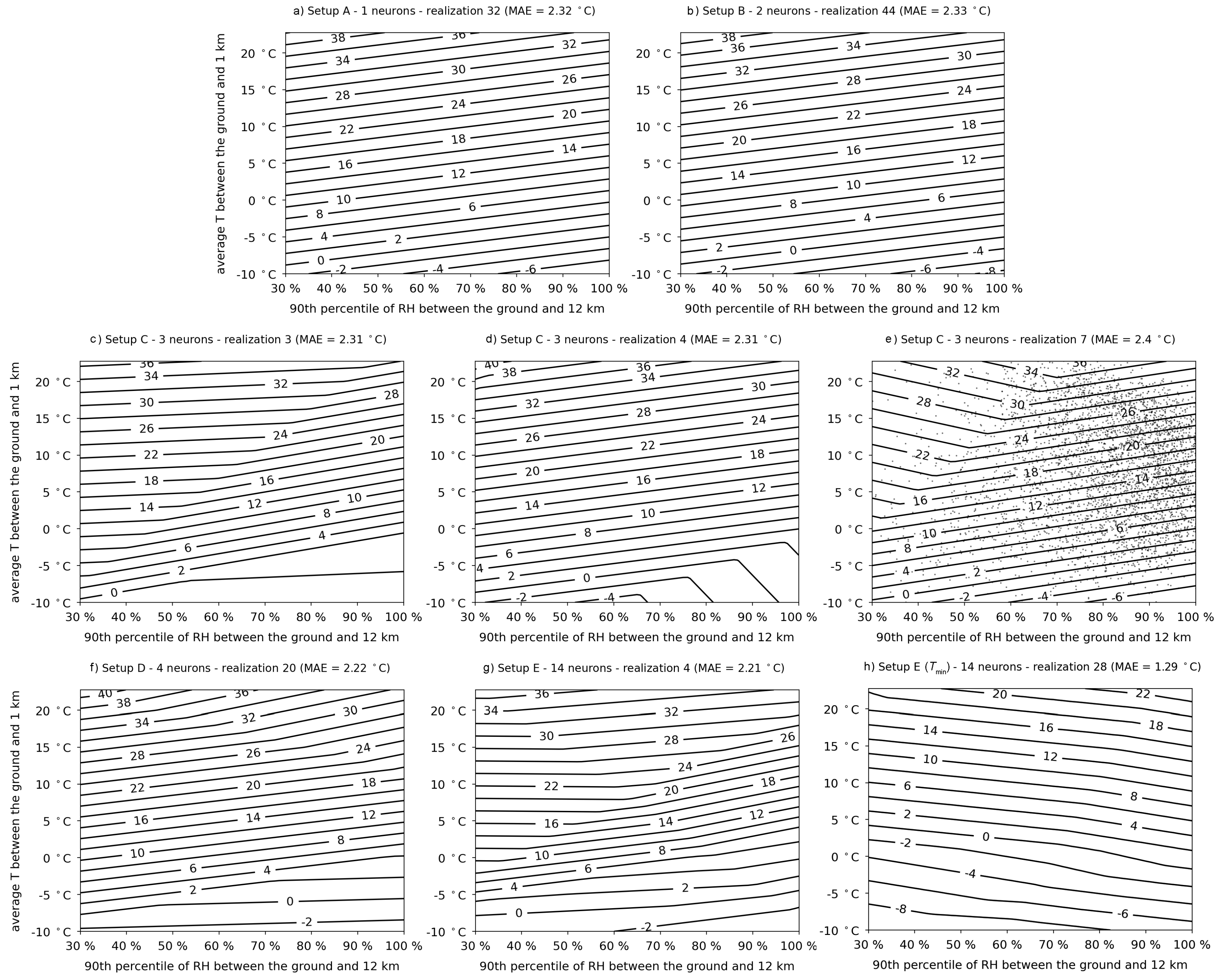
Figure 1. The number of radiosonde measurements in each month that passed the quality control and were used for neural network training, validation and testing; shown with blue bars. Grey bars indicate number of days in each month.
Applsci 11 10852 g001
Figure 2. Correlations of temperature T, dew-point temperature T d and relative humidity R H profiles with (a) T max and (b) T min measured on the same day. The correlations with measurements from the previous-day ( T max ( t 1 ) and T min ( t 1 ) ) and climatological values ( T clim ) are also shown by short vertical lines in the lower part of the graphs.
Applsci 11 10852 g002
Figure 3. An example of training of NN in Setup X (the setup is described in Table 3) for the same-day forecasts of T max ; (a) shows the reduction of the loss function during training while (b) shows the comparison of observed and forecast values of T max in the test set. Red line indicates, where the observed and predicted T max would be equal.
Applsci 11 10852 g003
Figure 4. Analysis of minimalist NNs listed in Table 1. The contours represent the forecasted values of either T max (ag) or T min (h), which depend on two input parameters (the average temperature in the lowest 1 km and the 90th percentile of RH). (e) Also shows the values of the 3800 sets of input parameters that were used for the training, validation and testing of NNs (gray points).
Applsci 11 10852 g004
Figure 5. The evolution of the test set mean absolute error (MAE) for forecast using various NN setups. The setups are described in Table 3. The time index t refers to the day of the radiosonde measurement, with t 1 referring to the previous day, and t + i to the i-th day in the future. The legend is the same for all subfigures as long as T max in (a,b) is replaced with T min in (c,d). For the forecasts made by various NN setups, the lines represent the average MAE values in the ensemble while the color shaded regions indicate the interval between the 10th and 90th percentile.
Applsci 11 10852 g005
Figure 6. The results of the XAI analysis for forecasts of T max by NN Setup X. The subfigures show the analysis for different forecast lead times: (a) 0 day; (b) 1 day; (c) 10 day; (d) 100 day. The average input gradient is shown by solid lines and the average output value span by dotted lines.
Applsci 11 10852 g006
Figure 7. Same as Figure 6 but for forecasts of Setup Z instead of Setup X. The values for input parameters T max ( t 1 ) and T clim ( t + i ) are indicated by short vertical lines in the lower part of the graphs.
Applsci 11 10852 g007
Table 1. Description of the simplistic neural networks consisting of only a few neurons. All setups used the same two input parameters, the average temperature in the lowest layer between the ground and 1 km and the 90th percentile of RH in the layer between the ground and 12 km. The second column denotes the number of neurons in consecutive layers: input layer always contains 2 neurons for 2 input parameters and is not included in the table, whereas the output layer always includes a single neuron. Leaky ReLU was used as activation function for all layers in all setups. The shown MAE values represent the error of the same-day forecast of T max for the testing set. Since 50 realizations of NN training were performed for each setup, the average value, the 10th percentile and the 90th percentile of MAE values are shown.
NameNeurons in LayersMAE avg. [10th perc., 90th perc.]
Setup A12.32 [2.32, 2.33] °C
Setup B1,12.32 [2.29, 2.34] °C
Setup C2,12.31 [2.26, 2.39] °C
Setup D3,12.31 [2.26, 2.38] °C
Setup E5,5,3,12.27 [2.22, 2.31] °C
Table 2. The result of the two XAI methods for the same-day forecast of T max and T min using NN Setup E. The shown values of gradient and value span were averaged over all the test cases and 50 realizations of the training.
T max T min
gradientvalue spangradientvalue span
avg. T in the lowest 1 km1.051.010.970.96
90th percentile of RH−0.160.160.170.18
Table 4. Influence of batch size and number of epochs on the performance of the NN in setup Y. The MAE values are expressed in °C. The execution time represents the time it took to train a single NN on a computer using a Nvidia GeForce RTX 3090 GPU.
Batch Size (Number of Epochs = 100)
124816326412825651210242048
MAE avg.2.032.082.062.052.011.992.022.012.032.062.152.21
MAE 10th perc.1.891.911.901.891.891.881.891.891.931.982.052.09
MAE 90th perc.2.312.422.282.332.112.132.222.142.222.152.312.35
execution time916 s504 s260 s131 s67 s35 s19 s11 s7.3 s5 s3.6 s2.6 s
Number of Epochs (Batch Size = 256)
125101520501001502005001000
MAE avg.8.847.825.543.312.532.342.112.011.991.981.971.99
MAE 10th perc.7.306.593.252.362.162.101.991.911.901.871.881.90
MAE 90th perc.10.008.917.366.052.912.652.282.222.142.172.112.07
execution time0.4 s0.5 s0.7 s1.0 s1.4 s1.7 s3.8 s7.3 s11 s14 s35 s70 s
Publisher’s Note: MDPI stays neutral with regard to jurisdictional claims in published maps and institutional affiliations.

