A Novel Tradeoff Analysis between Traffic Congestion and Packing Density of Interconnection Networks for Massively Parallel Computers

Abstract

From disaster prevention to mitigation, drug analysis to drug design, agriculture to food security, IoT to AI, and big data analysis to knowledge or sentiment mining, a high computation power is a prime necessity at present. As such, massively parallel computer (MPC) systems comprising a large number of nodes are gaining popularity. To interconnect these huge numbers of nodes efficiently, hierarchical interconnection networks are an attractive and feasible option. A Tori-connected flattened butterfly network (TFBN) has been proposed by the authors in a prior work for future generation MPC systems. In the previous study, the static network performance and static cost-effectiveness were evaluated. In this research, a novel trade-off factor named message traffic congestion vs. packing density trade-off factor has been proposed, which characterizes the message congestion in the network and its packing density. The factor is used to statically assess the suitability of the implementation of an interconnection network. The message traffic density, packing density, and new factor have been evaluated for the proposed network and similar competitive networks such as TTN, TESH, 2D-Mesh, 3D-Mesh, 2D-Torus, and 3D-Torus. It has been found that the performance of the TFBN is superior to the other networks.

1. Introduction

The unprecedented advancements in modern technology have caused the fields of electricity, electronics, and computer systems to merge in such a way that they are no longer disjointed sets. Particularly, to make electric power systems more automated, secure, and resilient, the application of machine learning, artificial intelligence, big data, and deep learning in the modern utility grids and smart grids is accelerating at an exponential rate [1,2]. As such, the importance of a high computational power is undeniable to ensure that the widely encompassing systems are operating as desired.

Due to its high computational power, massively parallel computation (MPC) is required in all aspects of modern life, including disaster prevention and mitigation, healthcare, drug design, personalized medicine, etc. Moreover, due to the enormous shift of professional activities into a full virtual mode at the onset of the COVID-19 pandemic, the world has truly realized the importance of fast computation at a low power consumption. Computational speeds as high as exa-flops or even zetta-flops are not only good-to-have in the next-generation supercomputers for MPCs, but rather a must-have criterion in order to keep marching forward in the computer network industry [3,4,5,6].

Although low dimensional networks are better in terms of their lesser delay and higher throughputs [7,8], they are not suitable for interconnecting millions of nodes for a hierarchical interconnection network (HIN) [9,10,11]. For next-generation systems of MPC, the interconnection of more than a million nodes, a combination of low-dimensional networks and the topology is required [12]. HINs have been adequately described in the literature as a revolutionary milestone for massively parallel computers and nest-generation parallel computing. For instance, the extended hypercube [13], Tori-connected mesh (TESH) [14], hierarchical torus network (HTN) [15], rectangular twisted torus meshes (RTTM) [16], midimew connected mesh network (MMN) [17,18], hierarchical Tori connected mesh network (HTM) [19], shifted completely connected network (SCCN) [20], 3-dimensional Tori connected torus network (3D-TTN) [21], and many more networks have been proposed and assessed in recent years as a means to promote MPC systems. The numerous works pertinent to the HIN is testament to its numerous benefits in terms of network performance and computational speed. The prime advantage of HIN lies in the reduced link cost and the inherent coordination and communication among the many nodes within the network [22].

The concept of a novel HIN named Tori-connected flattened butterfly network (TFBN) had been posited by the authors in an earlier work [23] along with a statistical analysis of its performance. The network contains several interconnected basic modules (BMs) for forming the networks that indicate higher level in the hierarchy. The BMs are actually a 2D flattened butterfly network [24] and each higher level is a 2D torus network; hence the name of the new network. The specialty of the TFBN is that it reduces network congestion and augments the throughput in the BMs.

Although the very first study on the proposed TFBN shows good static network performance compared to other networks, further investigation is substantial to establish TFBN as a reliable HIN topology. Since the practical implementation is quite expensive, a static evaluation and then experimentation by simulation is a better alternative to assess the superiority of any network. In this research, we explore the density parameters of the network statically. The main objectives of this paper are to statically assess the packing density, message traffic density, and a new parameter called traffic congestion versus packing density trade-off factor (TCPDTF) to show the eminence of the proposed TFBN.

The rudimentary study on the packing density of TFBN is presented earlier, and only the packing density of a Level-2 TFBN with only 256 nodes is presented in that article [25]. In another addition, it has been proven that the TFBN has a low hop distance, which is an attractive feature of a HIN [26]. However, the detailed study on density parameters along with their trade-off analysis of the proposed TFBN has not been carried out yet. Therefore, the aim of this study is to assess the static performance of the TFBN in comparison with other networks by determining the static network performance parameters for the higher-levels of the TFBN network, density parameter analysis, and the trade-off between these density parameters.

The remaining part of the paper is arranged as follows. Section 2 and Section 3 describe the architecture of the TFBN network and the routing mechanism within the network, respectively. Section 4 analyzes the static network performance of the TFBN for both lower and higher levels. Next, the density parameters and their trade-off factor are analyzed in Section 5, along with the presentation of the novel parameter. Then, Section 6 delineates the main outcomes of this work and also provides the future research directions based on the outcome. Finally, the conclusion of this framework is disclosed in Section 7.

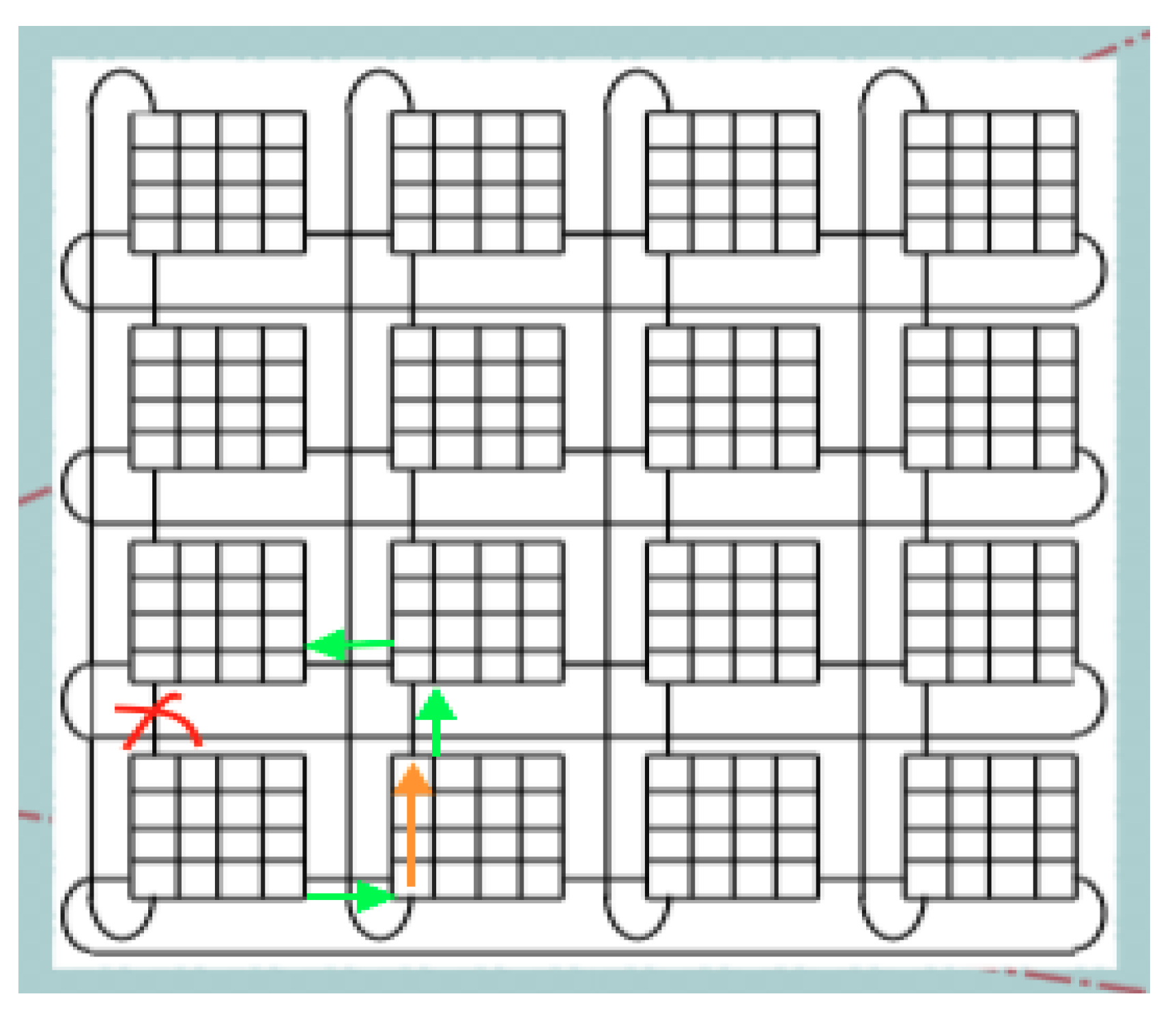
2. Interconnection of the TFBN

The proposed TFBN network comprises of multiple basic modules (BM) in a hierarchical arrangement. This section describes the BM of the TFBN first, and follows with the description of the overall higher level network.

2.1. Basic Module of the TFBN

The BM of the TFBN is a flattened butterfly network as a $(2^m\times 2^m)$ 2D-Torus network with $2^{2m}$ nodes. For networks with a high node degree, the flattened butterfly architecture is highly cost-efficient [24]. Each of the nodes is characterized by $2^m$ rows and $2^m$ columns, where m is a positive integer. The value of m is preferred to be 2 due to a higher value of granularity of the network. So, the size of the BM is $(4\times 4)$ as illustrated in Figure 1. Each BM has $2^{(m+2)}$ free ports for establishing higher-level networks. This is the Level-1 network of the TFBN.

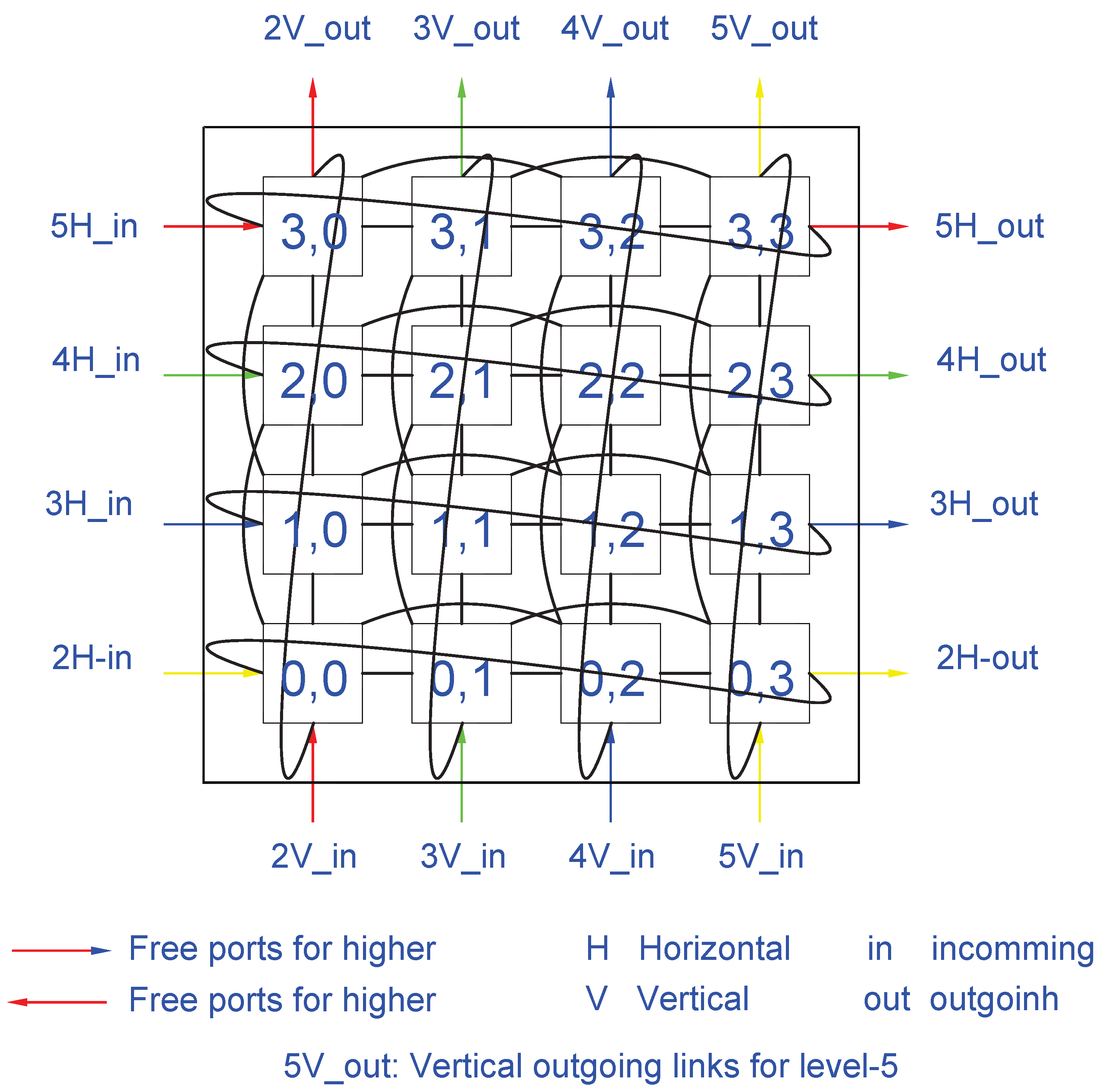
2.2. Higher Level Networks of the TFBN

Connecting $2^{2m}$ lower networks with a 2D-Torus network in $2^m$ rows and $2^m$ columns analogous to the BM, the higher levels of the TFBN are initiated. Thus, with $(m=2)$, 16 Level-1 networks can be connected to form Level-2, and 16 Level-2 networks can be connected to form Level-3, and so forth. Figure 2 depicts the lay out of the higher-level networks of TFBN. q is the inter-level connectivity. In each BM, $4\times 2^q=2^{(q+2)}$ free wires and their corresponding ports are used for the higher-level connections. The $2\left(2^q\right)$ links are used for both vertical and horizontal connections, where $q\in 0,1,\dots ,m$ is the inter-level connectivity. Figure 2 shows a $(4\times 4)$ BM with $2^{(2+2)}=16$ free ports, with $m=2$. If $q=0$, there are four free ports for each higher level—two for horizontal and two for vertical interconnections. Bidirectional links are formed by tying incoming and outgoing links (both vertical and horizontal) to connect two adjoining BMs of the higher levels of TFBN.

The value of m, the inter-level connectivity (q), and the level of hierarchy (L), determine the size of the BM, which is denoted by $(m,L,q)$. For higher granularity, $m=2$ has been taken. The highest hierarchical level that can be generated from a $(2^m\times 2^m)$ BM is $L_{max}=2^{(m-q)}+1$.

For example, if $m=2$ and $q=0$, then $L_{max}=2^{(2-0)}+1=5$. Thus, Level-5 is the highest level obtainable in a TFBN with $(4\times 4)$ BMs connected hierarchically. In each level, the number of nodes is $N=2^{2mL}$. So, for the 5-level TFBN considered here, the number of nodes is $N=2^{2m(2^{(m-q)}+1)}=2^{20}=$ 1,048,576. Thus, more than a million nodes can be connected in a 5-level TFBN for an MPC system.

3. Routing Algorithm for TFBN

The process of delivering and receiving messages between two systems is described by a routing algorithm. To shift from a source node to a destination node, it streamlines the designation of path by using a message incorporated in the network. The execution of the interconnection network, which is a critical component in the MPC system, is heavily influenced by message routing expertise and outline of the router. To route a message from the source to its objective in a TFBN, the routing method is divided into three parts [27].

• Phase I: The message in the source BM is directed to a suitable gate node for routing to the higher level network.
• Phase II: The message is directed through the higher level network. The routing procedure is reversed after reaching the highest level, and the message is routed to a gate node in the destination network.
• Phase III: The message is sent from the destination BM’s gate node to the target node within the BM.

The routing mechanism is the same, but the reverse in Phase I and Phase III. The only difference is that Phase I occurs in the source BM while Phase III occurs in the destination BM. When the packet is created in the source node, the destination is verified. In case of being the source and the destination nodes in separate BMs, all the three phases will be applicable. If the source and destination nodes are in the same BM; however, the routing mechanism will only work within that BM. IOnly Phase 1 will be used in this case. A standard preordained dimension-order routing protocol is used to make the routing procedure easier, with the message being sent vertically first and then horizontally.

4. Static Network Performance of a TFBN

The proposed TFBN’s static network performance was evaluated previously, and its superiority over other networks was established in our initial study on TFBN [23]. This paper investigates and analyses the density parameters called message traffic density and packing density, and the trade-off between them. For the analysis, two hop distance parameters (average distance and diameter) and two cost parameters (node degree and wiring complexity) are evaluated for the TFBN. Next, the fault diameter is investigated. This section explains the hop distance parameters, the cost parameters, the fault tolerance, and the fault diameter for the TFBN.

4.1. Hop Distance Parameters

The hop distance is the distance between two directly linked nodes, and it is an essential metric to consider while evaluating the production of any interconnection network architecture in its graph-theoretic model. All distinct sets of nodes in a network contains the highest and the average hop distance using the shortest-path algorithm are termed as diameter and average distance, respectively. These two static network performance parameters are crucial for any interconnection network because they help to understand the possible effect on traffic congestion (message traffic density) as well as predicting the dynamic performance (nature of throughput vs. latency). The diameter is the latency’s upper bound, i.e., the latency at saturation throughput. The average distance, on the other hand, is the latency at no load and no network throughput. A lower value of the hop distance is preferred, as it enhances the dynamic performance communication of the network. Different interconnection networks tend to perform differently on distinct traffic patterns and their respective traffic density. Especially, it is crucial to estimate the zero traffic load latency and possible increase in latency for high traffic load.

The hop distance parameters were simulated using a dimension order routing algorithm. Both diameter and average distance have been enlisted in

Table 1. A comparison of the static network performance of various networks.

Network	Node Degree	Wiring Connectivity	Diameter	Average Distance	Static Cost	Fault Diameter
256 Node
2D-Mesh	4	480	30	10.67	120	32
2D-Torus	4	512	16	8	64	18
TESH	4	416	21	10.47	84	24
TTN	6	544	15	7.44	90	18
TFBN	8	800	10	5.75	80	14
4096 Node
2D-Mesh	4	8064	126	42.67	504	128
2D-Torus	4	8192	64	32.00	256	66
3D-Mesh	6	11,520	45	16.00	270	47
3D-Torus	6	12,288	24	12.00	144	26
TESH	4	6680	32	17.80	128	35
TTN	6	8736	24	12.60	144	27
TFBN	8	12,832	19	10.61	152	23

, which shows that the hop distance parameters of the proposed TFBN [23] outperforms the 2D and 3D mesh and torus networks and hierarchical TTN and TESH network for 256 nodes as well as for 4096 nodes. Furthermore, as the number of nodes increases, the diameter and average distance of hierarchical networks improve significantly than conventional mesh and torus networks. Among them, TFBN yields substantially low hop distance parameters compared to TTN and TESH networks.

4.2. Cost Parameters

An MPC system connects its numerous nodes using connecting wires and so, a huge number of wires is required. A node consists of core, node-level shared memory, and the neighboring nodes are tied together using connecting wires through the router. For example, the fastest computer Fugaku [28] has a computing power 442 petaflops, and it consumes 29,899 kW of electric power. The other supercomputer named Quriosity with a computing power of 1.75 petaflops, ranked in the Top500 [28] supercomputers, and requires a total length of 15 km of wiring and consumes roughly 600 kW of electric power.

4.2.1. Node Degree

The maximum number of links required to connect all surrounding nodes is called the degree of a node. Modern MPC systems have wiring between nodes. As they require large amounts of wiring, it is necessary to keep wiring to a minimum to save costs. Network topology has a pre-defined constant degree, and the higher it is, the higher the cost of a single node is, as the network requires much more connecting wires and static power. Further, considering the required scalability of MPC systems, it would be ideal to have a constant degree of a node because a variable degree will increase the complexity of network scalability, which is costly. Hierarchical networks are specially designed to support the present configuration of MPC system; many research analyses show that hierarchical interconnection network is more preferable than the flat or conventional networks such as torus and mesh.

It is outlined in Table 1 that the degree of a node of the TFBN is constant at 8, which is higher than that of TESH, mesh, torus, and TTN networks. The high node degree will produce the message traffic congestion vs. packing density trade-off factor (TCPDTF) of the proposed hierarchical interconnection network TFBN as portrayed in Section 5.

4.2.2. Wiring Complexity

In an interconnection network, the wiring complexity implies the combination of all the interconnected links in the network. The cost of the entire system rises with the increase in wiring complexity. The TFBN consists of numerous BMs in the form of a 2D-Torus network. The wrap links in these BMs result in a large number of communication links, which incur high level of wiring complexity. The wiring complexity of a TFBN is given by Equation (1), where L is the level number and q is the inter-level connectivity.

$$Wiringcomplexity=\#\mathrm{of}\mathrm{links}\mathrm{in}\mathrm{a}\mathrm{BM}\times k^{2(L-1)}+\sum _{q=2}^{L}2\left(2^q\right)\times k^{2(L-1)}.$$

(1)

The wire complexity of the TFBN is larger than that of torus, mesh, TESH, and TTN networks, as seen in Table 1. The BM has a smaller diameter and average distance due to the extra-short length wrap-around links.

4.2.3. Static Cost

The node degree multiplied by the diameter equals the static cost (Equation (2)). Similar to the hop distance, a low static cost is preferable for any interconnection network. Table 1 summarizes the static cost analysis for TFBN. The table shows that a 2D-Mesh requires the highest static cost and TFBN network requires the lowest static cost with 256 nodes. However, with 4096 nodes, 2D-Mesh fails to improve its previous position, and TESH leads the static performance due to its low node degree (4) compared to TFBN with a node degree of eight.

$$Staticcost=Nodedegree\times Diameter.$$

(2)

The cost parameters and hop distance parameters of the TFBN had been reported in the earlier work. However, we need these parameters again for the evaluation and analysis of the trade-off between traffic congestion and packing density of interconnection networks for an MPC system. Table 1 demonstrates that both the node degree and wiring complexity of the TFBN is high, which yielded quite low values of the hop distance parameters in comparison with other networks considered in this study.

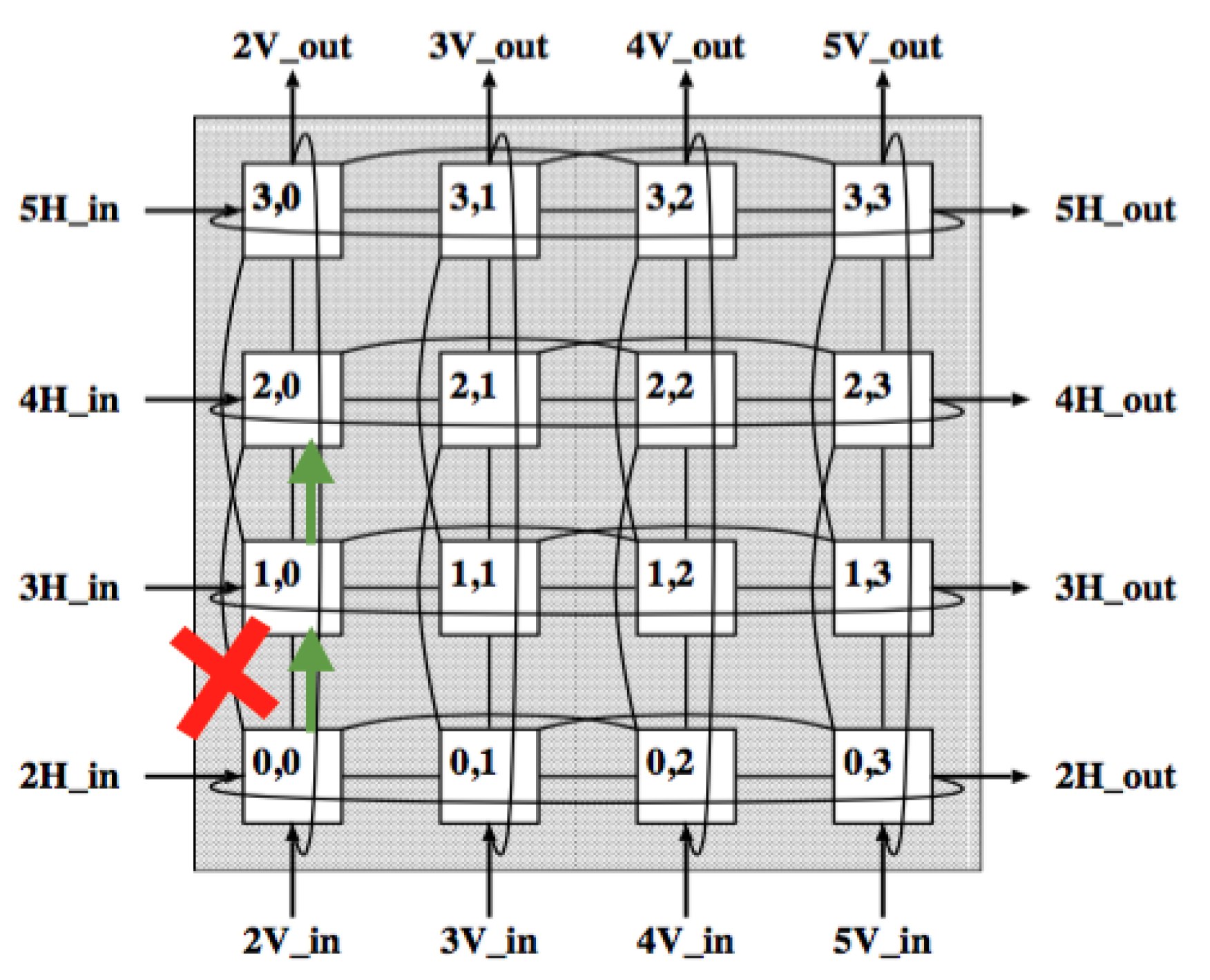
4.3. Fault Tolerance

Fault tolerance is a common and important parameter that must be analyzed during the design phase of interconnection networks. The fault tolerance is determined by the connectivity of the graph, where fault tolerance is the highest possible number of vertices that can be disconnected from the graph before the node becomes fully disconnected from the network i.e., the node becomes completely unreachable. High fault tolerance for any network is always desirable; however, it results in a high node degree of the network, which eventually increases the power usage for the node–node packet routing. The $4\times 4$ BM of TFBN network can support up to five links, which means a $4\times 4$ BM of TFBN has a connectivity of six. On the other hand, a TFBN(2, L, 0) with $m=2$ can still be connected to up to six links.

4.4. Fault Diameter

Unlike the fault tolerance, the fault diameter helps to determine the communication delay and also to track the changes in network diameter if there are f faulty vertices (with f fault tolerance). Moreover, diameter estimation on networks is important if there is a faulty node or a link failure on the network.

Theorem 1.

The fault diameter of TFBN is its network diameter + 4.

Proof of Theorem 1.

TFBN(2, L, 0) has BM connectivity and at most two-higher level connectivity. So, the fault tolerance of TFBN(2, 1, 0) is five and TFBN(2, L, 0) is six. Now, if we consider a scenario that there is a faulty node(1, 0) exits in a TFBN(2, 1, 0) and we would like to transmit the packet from node(0, 0) to node(2, 2). Then, node(0, 0) can directly send packet to node(2, 0) and after that to node(2, 2) even if we follow the YX-order routing. On the other hand, let us consider the Figure 3, if there is a link failure between the node(0, 0) to node(2, 0) then the packet needs to be transmitted through node(1, 0). Hence, fault diameter for basic module of TFBN requires network diameter + 1. The higher level network of TFBN considers 2D-Torus network for its BM to BM connectivity. The Level-2 network of TFBN consists of 16 BMs and the Level-3 network consists of $16\times 16=256$ BMs. Suppose a link failure occurs from BM(0, 0) to BM(1, 0) at Level-2 as shown in Figure 4. For transmitting the packet from BM(0, 0) to BM(1, 0) and considering the routing of XY-order (considering minimum hop distance), packets need to be transmitted to BM(0, 1) and then BM(1, 1) and finally, they will reach BM(1, 0), which results in a fault diameter equal to network diameter + 4. □

Table 1 shows the fault diameter for different networks. For 256 nodes, a 2D-Mesh network requires a network diameter of 30 and a fault diameter of 30 + 2 = 32. In case of 4096 nodes, the same network requires diameter of 126 and fault diameter of 128. Now, since the diameter of TFBN is 10, the fault diameter is 14 and it is less than the fault diameter of TTN (18), TESH (24), and 2D-Torus (18) with 256 nodes. Again, considering 4096 nodes, the fault diameter of TFBN is 23, which is also less than TTN (27), TESH (35), and 3D-Torus (26) networks.

The question may emerge why we have taken Level-2 (256 nodes) and Level-3 (4096 nodes) for performance analysis. The performance is evaluated using the shortest path algorithm with the help of dimension order routing for all distinct pairs of nodes. If the number of the nodes increase, the number of pairs is also exponentially increased, which in turn takes huge time for evaluation. Since TFBN is a hierarchical interconnection network, it will yield better performance with the increase in hierarchy level as we have seen scaling up from Level-2 to Level-3, as depicted in Table 1. We have also observed the improvement of performance with the increase in hierarchy level for the TTN as presented in Ref. [29].

5. Analysis of Trade-Off between Traffic Congestion and Packing Density

The practical implementation of an MPC system is highly expensive. For instance, the manufacturing of the fastest computer Fugaku [28] cost billions of dollars; therefore, before going to practical implementation, any interconnection network topology must be assessed in different stages with respect to different parameters. We explored the primary agenda of this article in this section, i.e., the analysis of the trade-off between traffic congestion and packing density. Two parameters have been analyzed for the static density parameter trade-off analysis—packing density and message traffic density.

5.1. Packing Density

The actual packing density of an HIN depends on five main factors, such as:

1.

How the MPC system is practically implemented from chip level to the system level.

2.

Number of cores interconnected at the chip level to form a node.

3.

Number of nodes interconnected at the board level to form the BM.

4.

Number of BMs interconnected to form the intermediate level network at the cabinet level.

5.

Number of cabinets interconnected to form an MPC system.

Each level has different kinds of links used for the interconnection, ranging from VLSI links at the chip level to optical fiber links at the system level. So, interconnecting such a huge number of cores, nodes, BMs, and cabinets involve numerous communication links and different levels of wiring complexity at each level. The packing density helps to assess the density of the interconnected nodes at each level, and is expressed as the number of nodes per unit cost of an MPC system (Equation (3)).

$$\begin{array}{c}\hfill PackingDen.=\frac{\#Nodes}{StaticCost}=\frac{\#Nodes}{Degree\times Diameter}\end{array}$$

(3)

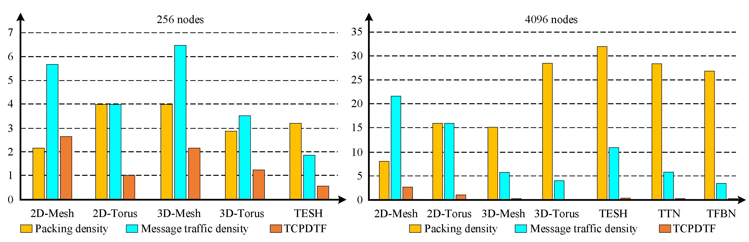
Considering the node degree and diameter of different networks, the packing density of the interconnection networks have been calculated according to the derived Equation (3) and then enlisted in

Table 2. Performance comparison of the packing density, message traffic density, and the TCPDTF of various networks.

Network	Packing Density	Message Traffic Density	Traffic Congestion vs. Packing Density Trade-off Factor (TCPDTF)
256 Nodes
2D-Mesh	2.13	5.69	2.668
2D-Torus	4.00	4.00	1.00
%hline TESH	3.05	6.44	2.114
TTN	2.84	3.50	1.231
TFBN	3.20	1.84	0.575
4096 Nodes
2D-Mesh	8.13	21.67	2.667
2D-Torus	16.00	16.00	1.00
3D-Mesh	15.17	5.69	0.375
3D-Torus	28.44	4.00	0.141
TESH	32.00	10.91	0.341
TTN	28.40	5.91	0.208
TFBN	26.90	3.39	0.125

. For the Level-2 network, it is found that the TFBN has a greater packing density than the TESH, 2D-Mesh, and TTN networks. In fact, it is also higher than 2D-Torus, 2D-Mesh, and 3D-Mesh networks and comparable with TESH, 3D-Torus, and TTN networks in the case of the Level-3 network. However, for the Level-3 TFBN, the packing density is lower compared to 3D-Torus, TESH, and TTN networks because the node degree of the TFBN is substantially higher than the other networks, whereby the number of nodes is the same for all the networks. Even with the high node degree, the TFBN yields similar packing density to those of 3D-Torus, and TESH, and TTN because of its low diameter.

5.2. Message Traffic Density

The main idea underlying the parallel computer systems is to distribute the computation work to many nodes. After that, the outcome of the individual node’s results are merged together to have the final result of the problem or task to be solved. Initially the traffic is a bit less, however, it will be congested as more and more packets are injected in the network. The phenomena resembles traffic congestion on city road network.

Usually the traffic density of packets in a network absolutely depends upon the computation problem being executed in an MPC system or the traffic patterns created for that computation problem. The message latency and network throughput are dependent on the traffic situation or traffic congestion in the network and the deploying routing algorithm. The evaluation of these two parameters by computer simulations or prototype design is quite challenging, tiring, and also quite expensive; therefore, before going to the evaluation of latency and throughput, it is necessary to statically justify whether or not the network will result low latency and high throughput. This statistical assessment can be carried out by evaluating the message traffic density (MTD), or the packet distribution in a network.

The number of links in each node denotes the average number of pathways to transfer a message from one node to another. The average distance is calculated as the mean of the distances between each distinct pair of nodes using the shortest path algorithm. The average distance as well as the total number of nodes and links in an MPC system should be known in order to calculate the MTD. The MTD is calculated by multiplying the average distance by the ratio of total nodes to total connections, which produces the efficiency of traffic distribution in a network, as shown in Equation (4).

$$\begin{array}{c}\hfill MTD=AverageDistance\times \frac{\#ofNodes}{\#ofLinks}\end{array}$$

(4)

The message traffic density of the studied interconnection networks have been calculated according to the derived Equation (4) and then enlisted in Table 2. The results portray that TFBN is much less congested compared to all the other studied networks because the MTD of the TFBN is much lower than all 2D networks such as torus, mesh, TESH, and TTN networks and even remarkably lower than 3D-Torus and 3D-Mesh networks for both 256 and 4096 nodes.

5.3. Trade-Off between Traffic Congestion and Packing Density

The main contribution of this work is the statistical analysis of the density parameters, especially the trade-off between packing density and MTD. The packing density reveals the number of nodes per unit static cost, without considering the number of communication links in the packaging. On the other hand, in an MPC system, messages passes via communication links among all the nodes. So, more links mean more ways for a message to arrive at its intended destination. Moreover, the results from individual nodes can be merged to obtain the final results of computational intensive problems. This alternative path gives alternative choices in a routing algorithm to send the message to its destination. The number of links grows as well with an increment of node number.

After manufacturing an MPC system, the nodes and their associated communication links become fixed and cannot be altered. Only the board level and system level nodes can be altered; however, the efficient use of communication links will lessen the MTD; therefore, after realization of a MPC system, the distribution and coordination of the packets among the nodes by the efficient use of communication links reveal the success of a MPC system. Since evaluation of traffic congestion effect on packing density after practical realization of a MPC system is quite expensive, the static trade-off analysis between traffic congestion and packing density is important to assess if the interconnection network will be suitable or not for the future generation MPC system.

The trade-off factor between message congestion and packing density, called TCPDTF, is defined as the ratio between MTD and packing density. It is represented as in Equation (5), as the product of the average distance and static cost per communication link.

$$\begin{array}{ccc}\hfill TCPDTF& =& \frac{MessageTrafficDensity}{PackingDensity}\hfill \\ & =& \left\{\frac{Avg.Dist.\times \#ofNodes}{\#ofLinks}\right\}\times \left\{\frac{StaticCost}{\#ofNodes}\right\}\hfill \\ & =& \left\{\frac{Avg.Dist.\times StaticCost}{\#ofLinks}\right\}\hfill \end{array}$$

(5)

The traffic congestion and packing density trade-off factor (TCPDTF) of various networks were calculated according to Equation (5) and then enlisted in Table 2. For 256 node networks, the TCPDTF of the proposed TFBN is much lower than 2D- and 3D-Torus, as well as 2D- and 3D-Mesh networks. For 4096 node networks, the TCPDTF of the proposed TFBN is also lower than both 2D- and 3D-Mesh, 2D- and 3D-Torus, and TESH and TTN networks. The portrayed results also reveal that the proposed TFBN has less traffic congestion compared to the other networks. For the TFBN, less traffic congestion means lower latency and higher throughput. These insights can also be observed from the graphical representation of Table 2 in Figure 5. The graph shows the performance comparison for both 256 nodes and 4096 nodes.

6. Outcome of the Study and Future Works

For assessing the performance of computer networks, a novel parameter has been proposed in this paper. The parameter has been named the traffic congestion and packing density trade-off (TCPDTF) factor. The derivation, usage, and significance of this factor has been elaborated in this work. In addition, the performance of the TFBN proposed in an earlier work has been thoroughly analyzed in this study in comparison with the existing networks for HIN. The evaluated results of the several parameters has justifies that TFBN possesses several attractive features. To summarize, the TFBN can be characterized with the following features:

• Low hop distance—The node diameter and the average distance are short in a TFBN.
• High wiring complexity—The BM of a TFBN consists of a flattened butterfly network, which needs many short length links, resulting in a high wiring complexity compared to other networks.
• High node degree–Using the extra links for the BM interconnections increases the node degree of the TFBN.
• High static costs—The TFBN’s static cost is slightly higher than the TTN and TESH networks due to its high node degree, although the cost is substantially less expensive than the torus and mesh networks. So, TFBN can be an ideal candidate as a HIN topology for an MPC system with zetta-scale or exa-scale computation speeds.
• Low traffic congestion—TFBN yields lower traffic congestion with respect to the 3D-Torus network, which is practically implemented in industries for a lot of contemporary MPC systems.
• High packing density—The packing density of TFBN is higher than that of torus and mesh networks and almost similar to that of TTN and TESH networks.
• Low message traffic density—The MTD of the TFBN is far lower than that of both 2D and 3D-Torus and mesh, TESH, and TTN networks.
• Low TCPDTF—The TCPDTF of TFBN is quite lower than that of both 2D- and 3D-Mesh, TESH, 2D-Torus, and TTN networks. It is also considerably lower than that of 3D-Torus networks.
• Low latency—The TFBN has a low latency, i.e., round trip delay, due to the low hop distance parameters–average distance and diameter.
• High throughput—Because of the low hop distance parameters, the TFBN has a high throughput.

The low hop distance, low message traffic density, and low TCPDTF indicate that the TFBN can yield good dynamic communication performance; however, apart from this study, there is still a chance of proceeding the related research work in terms of industry adoption of TFBN for the development of a new MPC system.

6.1. Some Generalization

In this paper a new static parameter called traffic congestion and packing density trade-off factor (TCPDTF) is proposed to assess the interconnection networks. Along with this, we have also evaluated the packing density, message traffic density, and fault diameter. The lower the value of TDPDTF indicates better dynamic communication performance (low latency and high throughput). Before the dynamic communication performance simulation, if a single static parameter indicates its nature, then it is wise to assess the interconnection networks using that unique parameter.

6.2. Future Works

For a thorough evaluation of network performance, the two metrics (latency and throughput) must be evaluated using deterministic dimension order routing and adaptive routing algorithms [30,31]. Statically, the TFBN is less traffic congestive with a high packing density; however, an implementation of prototype by FPGA is necessary for the TFBN cost analysis [32].

7. Conclusions

Studying the performance of computer networks is a zeitgeist in the virtual world created by the COVID-19 pandemic. In such trying times, the necessity of hierarchical interconnection networks for massively parallel computing has be reinstated for high-speed computational networks, such as the TFBN. This article has revolved around the assessment of the density parameters, viz. message traffic density and packing density, to demonstrate the superiority of the proposed TFBN in comparison with the other popular network topologies such as 2D- and 3D-Mesh and torus networks, and hierarchical TTN and TESH networks. The TFBN’s architectural structure has been thoroughly explored and its performance is evaluated using the density parameters. In addition, a new factor has been proposed in this work; it has been named traffic congestion versus packing density trade-off factor (TCPDTF). The factor has been used to assess all the interconnection networks to compare their performance. The cost parameters and hop distance parameters have also been evaluated for all the networks to calculate the density parameters and the TCPDTF. It has been found that among all the networks studied, the performance of the TFBN notably excels in terms of the static network parameters.