Holistic Impact and Environmental Efficiency of Retrofitting Interventions on Buildings in the Mediterranean Area: A Directional Distance Function Approach

Abstract

The study focuses on the application of a nonparametric methodology for evaluating the sustainability of retrofitting interventions to be applied on different typologies of buildings and different climate zones of the Mediterranean area. The paper starts from the analysis of data collected through the HAPPEN project, that is a H2020 European project which proposes a holistic approach for a deep and sustainable renovation of the Mediterranean residential Building stock. Even if the European Commission allocated considerable funds for retrofitting interventions, the choice of the optimal solution is not always that easy because several variables have to be considered. The present manuscript proposes a methodology to compare different retrofitting solutions combining Life-Cycle Cost (i.e., LCC) estimations with the nonparametric Directional Distance Function approach (i.e., DDF). In detail, the literature suggests that the DDF can be effectively used for comparing different observations through efficiency scores. The main result of the paper is the definition of a hybrid methodology that, starting from estimates of LCC and applying a DDF technique, represents a simple method for evaluating the best retrofitting intervention. Results are represented by two scores where the former represents a holistic efficiency measure, while the latter shows an environmental efficiency score.

1. Introduction

The role of environmental sustainability grew over time in all industrial sectors, and therefore, the commitment of European Union and researchers to study the impact of energy consumptions and related emissions is increased. However, in general, big efforts were expended to reduce emissions and increase the energy savings in all processes. Building stock included about 35% of EU buildings, which are over 50-years-old, and almost 75% of the building stock is energy inefficient. Only 0.4–1.2% (depending on the country) of the building stock is renovated each year [1]. The European Union tries to increase the building renovation rates by incentivizing projects that propose deep retrofitting interventions.

Data presented and analyzed in this paper were collected thanks to the H2020 project “The Holistic APproach and Platform for the deep renovation of the med residential built ENvironment (HAPPEN)” (accessed on 6 November 2021).

HAPPEN pursues the development and activation of a holistic, transparent, and adaptive approach to deep and beyond (=towards nZEB, near Zero Emissions Buildings) retrofitting of buildings, specifically tailored for the Med (Mediterranean) space, and named MedZEB. Such an approach mainly targeted the residential sector (private and public). The development of retrofitting market is facing difficulties throughout Europe, but these difficulties assume in the Med space specific characteristics, due to environmental and climatic factors, to the structure of the ownership and of the built stock to peculiar social and economic conditions. Given this framework, HAPPEN project set up a strategy that goes beyond the mere physical needs of the buildings and the technological aspects for integrating social, entrepreneurial, financial, technical, regulative, and environmental aspects. The final goal was a significant reduction of the gap between design and actual energy performance of buildings, triggering the enhancement of trust towards the retrofitting market. On this basis, it was possible to turn the MedZEB approach into a real, ambitious, and effective Med-wide retrofitting program.

One of the aspects studied in the project is the analysis of environmental efficiency together with the financial-economic sustainability of the retrofitting interventions, starting from the data collected into the HAPPEN project and in particular from which of the POS (Packages of Solutions) identified in the [2], specific for each climate zone considered and for different kinds of reference buildings. Each POS contains 12 possible solutions of deep retrofitting for the residential buildings of the climatic zone and of the country to which it refers. The POS are tailored for the specific needs of the Mediterranean area and address all the most relevant aspects of the renovation design, including inner comfort and well-being, and the integration with Renewable Energy Sources. They are conceived to optimize the investment in retrofitting by pursuing the highest energy savings and indoor well-being at the minimum cost. To obtain these results, they are based on a cost-optimal approach according to the EU regulations, aimed at minimizing the Life-Cycle Cost of renovation over 30 years [3]. They are calculated to reach deep renovation standards (that is, above 60% of energy savings) [2].

Even if, in general, Life-Cycle Cost and Life-Cycle Assessment (i.e., LCC and LCA) are the most used and complete methodologies for estimating the impact of retrofitting interventions, they require very detailed data that are not always easily available.

Also, for this reason, researchers studied new methodologies able to assess the environmental efficiency of a process, taking the emissions as undesirable (or bad) outputs of a production process [4]. A pivotal work is from [5] that modifying the standard constraints of Data Envelopment Analysis approach (i.e., DEA), proposed a hyperbolic efficiency measure able to consider also undesirable outputs. Starting from this application, many researchers tested different models of DEA with the aim to consider also bad outputs of production. For instance, refs [6,7,8] applied stochastic frontiers with bad outputs, but the most efficacy model for considering environmental emissions recognized by literature is the Directional Distance Function (i.e., DDF). Indeed, one of the main strengths of this methodology (DDF) is the possibility to modify the direction of the searching vector, without modifying its technological definition [9,10]. In addition, another benefit of the DDF is the possibility to set the linear program without assuming a specific form of technology function (i.e., additivity property [11]).

Starting from the late 1990s, an increasing number of researchers started to apply the DDF methodology in different polluting industries [11,12,13]. However, considering the advantages of this technique, in more recent years, many studies considered applying the DDF in many other fields [14,15,16,17,18].

In summary, for estimating the impact of retrofitting interventions, the more appropriate methodologies are the Life-Cycle Costing and the Life-Cycle Assessment [19,20,21], but the difficultness in data availability, especially for the LCA, stimulated researchers to find more effective solutions in proposing hybrid methodologies.

Until now, at our knowledge, literature did not present application of non-parametric methodologies, as the Directional Distance Function, to the estimation of retrofitting interventions. Recent studies, for instance [22,23], analyze the possibility to use directional distance or data envelopment analysis combined with other methodologies for evaluating power plant with nonstandard models.

As suggested by [23], the present is a methodological paper aiming at proposing a simple combined methodology for ranking the retrofitting solution considering a multidimensional vision. The methodology proposed aims at covering this lack proposing a synthetic score combined with a key-variables to drive decision-making process in retrofitting field. Indeed, the scores obtained through Directional Distance Function, and more generally, Data Envelopment Analysis, are recognized as composite indicators, and they are applied in many fields [24,25,26].

In the present work, we propose a hybrid methodology with the aim to consider the LCA as an input for the DDF model and the CO₂ emissions as an undesirable output. This assumption, together with the bootstrap resampling method, allows to obtain robust efficiency scores useful for comparing different retrofitting solutions [27].

The aim of the paper is to apply a hybrid methodology (i.e., the LCC and the DDF) on the data relating to POSs collected within the HAPPEN project. In this way, we propose to define two efficiency measures (i.e., holistic efficiency scores and environmental efficiency score) to identify which retrofitting intervention is the most efficient inside each POS considering, at the same time, its economic, financial, and social impact. Finally, studying together the holistic efficiency and the primary energy consumption of the buildings after the retrofitting interventions, it is possible to find the optimal solution in each Package of Solutions (POS), considering both climate zone and building typology.

The paper is organized as follows: Section 2 presents material and method, and Section 3 discusses the empirical results; final remarks are shown in Section 4.

2. Materials and Methods

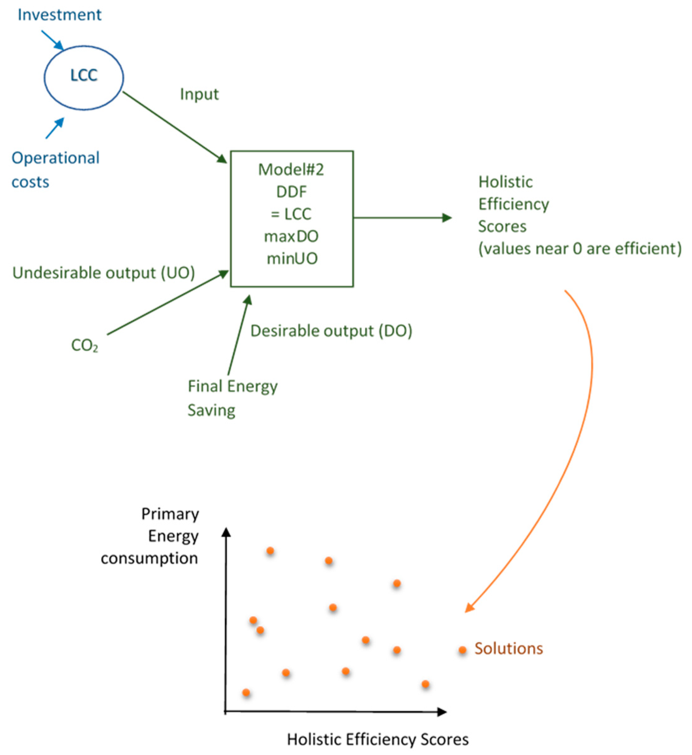
2.1. Method: The Directional Distance Function and the Bootstrap Resampling Technique

Following [10,28,29] the Directional Distance Function allows to obtain efficiency scores solving a linear programming not so different from the scores obtained by the standard data envelopment analysis approach (DEA). The directional function is defined to simultaneously minimize and maximize respectively inputs and outputs. The definition of the direction function is the following:

$$\overrightarrow{D}\left(\mathit{x},\mathit{y};-{\mathit{g}}_{\mathit{x}},{\mathit{g}}_{\mathit{y}}\right)=\sup \left\{\beta :\left(\mathit{x}-\beta {\mathit{g}}_{\mathit{x}},\mathit{y}+\beta {\mathit{g}}_{\mathit{y}}\right)\in P\right\}$$

The linear programming for the Directional Distance Function, when constant returns to scale (CRS) are assumed, is the following [28]:

$$\begin{array}{cc}\underset{\beta ,\lambda }{max}{\beta }_{CRS}^{*}\hfill & \\ \mathrm{subject}\mathrm{to}\hfill & \\ \mathrm{X}\lambda \le x_{\mathit{o}}-\beta {\mathit{g}}_{\mathit{x}}\hfill & \\ \mathit{Y}\lambda \ge y_{\mathit{o}}+\beta {\mathit{g}}_{\mathit{y}}\hfill & \\ \lambda \ge \mathbf{0}\hfill & \end{array}$$

(1)

where ${\beta }_{CRS}^{*}$ = 0, (i.e., a benchmark) represents the efficient observation, otherwise the score describes a situation of inefficiency. Indeed, increasing the efficiency scores (i.e., ${\beta }_{CRS}^{*}$ > 0), also inefficiency increases.

The biggest advantage of the DDF is the possibility to consider different types of outputs: from the one hand, the observation can produce a good output (in our case the final energy saving), but from the other hand, for producing the retrofitting intervention, the observation releases also emissions of CO₂ (b, bad or undesirable output). For this reason, the production possibility set has to be redefined in the following way:

$$P=\left\{\left(\mathit{x},{\mathit{y}}^{\mathit{d}},{\mathit{y}}^{\mathit{u}}\right)|\mathit{x}\ge X\mathit{\lambda },{\mathit{y}}^{\mathit{d}}\le Y\mathit{\lambda },{\mathit{y}}^{\mathit{u}}=Y\mathit{\lambda },\mathit{\lambda }\ge 0\right\}$$

Following [30], the undesirable outputs are weakly disposable and the efficiency scores represent the ability of the observation to reduce the bad output increasing the good one and taking inputs equal.

As the production set has changed, also the previous linear program has to be updated as follows [28]:

$$\begin{array}{cc}\underset{\beta ,\lambda }{max}{\beta }_{CRS}^{*}\hfill & \\ \mathrm{subject}\mathrm{to}\hfill & \\ \mathrm{X}\lambda \le x_{\mathit{o}}{}_{\mathit{x}}\hfill & \\ Y^d\lambda \ge {\mathit{y}}_{\mathit{o}}^{\mathit{d}}+\beta {\mathit{y}}_{\mathit{o}}^{\mathit{d}}\hfill & \\ Y^u\lambda \le {\mathit{y}}_{\mathit{o}}^{\mathit{u}}+\beta {\mathit{y}}_{\mathit{o}}^{\mathit{u}}\hfill & \\ & \max \left\{{\mathit{y}}_{\mathit{i}}^{\mathit{u}}\right\}\ge {\mathit{y}}_{\mathit{o}}^{\mathit{u}}+\beta {\mathit{y}}_{\mathit{o}}^{\mathit{u}}\hfill \\ & \lambda \ge \mathbf{0}\hfill \end{array}$$

(2)

Again, the optimal solution is ${\beta }_{CRS}^{*}$ = 0 and otherwise the observation is inefficient (i.e., ${\beta }_{CRS}^{*}$ > 0) (Efficiency scores vary between 0 and 1. Values equal to 0 represent the efficient observation, Increasing the scores, also inefficiency increases). Further, from the technical point of view, ref [11] suggest that the DDF frontier has to satisfy some axioms (inactivity, compactness of production possibility set, free disposability of inputs, weak disposability of outputs, null-jointness, free disposability of good outputs) that in the environmental case are always satisfied.

In addition, a resampling technique was applied to improve performance of non-parametric models and to obtain more robust efficiency scores [31,32].

The adopted resampling technique is the bootstrapping procedure that replicates n dataset starting from the initial sample. In the present paper, authors adopted the technique suggested by [33], applied until now in few studies [18,34,35].

Finally, notice that all elaborations (i.e., descriptive statistics, Directional Distance Functions, and bootstrap routine) were computed with the R-software version 4.0.1 (June 2020).

2.2. Data

Data used in the present work for creating the efficiency scores refer to the Packages of Optimal Solutions (POS) defined in the HAPPEN project implementation and collected in the report D3.4 [2] of the project, where they are freely disposable.

The project identifies 16 POS starting from four pilot case studies of deep retrofitting of residential buildings carried on in 4 different Countries. The Package of Optimal Solution (POS) is defined as a set of 12 solutions, each of which minimizes the LCC of the buildings after the renovation process with different combinations of technical renovation measures. Each POS was defined specifically for each reference building of the Country of the four pilot studies and for each climate zone (4 Countries and, for each Country, 4 climatic zones). The total 192 solutions referred to the 16 defined POS were formulated considering different combinations of renovation measures for the façades, for the renovation of the roofs, of the floors, of the thermal bridges, of the ventilation system, of the shading elements, and of different types of glazing [2].

The proposed analysis selected 2 different building typologies (i.e., 2 Single-Family Houses, SFH and 2 Multi-Family Houses, MFH) and 4 climate zones (i.e., W1S2; W2S2; W2S3; W3S2). The Single-Family Houses are homes including single- and two- family houses and terraced houses; the Multi-Family Houses refer to buildings with more than two apartments and fewer than 9 floors. Buildings that are higher than 8 floors are not considered in the present study (from the report D3.2 “Catalogue of reference buildings classes in MED countries”).

Considering the four-pilot case-studies analyzed, they are characterized by two main measures: the thermal transmittance $\widehat{U}$, (W/m²K) and the compactness C (m). In details: Cyprus: $\widehat{U}$ = 2.12 and C = 1.57; Labin: $\widehat{U }$= 2.23 and C = 1.33; Marseille: $\widehat{U }$= 1.89 and C = 3.46; Castéllon: $\widehat{U }$= 2.54 and C = 2.96 (data from the report [2]).

To identify the climate zones, the project considered both the Climate Severity Index (CSI) and the aim to cover the Mediterranean area. Different zones are identified with some acronyms where W means winter and S corresponds to summer (Climate zones were defined considering the Climate Severity Index equations for winter and for summer. In Appendix A,

Table A1. Climate zones based on thresholds of CSI.

Climate Zones	Winter	Summer
W1S1	0 ≤ CSI < 0.522	0 ≤ CSI < 0.508
W2S2	0.522 ≤ CSI < 1.52	0.508 ≤ CSI < 1.34
W2S3	0.522 ≤ CSI < 1.52	1.34 ≤ CSI < 2.00
W3S2	1.52 ≤ CSI < 2.77	0.508 ≤ CSI < 1.34

Source: data extracted from deliverable D3.1 “Report on representative climates and zoning”, Available online: https://ec.europa.eu/research/participants/documents/downloadPublic?documentIds=080166e5bc0b9398&appId=PPGMS (accessed on 7 November 2021).

reports details for the four climate zones considered). Croatia (HR) and Cyprus (CY) represent the pilots for SFH, while France (FR) and Spain (SP) are the front-runner pilots where the MFH typology was considered.

Table 1. Strategy design for Directional Distance Function estimation.

Building Typology	Climate Zone	Pilot Study (Country/POS n°)	Pilot Study (Country/POS n°)	Sample Size (Number of Solutions)	DDF Frontier
SFH	W1S2	CY (POS1)	HR (POS5)	24	1
	W2S2	CY (POS2)	HR (POS6)	24	2
	W2S3	CY (POS3)	HR (POS7)	24	3
	W3S2	CY (POS4)	HR (POS8)	24	4
MFH	W1S2	SP (POS13)	FR (POS9)	24	5
	W2S2	SP (POS14)	FR (POS10)	24	6
	W2S3	SP (POS15)	FR (POS11)	24	7
	W3S2	SP (POS16)	FR (POS12)	24	8

presents the strategy adopted for the DDF application. Indeed, considering each building typology and climate zone, 8 Directional Distance Functions were estimated. Let we consider, for instance, the MFH typology and the climate zone W1S2: 24 observations represent the sample size of DDF model (12 solutions for the corresponding POS13 from Spain and 12 solutions for the POS9 from France). The results are (holistic/environmental) efficiency scores that can be used for comparing the 24 solutions of each initial sample.

Indeed, the methodology proposed allows to obtain efficiency scores based on minimization of CO₂ emissions and the aim is to evaluate the efficiency of each solution for each POS considering the CO₂ emissions as a bad output.

With this intent, two model definitions were proposed, different for the input variables chosen. The outputs are two and they do not change in the two formulations. The final energy savings per year (The final energy savings per year (Mwh) represents the planned absolute value of the final energy savings per year) is the good output to maximize, while the CO₂ emissions (The CO₂ emissions represent the value of the CO₂ production after the implementation of the optimal solution proposed) represent the output to minimize (i.e., the bad or undesirable output). Concerning the inputs, the present paper proposes two formulations of the DDF estimations: the first one (Model#1) considers as input the LCC estimation for each solution; while Model#2 represents a more standard definition of the DDF, considering the total costs of solution.

The purpose to define two different input-output space strategies allows to consider different meanings of efficiency. In the case of Model#2, solutions are compared considering their ability to minimize the CO₂ emissions and simultaneously to maximize the final energy savings, using the same amount of costs. These results represent the environmental efficiency scores, well known in literature. However, thanks to the data collected in the HAPPEN project, scores with a more informative meaning were calculated considering the LCC as input. This happens in the Model#1, which considers not only the negative externalities of production process as bad output (i.e., emissions), but also costs and investments as input (LCC estimation). For this reason, the obtained results catch the holistic impact of the retrofitting interventions and allow to compare, in a simple way, different solutions.

All data used are available on the EU website of the project, and they were extracted from the [2]. The LCC is defined in the HAPPEN project as the initial investment plus the operational costs over 30 years after implementing the optimal solutions; and a deeper explanation of the computation can be found in [36]. In details, the Life-Cycle Costs are estimated as follows:

$$LCC(€)=Investment(€)+{\displaystyle \sum }_{i=1}^{30}\left(O{C}_i\right)·Discount rate$$

where OC represent the operational costs for each year expressed in €/year, and in this particular case, they refer to heating, cooling, energy consumptions, and maintenance costs.

The Discount Rate adopted is an annuity calculated as follows:

$$Discount rate=\frac{1-{\left(1+\raisebox{1ex}{$k$}\!\left/ \!\raisebox{-1ex}{$100$}\right.\right)}^{-30}}{k/100}$$

where the current interest rate k is 1.47%, calculated considering an interest rate of 3.5% and an inflation rate of 2% as suggested by the delegated regulation [37].

In addition, following [38], the size of input-output space (3 variables: 1 input + 2 outputs) allows to obtain robust results as an OLS with a sample equal to 69 units and the robustness of results is improved by the bootstrap resampling procedure.

Finally, we can sum up that the two input-output space strategies (Model#1: holistic efficiency, and Model#2: environmental efficiency) were used for defining the Directional Distance Functions considering the two building typologies (i.e., SFH and MFH), and the four climate zones (i.e., W1S2, W2S2, W2S3, W3S2). This means that 8 frontiers were built considering as input the Life-Cycle Cost estimations (Model#1), and 8 with total costs (Model#2). Notice that costs, as well as the final energy consumptions, vary significantly among climate zones (W1S2, W2S2, W2S3, W3S2), and different solutions of retrofitting interventions were analyzed separately. Descriptive statistics of input and outputs are presented in

Table 2. Input-output space descriptive statistics (mean values) (mean values are presented, but in model, all values for each solution of POS were used).

Building Typology	Input/ Output Space	Variables	W1S2	W2S2	W2S3	W3S2
SFH	Input (Model#1)	LCC (mean value, €/m2)	143.10	178.47	219.18	234.50
	Input (Model#2)	Total costs (€)	18,158	20,006	21,457	22,336
	Undesirable output	CO2 emissions (kg/m2)	9.24	12.25	16.15	17.12
	Good output	Final energy saving per year (Mwh)	13.50	21.57	25.45	36.94
MFH	Input (Model#1)	LCC (mean value, €/m2)	115.64	155.71	189.20	199.21
	Input (Model#2)	Total costs (€)	32,258	46,631	49,920	51,519
	Undesirable output	CO2 emissions (kg/m2)	8.81	10.75	14.05	14.97
	Good output	Final energy saving per year (Mwh)	31.69	33.80	41.05	58.94

.

3. Results and Discussion

Considering two different input-output spaces, results from Directional Distance Function are proposed with the aim to obtain two efficiency scores with two different meanings: Model#1 presents holistic scores, while Model#2 describes environmental efficiency scores. In both cases, scores equal to 0 represent the optimal observation that is placed on the efficient frontier. If the value of score increases, also the inefficiency grows.

Building typology and climate zone are the key variables used for presenting results with the aim to identify the more efficient solution(s) within the POS of each group.

3.1. Holistic and Environmental Efficiency Scores for Typology of Buildings in All the Climate Zones

Results of holistic and environmental efficiency scores are presented in

Table 3. Holistic and environmental efficiency scores (Model#1 and Model#2) for Single-Family House and all climate zones (CY = Cyprus and HR = Croatia).

SOLUTION	W1S2				W2S2				W2S3				W3S2
	MODEL#1		MODEL#2		MODEL#1		MODEL#2		MODEL#1		MODEL#2		MODEL#1		MODEL#2
	CY POS1	HR POS5	CY POS1	HR POS5	CY POS2	HR POS6	CY POS2	HR POS6	CY POS3	HR POS7	CY POS3	HR POS7	CY POS4	HR POS8	CY POS4	HR POS8
1	0.032	0.160	0.198	0.140	0.023	0.121	0.031	0.014	0.017	0.032	0.045	0.040	0.090	0.320	0.076	0.285
2	0.022	0.159	0.160	0.102	0.036	0.149	0.121	0.095	0.018	0.119	0.024	0.022	0.073	0.305	0.257	0.330
3	0.021	0.155	0.143	0.120	0.024	0.144	0.113	0.081	0.003	0.118	0.134	0.024	0.045	0.307	0.093	0.290
4	0.019	0.155	0.148	0.100	0.033	0.116	0.165	0.083	0.005	0.084	0.153	0.017	0.036	0.306	0.000	0.353
5	0.014	0.157	0.128	0.086	0.001	0.102	0.014	0.192	0.005	0.118	0.061	0.085	0.042	0.310	0.069	0.334
6	0.010	0.155	0.113	0.085	0.005	0.191	0.037	0.135	0.006	0.184	0.058	0.067	0.005	0.379	0.263	0.368
7	0.000	0.114	0.177	0.037	0.009	0.174	0.040	0.056	0.016	0.138	0.149	0.081	0.039	0.323	0.093	0.422
8	0.007	0.121	0.117	0.009	0.003	0.194	0.021	0.027	0.014	0.162	0.235	0.117	0.005	0.345	0.215	0.428
9	0.000	0.000	0.101	0.000	0.006	0.261	0.087	0.130	0.000	0.000	0.050	0.000	0.003	0.425	0.070	0.396
10	0.000	0.101	0.140	0.039	0.013	0.190	0.097	0.032	0.003	0.133	0.160	0.136	0.000	0.326	0.131	0.409
11	0.003	0.110	0.124	0.024	0.001	0.171	0.089	0.098	0.001	0.140	0.064	0.129	0.001	0.307	0.015	0.422
12	0.000	0.117	0.128	0.010	0.000	0.104	0.140	0.310	0.000	0.136	0.227	0.092	0.000	0.323	0.029	0.261

, where the building typology SFH is represented by the case-studies of Cyprus and Croatia (in particular, Labin). Table 3 shows the holistic and environmental scores (Model#1 and Model#2) for the 24 solutions referring to the different climate zones.

Considering the W1S2 climate zone, results suggest that solution 9 is the most efficient, both for holistic and environmental purposes. On the other hand, solution 1 presents the highest efficiency scores, suggesting that in all cases this is the most inefficient solution.

On the contrary, unclear conclusions can be obtained considering the W2S2 climate zone where solution 5 is always the most efficient in both holistic and environmental terms, except for the Model#2, case-study of Croatia, where the solution 1 presents the lowest environmental efficiency score.

Similar considerations can be carried on considering the W2S3 climate zone. Indeed, in this case, the solution 9 is the most efficient in holistic terms. Considering Model#2, solution 9 is the most efficient only for the Croatia case-study, indeed result for Cyprus suggests solution 2 as the best intervention. However, in this specific case, solution 9 does not present a high value of environmental efficiency, so we can conclude that the inefficiency for solution 9 is not too great in comparison to the best one (solution 2).

The results on W3S2 climate zone suggest that holistic efficiency solutions (Model#1) are the number 10 and 12 (Cyprus case-study), and solution 2 (Croatia). However, in general, efficiency values are very high. Environmental efficiency scores (Model#2) suggest that solutions 11 and 12 are the optimal choice for both case-studies, but in the case of Cyprus, solution 12 also does not present a too high environmental score.

Table 4. Holistic and environmental efficiency scores (Model#1 and Model#2) for Multi-Family House and all climate zones (FR = France and SP = Spain).

SOLUTION	W1S2				W2S2				W2S3				W3S2
	MODEL#1		MODEL#2		MODEL#1		MODEL#2		MODEL#1		MODEL#2		MODEL#1		MODEL#2
	FR POS9	SP POS13	FR POS9	SP POS13	FR POS10	SP POS14	FR POS10	SP POS14	FR POS11	SP POS15	FR POS11	SP POS15	FR POS12	SP POS16	FR POS12	SP POS16
1	0.022	0.242	0.069	0.376	0.013	0.004	0.413	0.776	0.053	0.007	0.552	0.132	0.026	0.068	0.582	0.048
2	0.020	0.151	0.151	0.211	0.022	0.253	0.322	0.143	0.064	0.087	0.498	0.056	0.045	0.051	0.549	0.160
3	0.015	0.132	0.032	0.174	0.018	0.274	0.403	0.197	0.043	0.140	0.535	0.097	0.038	0.029	0.645	0.022
4	0.005	0.122	0.087	0.150	0.018	0.169	0.357	0.062	0.056	0.083	0.511	0.818	0.059	0.024	0.643	0.040
5	0.000	0.089	0.187	0.125	0.009	0.060	0.232	0.243	0.018	0.143	0.305	0.058	0.021	0.063	0.369	0.064
6	0.011	0.074	0.046	0.064	0.004	0.238	0.370	0.012	0.009	0.114	0.455	0.023	0.009	0.041	0.038	0.038
7	0.000	0.045	0.043	0.029	0.017	0.068	0.483	0.277	0.000	0.094	0.033	0.047	0.035	0.048	0.615	0.092
8	0.000	0.000	0.000	0.000	0.021	0.294	0.509	0.000	0.023	0.136	0.505	0.000	0.015	0.077	0.467	0.195
9	0.000	0.095	0.008	0.074	0.000	0.158	0.351	0.086	0.000	0.072	0.445	0.055	0.045	0.020	0.662	0.089
10	0.000	0.060	0.062	0.028	0.000	0.036	0.322	0.301	0.006	0.092	0.410	0.074	0.060	0.032	0.660	0.132
11	0.004	0.141	0.009	0.095	0.011	0.081	0.461	0.078	0.021	0.019	0.507	0.049	0.002	0.123	0.236	0.938
12	0.005	0.132	0.115	0.076	0.004	0.107	0.367	0.059	0.029	0.113	0.445	0.001	0.021	0.075	0.522	0.059

presents results on Multi-Family House (MFH) in France and Spain (in particular, the front-runner pilots are in Marseille and in Castellòn). The presented analysis is equal to the previous one on Single-Family House and 8 Directional Distance Functions were run considering the two different formulation of input-output space and the four climate zones.

As in the case of SFH, considering the W1S2 climate zone, a univocal solution always presents the best results in terms of both holistic and environmental efficiency. This solution is the number 8 but considering the Model#1 and the Marseille case study, there are many holistic efficiency solutions.

Taking W2S2 and W2S3 climate zones into account, results are controversial. Indeed, in the first case (W2S2), both Model#1 and Model#2 suggest different efficient solutions. Less controversial conclusions can be found for W2S3 climate zone: both models suggest solution 7 as the best for Marseille, whereas for Castellòn there is not a univocal solution, but it changes on the base of the model adopted.

Finally, also for the W3S2 climate zone conclusions on results are not so clear. However, for France and considering the holistic efficiency, solution 6 is clearly the best choice, whereas in other cases Model#1 and Model#2 suggest more than one (holistic and environmental) efficient solution.

The models proposed present not always univocal results, even if scores suggest which is the best solution for each country. This means that, to decide which could be the optimal choice, in next subsection we propose to cross in a Cartesian coordinate system, the obtained results of holistic efficiency scores with other variables that can suggest definitely the optimal solution.

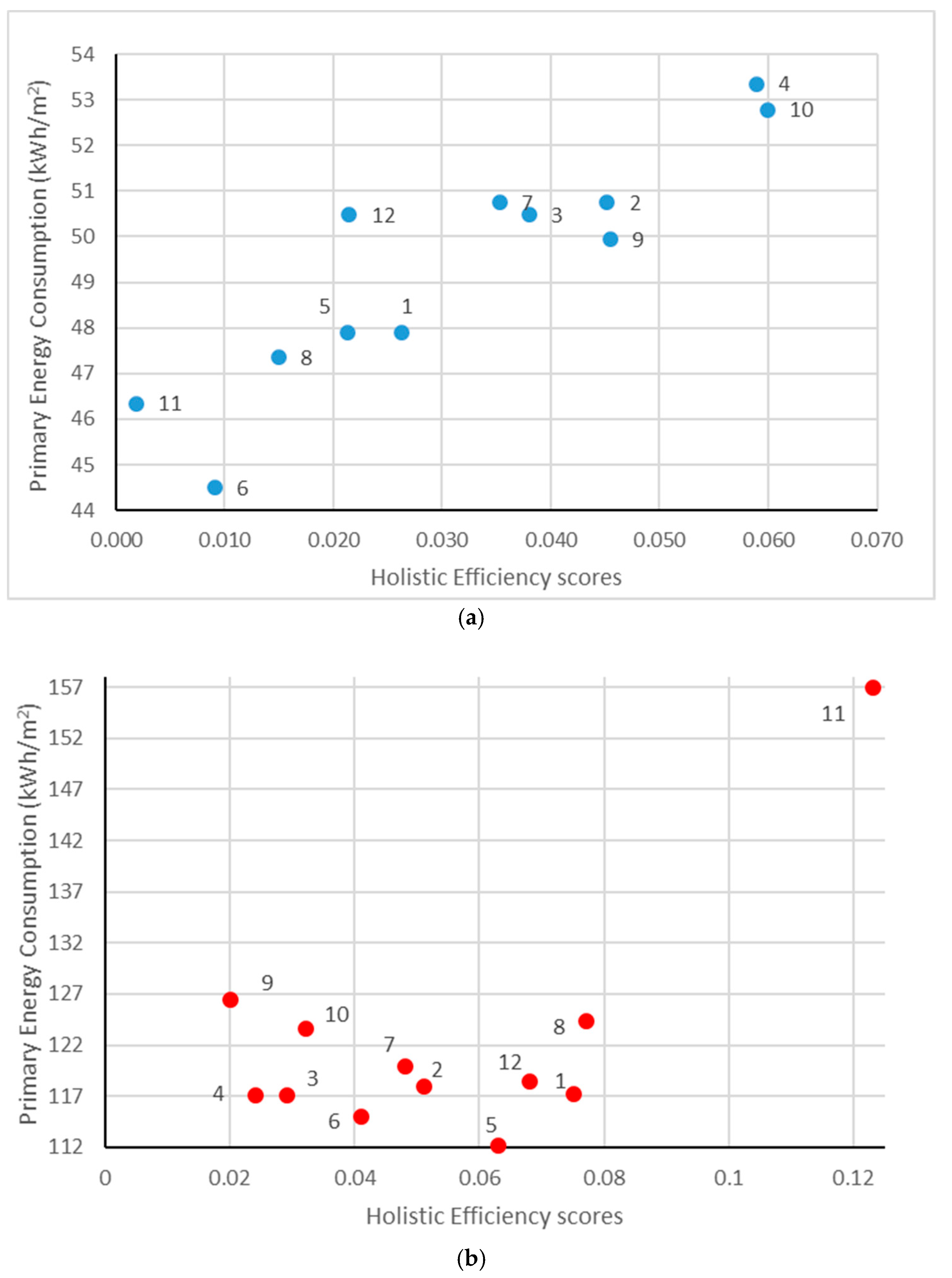
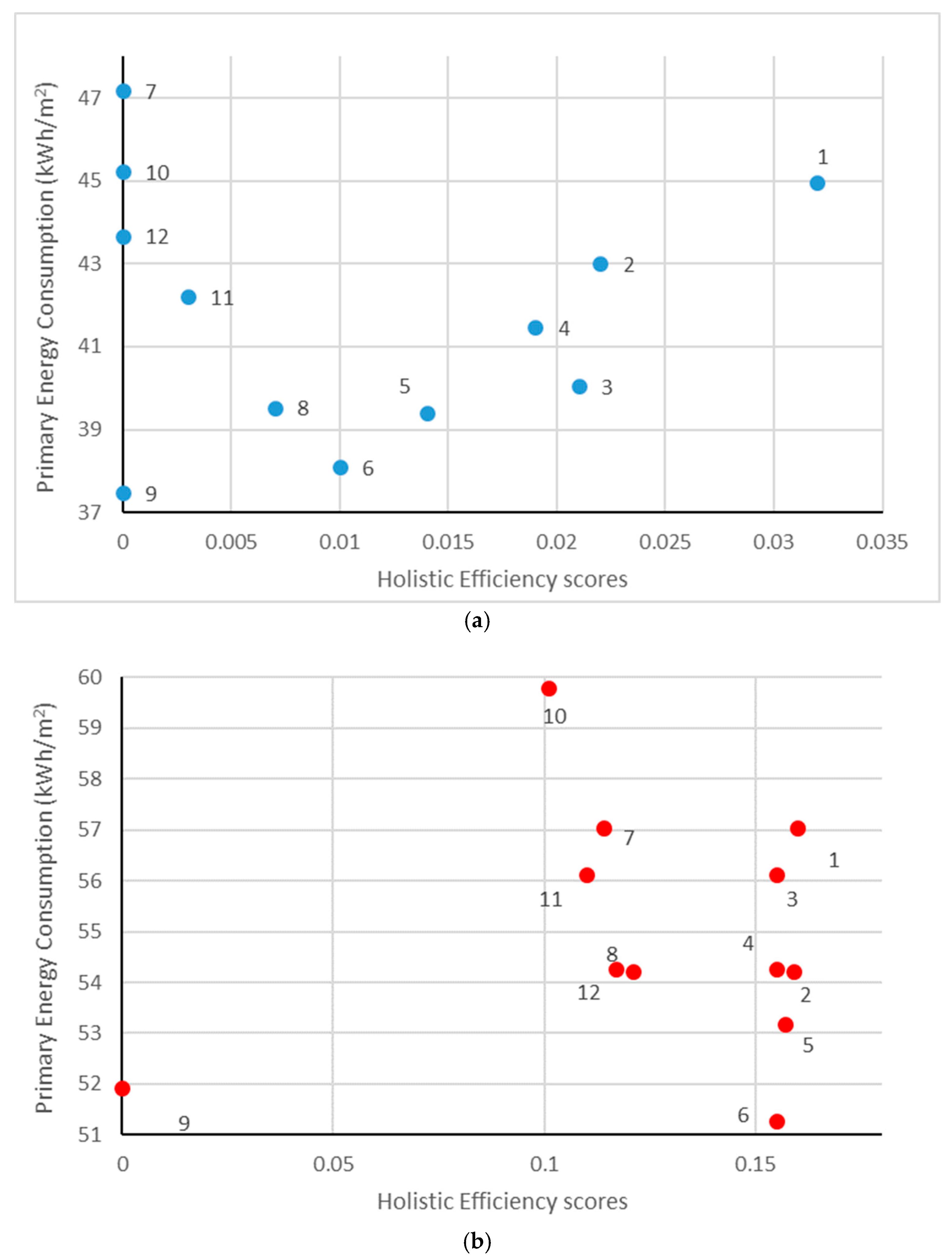
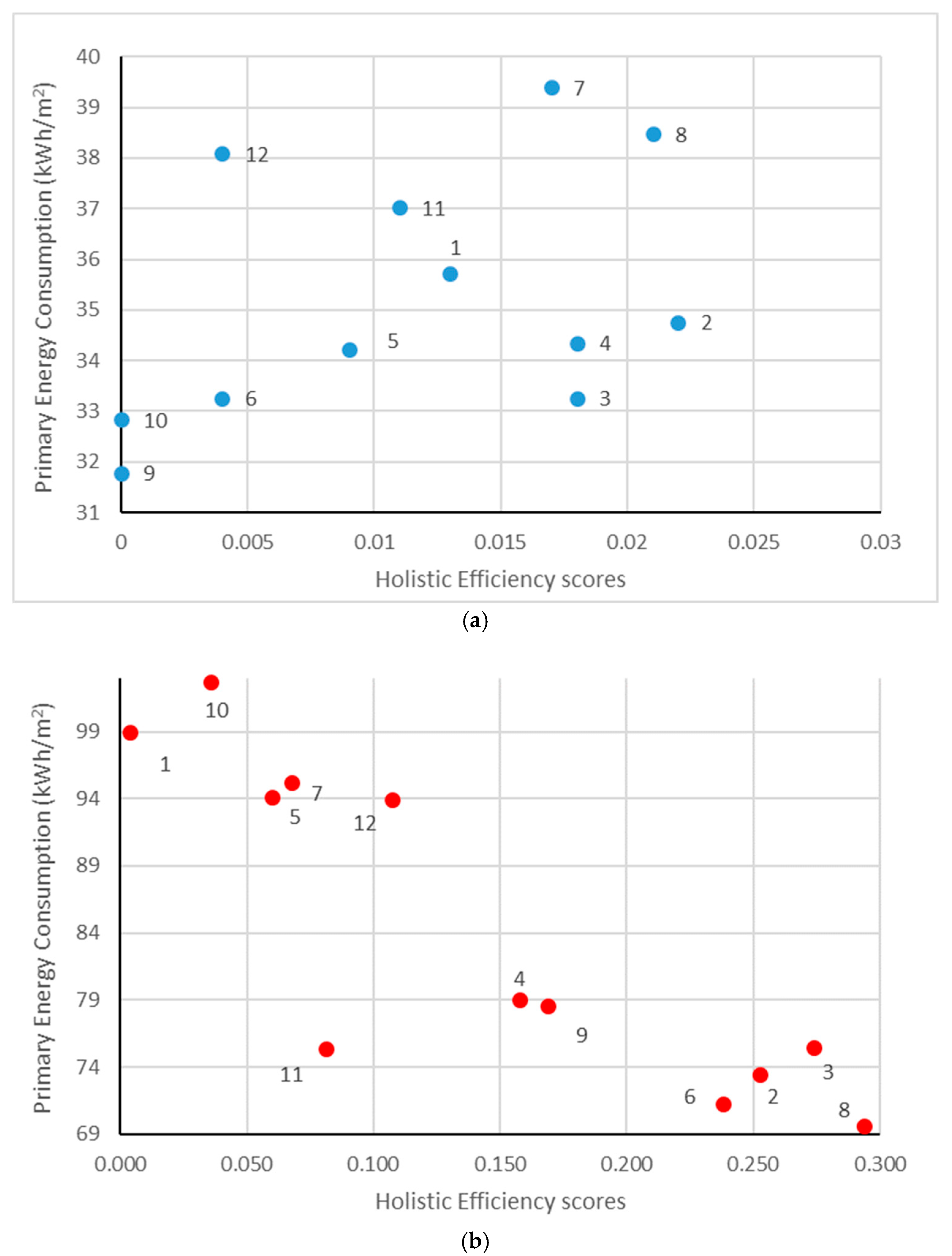
3.2. How to Choose the Optimal Solution within Each POS?

To discuss and clarify the previous results, it is interesting to consider both the holistic efficiency scores (Model#1) together with some characteristics of the solutions. We decided to used Model#1 because the holistic efficiency scores represent a more complete definition of efficiency and the decision of customer is to decide which intervention is the most convenient from different point of views. Scores from Model#2 are also relevant, but they refer specifically to environmental issues. Indeed, for instance, they do not take into account the size of investment that, on the contrary, is considered in LCC estimations used in Model#1.

Table 5. Primary Energy Consumption (kWh/m²) and Life Cycle Cost (€/m²) for solutions of Single-Family Houses in climate zones.

Solutions	W1S2				W2S2				W2S3				W3S2
	Primary Energy Consumption (kWh/m2)		LCC (€/m2)		Primary Energy Consumption (kWh/m2)		LCC (€/m2)		Primary Energy Consumption (kWh/m2)		LCC (€/m2)		Primary Energy Consumption (kWh/m2)		LCC (€/m2)
	CY POS1	HR POS5	CY POS1	HR POS5	CY POS2	HR POS6	CY POS2	HR POS6	CY POS3	HR POS7	CY POS3	HR POS7	CY POS4	HR POS8	CY POS4	HR POS8
1	44.95	57.05	123.31	150.60	56.64	88.89	156.18	194.44	69.75	80.06	200.82	231.29	80.80	104.60	211.03	237.47
2	43.00	54.22	125.07	152.50	59.89	92.34	156.45	194.70	68.45	66.12	200.85	233.13	89.20	108.41	218.30	240.79
3	40.04	56.13	125.49	153.92	60.23	94.30	158.02	195.69	80.26	69.15	201.00	233.62	86.69	106.72	220.60	240.94
4	41.47	54.26	126.11	154.74	63.43	90.46	158.22	195.78	81.63	83.26	201.11	233.97	81.07	109.30	222.06	241.11
5	39.41	53.18	126.63	155.61	50.58	97.68	160.87	196.39	73.58	89.54	202.16	235.34	85.44	108.81	222.33	242.14
6	38.09	51.27	127.20	156.37	47.51	93.90	160.89	196.46	72.29	85.09	202.21	235.80	94.95	110.47	227.49	244.16
7	47.18	57.05	127.26	161.75	53.83	97.00	162.08	196.46	84.21	75.49	202.56	236.26	89.47	112.96	229.32	244.19
8	39.53	54.22	127.84	163.65	50.75	95.86	162.11	196.72	85.56	71.14	202.63	236.27	93.76	111.40	229.39	244.56
9	37.47	51.92	128.34	164.04	60.30	86.22	162.31	196.81	72.72	81.46	203.97	236.92	78.05	110.88	230.46	245.51
10	45.22	59.79	128.98	164.70	63.56	102.04	162.60	196.94	84.74	67.46	204.54	237.97	75.79	113.36	230.87	245.53
11	42.21	56.13	129.36	165.07	63.89	99.23	164.18	197.13	76.50	78.32	205.23	237.98	86.97	115.01	231.64	247.53
12	43.67	54.26	130.03	165.89	67.11	98.45	164.39	197.35	88.62	92.52	205.97	238.74	91.34	104.60	231.91	248.62

Source: Elaboration from the Deliverable 3.4 and Annexes, HAPPEN Project, D3.4—Calculations on Reference Buildings and Identification of Optimal Integrated Packages of Solutions. Available online: https://ec.europa.eu/research/participants/documents/downloadPublic?documentIds=080166e5ccfa6591&appId=PPGMS (accessed on 6 November 2021).

and

Table 6. Primary Energy Consumption (kWh/m²) and Life Cycle Cost (€/m²) for solutions of Multi-Family Houses in climate zones.

Solutions	W1S2				W2S2				W2S3				W3S2
	Primary Energy Consumption (kWh/m2)		LCC (€/m2)		Primary Energy Consumption (kWh/m2)		LCC (€/m2)		Primary Energy Consumption (kWh/m2)		LCC (€/m2)		Primary Energy Consumption (kWh/m2)		LCC (€/m2)
	FR POS9	SP POS13	FR POS9	SP POS13	FR POS10	SP POS14	FR POS10	SP POS14	FR POS11	SP POS15	FR POS11	SP POS15	FR POS12	SP POS16	FR POS12	SP POS16
1	37.94	53.59	88.24	126.69	35.72	98.97	115.21	179.60	47.89	98.92	134.84	230.05	47.90	118.51	133.17	250.20
2	41.40	49.47	88.55	128.30	34.76	73.47	115.30	180.76	49.84	94.67	135.40	233.93	50.77	118.01	133.51	250.72
3	36.75	48.95	88.90	129.78	33.26	75.50	115.82	186.37	45.76	100.29	135.52	234.32	50.49	117.20	134.61	260.84
4	40.59	50.52	89.81	133.05	34.35	78.60	115.93	192.47	47.71	127.89	136.08	235.62	53.36	117.16	134.98	261.04
5	44.06	48.57	90.15	136.38	34.22	94.14	117.03	194.81	43.17	95.80	138.16	236.52	47.90	112.24	135.62	261.71
6	38.09	51.59	90.25	143.27	33.26	71.29	117.12	195.15	44.24	97.33	138.79	239.44	44.52	115.12	135.66	262.66
7	39.39	51.52	90.45	145.19	39.40	95.20	117.30	195.91	41.03	104.86	138.80	243.34	50.77	120.00	135.97	264.77
8	36.78	47.16	90.49	145.40	38.47	69.59	117.48	195.93	45.18	96.23	138.84	243.47	47.36	124.40	135.98	265.16
9	37.64	55.90	90.56	148.95	31.78	79.04	117.66	200.07	42.08	94.68	139.40	244.54	49.96	126.56	136.32	266.57
10	40.22	53.45	90.78	151.27	32.84	102.70	117.74	201.91	43.03	104.67	139.46	245.77	52.80	123.67	136.61	267.87
11	36.84	64.95	90.81	152.93	37.02	75.37	118.07	202.68	46.25	104.50	139.46	249.33	46.35	157.03	136.96	269.14
12	41.70	64.95	90.88	154.34	38.09	93.92	118.13	208.58	49.70	122.54	140.02	249.70	50.49	117.22	137.06	273.84

Source: Elaboration from the Deliverable 3.4 and Annexes, HAPPEN Project, D3.4—Calculations on Reference Buildings and Identification of Optimal Integrated Packages of Solutions. Available online: https://ec.europa.eu/research/participants/documents/downloadPublic?documentIds=080166e5ccfa6591&appId=PPGMS (accessed on 6 November 2021).

report, respectively for Single-Family and Multi-Family houses, the amounts of Primary Energy Consumption (kWh/m²) (The primary energy consumption is the value of energy consumption of the buildings (for each m²) after the implementation of the optimal solution (as defined in report D3.4 of the HAPPEN Project) [2]) and of Life Cycle Cost (€/m²) for each solution and climate zone. Data were elaborated from the Deliverable 3.4 of HAPPEN project and the Life Cycle Cost methodology was presented in [36].

To calculate the LCC estimates, the initial investment is considered and, at the same time, the LCC was used as input for the Model#1 applied for computing the holistic efficiency of solutions. On the contrary, the primary energy consumption could were an input for the frontiers, because, together with the LCC, are key variables in finding the optimal solution. However, the sample size does not allow to obtain robust results with an input-output space bigger than that used. For this reason, in both models the good output to maximize was represented by the final energy saving that, together with CO₂ emissions, is the most suitable candidate to catch the effects on consumptions.

From the analysis, we can observe that, in general, the obtained efficiency scores do not always match with the minimum values of primary energy consumption.

Indeed, considering the case of Single-Family house and W1S2 climate zone, the solution 9 is the best in terms of efficiency (Table 3); however, considering Table 5, it does not correspond to the minimum LCC evaluation, but it is the best solution considering the primary energy consumption. Indeed, the proposed scores measure which solution has the minimum impact on environment, in terms of CO₂, and the maximum capacity in final energy saving, taking equal the LCC (Model#1) or total costs (Model#2). We could conclude that results are contradictory but in truth the meaning of LCC alone and of efficiency scores is different. However, results in Table 5 suggest that considering only LCC, the solution 9 is not the best one (i.e., solution 9 does not present the lowest level of LCC for W1S2 climate zone), but the solution 9 is the most efficient considering the LCC together with the impact in terms of energy savings and emissions (i.e., from Table 3, solution 9 presents the lowest efficiency scores). For this reason, the methodology proposed presents the most complete evaluation of solutions, considering not only costs and investments, but also negative externalities (i.e., CO₂ emissions).

Considering this specific case (W1S2), from Table 5 solution 1 (POS1 and POS5) presents the lower LCC values but Table 3 (Model#1) suggests that this solution is not the most efficient because the efficiency score is higher than 0, rather it is the worst in terms of produced outputs and also the primary energy consumption is very high compared with that of other alternatives.

Similar results are obtained in the case of multifamily houses and W1S2 climate zone (Table 4 Model#1 and Table 6). Indeed, also in this case, models agree in highlighting solution 8 (POS9 and POS13) as the more efficient. Table 6 shows that this solution does not present the minimum value of LCC estimation but in terms of initial energy consumption is the best choice.

Nevertheless, considering all results of efficient frontiers and values of primary energy consumptions, it is not so clear which solution is able to combine all factors affecting the choice to do retrofitting interventions.

For this reason and to explain better the results, we propose the scatterplots for each typology of building and climate zone, where the efficiency scores, calculated with LCC (i.e., holistic efficiency scores, Model#1) represent the values on abscissa axis and the values of the primary energy consumption are placed on ordinate axis.

Figure 1 presents the methodology applied: we have used the LCC estimation as input for the estimation of DDF with CO₂ emissions as undesirable output and the final energy saving as desirable one. Results are holistic efficiency scores representing the capability of solution to minimize emission and maximizing the final energy saving (taking equal the LCC). Finally, we crossed these scores with the primary energy consumption that is another crucial variable to consider in the choice of retrofitting interventions.

These figures with scatterplots allow to evaluate the best solution considering the holistic efficiency scores and the primary energy consumptions. These representations clearly suggest choosing the solutions near to the origin of axes where the holistic efficiency is at its maximum and the primary energy consumption is at its minimum. The bullet points in the figures represent the solutions of each POS, as described in the near labels.

Figure 2 shows the plot referring to the Single-Family houses and climate zone W1S2. In this case the graph confirms previous considerations and for Cyprus the solution 9 (POS1) is the best one as in the case of Croatia (POS5).

Figure 3 considers W2S2 climate zone and if for Cyprus solutions 5, 6, and 8 of POS2 can be considered as optimal; on the contrary, Croatia presents an optimal combination of efficiency scores and consumptions for solution 1 of POS6, confirming results obtained in previous analysis.

Figure 4 shows that optimal solution for W2S3 climate zone for Cyprus is the number 9 of POS3, whereas for Croatia, the optimal solution is the number 1 of POS7. Considering the last climate zone (i.e., W3S2), Figure 5 suggests that for the first considered pilot (Cyprus) the solution 10 is the best possible choice of POS4, whereas for Croatia the best is the number 1 (POS8).

The same analysis was carried out for the case-studies referring to multifamily houses (i.e., France and Spain).

As suggested, for the first climate zone (i.e., W1S2) the choice of the optimal solution is univocally identified in the solution number 8 of POS9 and POS13 (Figure 6). For climate zone W2S2, Figure 7 shows that for France the best choice of intervention is the number 9 (POS10); for the second front-runner pilot (i.e., Spain), the optimal solution is the number 11 (POS14).

Figure 8 presents results for the W2S3 climate zone where the solution 7 of POS11 is the optimal intervention for France, while in the second case-study (i.e., Spain), solution 1 of POS15 results to be the best choice.

Finally, considering the climate zone W3S2, Figure 9 for France highlights solutions 6 and 11 of POS12 as the optimal retrofitting interventions, whereas for Spain the solution 4 of POS16 is the nearest to the origin of axis.

4. Conclusions

Starting from data collected in HAPPEN project [2], we propose an innovative application of a well-known methodology for computing the efficiency of retrofitting interventions on the building stock of the Mediterranean area, considering their economic and environmental spillovers. Indeed, the method used, the Directional Distance Function, allows to obtain an efficiency score representing the solution that minimizes the CO₂ emissions and, at the same time, maximizes the saving of final energy consumptions.

The paper presents two model formulations, to show the potentiality of the approach. Indeed, through Model#1, authors propose an evaluation of the holist efficiency because the Life Cycle Costing estimation is introduced as input; instead, a classical environmental efficiency was also estimated using as input the total cost of the interventions. The main purpose of the present experiment is to propose a simple tool that, considering few variables, is able to give a score easy to interpret in terms of efficiency.

A methodology frequently applied for evaluating the impact on social and health systems due to a production process (e.g., the retrofitting interventions on buildings) is the Life-Cycle Assessment (i.e., LCA) that is recognized as an appropriate methodology. However, a high availability of data is necessary for computing the LCA; in this work, we propose a combination of LCC and Directional Distance Function as a simpler methodology for evaluating which solutions for each typology of building and climate zone are more efficient. Then, the paper presents an alternative methodology simpler than those suggested by the majority of literature to evaluate the optimal choice.

The method proposed can be useful for all stakeholders of a retrofitting investments in different phases. From the one hand, the hybrid-DDF methodology can be used before starting the investment, because considering different scenarios, as it was made in the project, the methodology identifies the more efficient solution for each typology of building and for each climate zone. Nevertheless, also during the interventions, investors can compare easily different solutions and choose the more efficient from the costs point of view. In addition, in this definition of the model, the information on the initial investment is considered also thanks to the LCC estimation, then the investor will be able to estimate which solution is the most attractive alternative for him.

Last but not least, the correct evaluation of retrofitting interventions is very crucial when the building to retrofit was built before the 1945 (so called “historic buildings”). As suggested by [39], the retrofitting of historic buildings can be very expensive but, at the same time, the spillovers in term of market value can be a key-variable in the decision for the intervention. However, in large part, historic buildings are cultural heritage and, for example in Italy, the interventions are not attractive from the economic point of view [39]. This evidence is supported also by [40] that identifies two main reasons: restrictions imposed by the authorities for the preservation of cultural heritage, and the exclusion of historic buildings from conventional public policies. Starting from these considerations, [40] proposes a methodology able to evaluate the choice between the energy performance and cultural value (an interesting review of problems related to the comparison between retrofitting traditional and historic buildings can be found in [41]. A reference for legislative and regulatory aspects of historic building retrofitting is in [42]).

Even if the Directional Distance Function is quite easy to calculate and results are very evident, the methodology presents some weaknesses. The main one concerns the choice of variables for the computation of scores. Indeed, many factors can affect the efficiency of a retrofitting intervention, and limiting the choice to only 3 variables probably does not allow to obtain the best possible efficiency score. However, the number of inputs and outputs is strictly connected to the sample size. As suggested by literature [38], if we want to increase the input-output dimension, it is necessary to increase the sample size. It is for this reason that, in the present paper, we suggest a hybrid methodology considering also other characteristics of retrofitting building and, it could be interesting, to define a composite indicator able to evaluate the intervention in the whole.

Finally, it is necessary to better explain that in the paper is proposed a methodology for supporting the decision maker. The aim of the paper is twofold: from the one hand, we fill the gap existing in retrofitting intervention evaluation proposing a hybrid methodology and, from the other hand, we propose a simple tool for ranking renovation solutions considering together an efficiency score and other crucial measure for retrofitting interventions, as in this case the primary energy consumption. Obtained results cannot be compared with other ones, because the final choice of the best solution, between those proposed for each POS, strictly depends from the investors and the specific objectives they pursue that will lead them to choose or not the suggested solutions. Our methodology is a tool for the decision making because it was able to consider together a composite indicator of efficiency and, at the same time, at least another relevant variable, but it remains a suggestion, which the investor will evaluate on the basis of his objectives.

Next step will be to use a bigger sample of solutions to make possible the introduction of new variables in the input-output space and to create a hybrid composite indicator of efficiency more significant. In addition, the idea to create hybrid models is supported by literature suggesting that combined approaches can be very useful in defining criteria for decision analysis in sustainability assessment [43,44,45,46]. In both cases, the aim is to obtain richer results able to help investors, customers, and in general all stakeholders to take the best decision from economic, social, and environmental point of view.

References

1. European Commission. (15 April 2019), New Rules for Greener And Smarter Buildings Will Increase Quality of Life for All Europeans. Available online: https://ec.europa.eu/info/news/new-rules-greener-and-smarter-buildings-will-increase-quality-life-all-europeans-2019-apr-15_en (accessed on 3 November 2021).
2. Salmeron Lissen, J.M. (2020) D3.4—Calculations on Reference Buildings and Identification of Optimal Integrated Packages of Solutions. Available online: https://ec.europa.eu/research/participants/documents/downloadPublic?documentIds=080166e5ccfa6591&appId=PPGMS (accessed on 6 November 2021).
3. EUR-Lex. Access to European Union Law. Available online: https://eur-lex.europa.eu/LexUriServ/LexUriServ.do?uri=OJ:L:2012:081:0018:0036:EN:PDF (accessed on 3 November 2021).
4. Chung, Y.; Färe, R.; Grosskopf, S. Productivity and Undesirable Outputs: A Directional Distance Function Approach. J. Environ. Manag. 1997, 51, 229–240. [Google Scholar] [CrossRef] [Green Version]
5. Faere, R.; Grosskopf, S.; Lovell, C.A.K.; Pasurka, C. Multilateral Productivity Comparisons When Some Outputs are Undesirable: A Nonparametric Approach. Rev. Econ. Stat. 1989, 71, 90. [Google Scholar] [CrossRef]
6. Zofío, J.L.; Prieto, A.M. Environmental efficiency and regulatory standards: The case of CO2 emissions from OECD industries. Resour. Energy Econ. 2001, 23, 63–83. [Google Scholar] [CrossRef]
7. Ball, V.E.; Lovell, C.A.K.; Luu, H.; Nehring, R. Incorporating environmental impacts in the measurement of agricultural productivity growth. J. Agric. Resour. Econ. 2004, 29, 436–460. [Google Scholar]
8. Cuesta, R.A.; Zofío, J.L. Hyperbolic Efficiency and Parametric Distance Functions: With Application to Spanish Savings Banks. J. Prod. Anal. 2005, 24, 31–48. [Google Scholar] [CrossRef]
9. Chambers, R.G.; Chung, Y.; Färe, R. Benefit and Distance Functions. J. Econ. Theory 1996, 70, 407–419. [Google Scholar] [CrossRef]
10. Chambers, R.G.; Chung, Y.; Färe, R. Profit, Directional Distance Functions, and Nerlovian Efficiency. J. Optim. Theory Appl. 1998, 98, 351–364. [Google Scholar] [CrossRef]
11. Färe, R.; Grosskopf, S.; Pasurka, C.A. Environmental production functions and environmental directional distance functions. Energy 2007, 32, 1055–1066. [Google Scholar] [CrossRef]
12. McMullen, B.S.; Noh, D.-W. Accounting for emissions in the measurement of transit agency efficiency: A directional distance function approach. Transp. Res. Part D Transp. Environ. 2007, 12, 1–9. [Google Scholar] [CrossRef]
13. Kumar, S.; Managi, S. Sulfur dioxide allowances: Trading and technological progress. Ecol. Econ. 2010, 69, 623–631. [Google Scholar] [CrossRef]
14. Kumar, S.; Managi, S. Environment and productivities in developed and developing countries: The case of carbon dioxide and sulfur dioxide. J. Environ. Manag. 2010, 91, 1580–1592. [Google Scholar] [CrossRef]
15. Zhang, C.; Liu, H.; Bressers, H.T.; Buchanan, K.S. Productivity growth and environmental regulations—Accounting for undesirable outputs: Analysis of China’s thirty provincial regions using the Malmquist–Luenberger index. Ecol. Econ. 2011, 70, 2369–2379. [Google Scholar] [CrossRef]
16. Falavigna, G.; Manello, A.; Pavone, S. Environmental efficiency, productivity and public funds: The case of the Italian agricultural industry. Agric. Syst. 2013, 121, 73–80. [Google Scholar] [CrossRef]
17. Falavigna, G.; Ippoliti, R. The socio-economic planning of a community nurses programme in mountain areas: A Directional Distance Function approach. Socio-Econ. Plan. Sci. 2019, 71, 100770. [Google Scholar] [CrossRef]
18. Falavigna, G.; Ippoliti, R.; Manello, A.; Ramello, G.B. Judicial productivity, delay and efficiency: A Directional Distance Function (DDF) approach. Eur. J. Oper. Res. 2015, 240, 592–601. [Google Scholar] [CrossRef]
19. Ibáñez-Forés, V.; Bovea, M.D.; Pérez-Belis, V. A holistic review of applied methodologies for assessing and selecting the optimal technological alternative from a sustainability perspective. J. Clean. Prod. 2014, 70, 259–281. [Google Scholar] [CrossRef]
20. Álvarez-Rodríguez, C.; Martín-Gamboa, M.; Iribarren, D. Combined use of Data Envelopment Analysis and Life Cycle Assessment for operational and environmental benchmarking in the service sector: A case study of grocery stores. Sci. Total. Environ. 2019, 667, 799–808. [Google Scholar] [CrossRef] [PubMed]
21. Pishgar-Komleh, S.H.; Żyłowski, T.; Rozakis, S.; Kozyra, J. Efficiency under different methods for incorporating undesirable outputs in an LCA+DEA framework: A case study of winter wheat production in Poland. J. Environ. Manag. 2020, 260, 110138. [Google Scholar] [CrossRef] [PubMed]
22. Zhu, L.; Liu, J.; Xie, J.; Yu, Y.; Gao, L.; Li, S.; Duan, H. Can efficiency evaluation be applied to power plant operation improvement? A combined method with modified weighted russell directional distance model and pattern matching. Comput. Oper. Res. 2021, 134, 105406. [Google Scholar] [CrossRef]
23. Liu, X.; Chu, J.; Yin, P.; Sun, J. DEA cross-efficiency evaluation considering undesirable output and ranking priority: A case study of eco-efficiency analysis of coal-fired power plants. J. Clean. Prod. 2017, 142, 877–885. [Google Scholar] [CrossRef]
24. Joint Research Centre-European Commission. Handbook on Constructing Composite Indicators: Methodology and User Guide; Organisation for Economic Co-operation and Development: Paris, France, 2008; ISBN 978-92-64-04345-9. [Google Scholar]
25. Dobos, I.; Vörösmarty, G. Green supplier selection and evaluation using DEA-type composite indicators. Int. J. Prod. Econ. 2014, 157, 273–278. [Google Scholar] [CrossRef]
26. Andreolli, F.; Bragolusi, P.; D’Alpaos, C.; Faleschini, F.; Zanini, M.A. An AHP model for multiple-criteria prioritization of seismic retrofit solutions in gravity-designed industrial buildings. J. Build. Eng. 2021, 45, 103493. [Google Scholar] [CrossRef]
27. Yang, L.; Ma, C.; Yang, Y.; Zhang, E.; Lv, H. Estimating the regional eco-efficiency in China based on bootstrapping by-production technologies. J. Clean. Prod. 2019, 243, 118550. [Google Scholar] [CrossRef]
28. Falavigna, G.; Ippoliti, R. Reform policy to increase the judicial efficiency in Italy: The opportunity offered by EU post-Covid funds. J. Policy Model. 2021, 43, 923–943. [Google Scholar] [CrossRef]
29. Färe, R.; Grosskopf, S. Theory and Application of Directional Distance Functions. J. Prod. Anal. 2000, 13, 93–103. [Google Scholar] [CrossRef]
30. Cooper, W.W.; Seiford, L.M.; Tone, K. Data Envelopment Analysis: A Comprehensive Text with Models, Applications, References and DEA-Solver Software; Princeton University Press: Princeton, NJ, USA, 2007. [Google Scholar]
31. Simar, L.; Wilson, P.W. Sensitivity Analysis of Efficiency Scores: How to Bootstrap in Nonparametric Frontier Models. Manag. Sci. 1998, 44, 49–61. [Google Scholar] [CrossRef] [Green Version]
32. Simar, L.; Wilson, P.W. Estimation and inference in two-stage, semi-parametric models of production processes. J. Econ. 2007, 136, 31–64. [Google Scholar] [CrossRef]
33. Chernick, M.R. Bootstrap Methods: A Guide for Practitioners and Researchers; John Wiley & Sons: Hoboken, NJ, USA, 2011; Volume 619. [Google Scholar]
34. Falavigna, G.; Manello, A. The influence of financial and technological structure on eco-efficiency: An application of DDF bootstrapped framework in the Italian polluting industries. Int. J. Comput. Econ. Econom. 2021. Accepted paper, forthcoming. [Google Scholar]
35. Riquelme, J.N.F.; Meré, J.B.O.; Zinilli, A.; Reale, E. The Proposal of a New Hybrid Methodology for the Impact Assessment of Energy Efficiency Interventions. An Exploratory Study; CNR-IRCrES Working Paper; Istituto di Ricerca sulla Crescita Economica Sostenibile: Roma, Italy, 2020. [Google Scholar] [CrossRef]
36. Lissen, J.S.; Escudero, C.J.; De La Flor, F.S.; Escudero, M.; Karlessi, T.; Assimakopoulos, M.-N. Optimal Renovation Strategies through Life-Cycle Analysis in a Pilot Building Located in a Mild Mediterranean Climate. Appl. Sci. 2021, 11, 1423. [Google Scholar] [CrossRef]
37. de Vasconcelos, A.B.; Pinheiro, M.D.; Manso, A.; Cabaço, A. EPBD cost-optimal methodology: Application to the thermal rehabilitation of the building envelope of a Portuguese residential reference building. Energy Build. 2016, 111, 12–25. [Google Scholar] [CrossRef]
38. Wilson, P.W. Dimension reduction in nonparametric models of production. Eur. J. Oper. Res. 2018, 267, 349–367. [Google Scholar] [CrossRef]
39. Filippi, M. Remarks on the green retrofitting of historic buildings in Italy. Energy Build. 2015, 95, 15–22. [Google Scholar] [CrossRef]
40. Onecha, B.; Dotor, A.; Marmolejo-Duarte, C. Beyond Cultural and Historic Values, Sustainability as a New Kind of Value for Historic Buildings. Sustainability 2021, 13, 8248. [Google Scholar] [CrossRef]
41. Webb, A.L. Energy retrofits in historic and traditional buildings: A review of problems and methods. Renew. Sustain. Energy Rev. 2017, 77, 748–759. [Google Scholar] [CrossRef]
42. Mazzarella, L. Energy retrofit of historic and existing buildings. The legislative and regulatory point of view. Energy Build. 2015, 95, 23–31. [Google Scholar] [CrossRef]
43. Iribarren, D.; Vázquez-Rowe, I.; Moreira, M.T.; Feijoo, G. Further potentials in the joint implementation of life cycle assessment and data envelopment analysis. Sci. Total. Environ. 2010, 408, 5265–5272. [Google Scholar] [CrossRef] [PubMed]
44. Lozano, S.; Iribarren, D.; Moreira, M.T.; Feijoo, G. The link between operational efficiency and environmental impacts: A joint application of Life Cycle Assessment and Data Envelopment Analysis. Sci. Total. Environ. 2009, 407, 1744–1754. [Google Scholar] [CrossRef]
45. Gamboa, M.M.; Iribarren, D.; García-Gusano, D.; Dufour, J. A review of life-cycle approaches coupled with data envelopment analysis within multi-criteria decision analysis for sustainability assessment of energy systems. J. Clean. Prod. 2017, 150, 164–174. [Google Scholar] [CrossRef]
46. Ongpeng, J.M.C.; Rabe, B.I.B.; Razon, L.F.; Aviso, K.B.; Tan, R.R. A multi-criterion decision analysis framework for sustainable energy retrofit in buildings. Energy 2021, 239, 122315. [Google Scholar] [CrossRef]
47. Akander, J.; Alvarez, S.; Johannesson, G. Chapter 3. Energy normalization techniques. In Energy Performance of Residential Buildings. A Practical Guide for Energy Rating and Efficiency; Santamouris, M., Ed.; James & James/Earthscan: London, UK, 2005; pp. 64–67. [Google Scholar]
48. Salmeron, J.M.; Alvarez, S.; Molina, J.L.; Ruiz, A.; Sanchez, F.J. Tightening the energy consumptions of buildings depending on their typology and on Climate Severity Indexes. Energy Build. 2013, 58, 372–377. [Google Scholar] [CrossRef]
Figure 1. Schema of adopted methodology.
Applsci 11 10794 g001
Figure 2. Plot of holistic efficiency scores and primary energy consumptions (kWh/m2) for Single-Family Houses and W1S2 climate zone. ((a) Cyprus in blue dots; (b) Croatia in red dots).
Applsci 11 10794 g002
Figure 3. Plot of holistic efficiency scores and primary energy consumptions (kWh/m2) for Single-Family Houses and W2S2 climate zone. ((a) Cyprus in blue dots; (b) Croatia in red dots).
Applsci 11 10794 g003
Figure 4. Plot of holistic efficiency scores and primary energy consumptions (kWh/m2) for Single-Family Houses and W2S3 climate zone. ((a) Cyprus in blue dots; (b) Croatia in red dots).
Applsci 11 10794 g004
Figure 5. Plot of holistic efficiency scores and primary energy consumptions (kWh/m2) for Single-Family Houses and W3S2 climate zone. ((a) Cyprus in blue dots; (b) Croatia in red dots).
Applsci 11 10794 g005
Figure 6. Plot of holistic efficiency scores and primary energy consumptions (kWh/m2) for Multi-Family Houses and W1S2 climate zone. ((a) France in blue dots; (b) Spain in red dots).
Applsci 11 10794 g006
Figure 7. Plot of holistic efficiency scores and primary energy consumptions (kWh/m2) for Multi-Family Houses and W2S2 climate zone. ((a) France in blue dots; (b) Spain in red dots).
Applsci 11 10794 g007
Figure 8. Plot of holistic efficiency scores and primary energy consumptions (kWh/m2) for Multi-Family Houses and W2S3 climate zone. ((a) France in blue dots; (b) Spain in red dots).
Applsci 11 10794 g008
Figure 9. Plot of holistic efficiency scores and primary energy consumptions (kWh/m2) for Multi-Family Houses and W3S2 climate zone. ((a) France in blue dots; (b) Spain in red dots).
Applsci 11 10794 g009