Numerical Assessment of the Hybrid Approach for Simulating Three-Dimensional Flow and Advective Transport in Fractured Rocks

Abstract

This study presents a hybrid approach for simulating flow and advective transport dynamics in fractured rocks. The developed hybrid domain (HD) model uses the two-dimensional (2D) triangular mesh for fractures and tetrahedral mesh for the three-dimensional (3D) rock matrix in a simulation domain and allows the system of equations to be solved simultaneously. This study also illustrates the HD model with two numerical cases that focus on the flow and advective transport between the fractures and rock matrix. The quantitative assessments are conducted by comparing the HD results with those obtained from the discrete fracture network (DFN) and equivalent continuum porous medium (ECPM) models. Results show that the HD model reproduces the head solutions obtained from the ECPM model in the simulation domain and heads from the DFN model in the fractures in the first case. The particle tracking results show that the mean particle velocity in the HD model can be 7.62 times higher than that obtained from the ECPM mode. In addition, the developed HD model enables detailed calculations of the fluxes at intersections between fractures and cylinder objects in the case and obtains relatively accurate flux along the intersections. The solutions are the key factors to evaluate the sources of contaminant released from the disposal facility.

1. Introduction

Modeling groundwater flow and solute transport in fractured rocks is essential in engineering, geology, and hydrogeology studies. Many applications, including gas/oil transport within the fractured system in the shale formation, artificial fractures by hydraulic fracturing methods for increasing the connectivity of a fracture system, and enhanced geothermal system (EGS) in hot and dry formations, have been widely investigated based on the knowledge of flow and transport in the fractured rocks [1,2,3,4]. In the procedures of site characterization investigation for the spent nuclear fuel final disposal, the solute transport in the fractured systems plays an essential role because the critical issue has been focused on the release of radionuclides from the deposition holes (DHs) in the disposal facility to the human environment, i.e., the biosphere [5,6]. The concept of spent nuclear fuel final disposal is mainly for radioactive wastes. The radioactive wastes are encapsulated in tight, corrosion-resistant, and load-bearing copper canisters deposited in the DHs. In the DHs, the canisters are protected by buffers to prevent canister corrosion. The high flow velocity in fractures could erode the buffers, and the flow might contact the canister at relatively high flux. Such high-velocity water carries corrosive materials and could cause the copper canister to corrode. Once the canisters are destroyed by corrosion, the radionuclides will release from the deposition holes through the fractures and migrate to the human environment. Therefore, the flow and transport dynamics near the disposal facility might considerably influence the evaluations of long-term transport behavior.

Continuous and discrete are two common approaches to simulate the flow and advective transport in fractured rocks. The models of the approaches are either the discrete fracture network (DFN) [7,8,9,10,11] or the equivalent continuum porous medium (ECPM) [12,13,14], depending on the site-specific conditions and the interesting issues. The DFN model generates a series of individual fractures based on the statistical distribution of geometrical properties (i.e., the fracture orientation, size, and center position) and hydraulic parameters (i.e., transmissivity and hydraulic aperture) to represent the complex fracture system in fractured rock. The DFN model enables the simulations of detailed flow and transport dynamics within fractures and neglects the contribution of flow and transport controlled by the rock matrix [15]. The DFN model is useful for addressing the problems with small-scale domain, low fracture number or fracture intensity, and high discrepancy of hydraulic conductivity between fractures and the rock matrix. However, the interactions between the fractures and rock matrix might be important for contaminant transport. The sorption and diffusive process in the rock matrix could lead to plume migrations with long-tail behavior in fractured rocks. Many previous studies have investigated the inconsistency between the DFN model results and the site-specific observations [7,8,9,10,11].

The key advantage of the ECPM model is the efficiency in obtaining solutions for the equivalent flow and transport processes in large-scale fractured rock systems. The numerical cells in the ECPM model are considered the representative elementary volume (REV), where the lumped flow and transport properties are treated as equivalent values in the numerical cells. In the ECPM models, the hydraulic and transport properties in a REV cell are typically preprocessed or up-scaled to be a tensor that represents the anisotropic characteristic. Thus, the ECPM models have the same features as those available in most classical porous media models. Many ECPM models have been developed in the past few decades based on the coupled thermal, hydrologic, mechanical, and chemical (THMC) processes. With the preprocessed properties for each cell in the ECPM models, the ECPM models could be used for various site-specific conditions and used to quantify the large-scale flow and transport mechanisms in fractured rocks. However, detailed interactions such as the flux, sorption, and desorption between fractures and rock matrix and the characteristic of high-velocity pathways for fractures are not available in the models [7,8,12,13,14].

The large discrepancy of hydraulic properties between fractures and rock matrix has made the simulations challenging. For a complex three-dimensional (3D) problem, quantifying the fractures and rock matrix interactions is critical to understand the detailed flow and transport in fractured rocks [7,8]. In many previous investigations, the computational costs had made most studies focus on small-scale or simplified problems if detailed flow dynamics need to be explored [7,8,9,10,11,16,17,18,19,20]. The hybrid domain (HD) approaches that simultaneously consider fractures and rock matrix in a simulation domain have become feasible because of recent developments of computational technologies [21,22]. The models require complex numerical meshes to discretize the key geometries of fractures and rock matrix in the HD approaches. Recent studies have focused on developing complex numerical models, which enable the separation of the computational domains into fracture and rock matrix domains [23,24]. However, the local refinement of numerical meshes might be required to maintain the numerical stability and flow continuity near the interfaces of fractures and rock matrices. Such mesh refinement could also limit the efficiency of the hybrid approach for problems with practical scales and complexities.

This study employed the hybrid domain concept but used virtual fractures to account for the interactions between fractures and rock matrices. This study also conducted benchmark tests to assess the developed HD model for simulating flow and advective transport in fractured rock systems. The commercial software FracMan and DarcyTools were used to obtain the solutions of DFN and ECPM models for comparison purposes [25,26,27,28,29]. Based on the same flow conditions, two synthetic cases were designed to evaluate the developed HD model. The first simple case (Case I) was composed of three intersected fractures in a simulation domain. In the second case (Case II), a cylinder object was embedded in the fractured rock to assess the flow and advective transport in the complex flow system. In this study, the generated computation meshes for different cases needed to meet the stability requirement for flow simulation. A systematic comparison was conducted to quantify the differences in heads and particle paths obtained from three different modeling concepts.

2. Materials and Methods

This study develops the HD model for modeling flow and advective transport in fractured rocks. Many previous studies employed the FracMan and DarcyTools for different applications. FracMan is a commercial software developed by Golder Associates and widely used software for fracture generation, flow and advective transport simulation based on the DFN concept. However, DarcyTools is a non-commercial software developed by Svensk Kärnbränslehantering AB and an integrated software package used for the same purposes based on the ECPM concept. The detailed theoretical concept and the numerical algorithms can be obtained in the user’s guide or programming guideline [25,26,27,28,29]. Here, we focus on presenting the governing equations and the associated numerical algorithm for the HD model.

2.1. Flow Equation

This study assumes that the virtual fracture includes two parallel plates that enable the fluid to pass through the aperture of the plates at relatively high velocity. The virtual space between the two parallel plates consists of the void space. Therefore, the virtual fracture can be treated as a two-dimensional (2D) porous medium [21,22,30,31,32,33,34]. If the groundwater is assumed as an incompressible fluid, Darcy’s law can be applied to formulate the steady-state flow equation:

$$\mathrm{u}+\mathrm{K}\nabla \mathrm{h}=0, \mathrm{in} \mathsf{\Lambda }$$

(1)

$$\nabla ·\mathrm{u}=\mathrm{q}, \mathrm{in} \mathsf{\Lambda }$$

(2)

where $\mathrm{u}$ is the Darcy velocity (m/s), $\mathrm{K}$ is the hydraulic conductivity (m/s), $\mathrm{h}$ is the hydraulic head (m), $\mathrm{q}$ is the source/sink term (1/s), and notation $\mathsf{\Lambda }$ is the equidimensional model domain (m³). The boundary conditions on the boundaries $\partial \mathsf{\Lambda }$ have the following types:

$${\mathrm{h}|}_{\partial {\mathsf{\Lambda }}_{\mathrm{h}}}=\overline{\mathrm{h}}, \mathrm{on} \partial {\mathsf{\Lambda }}_{\mathrm{h}}$$

(3)

$$\mathrm{u}·{\mathrm{n}|}_{\partial {\Lambda }_{\mathrm{u}}}=\overline{\mathrm{u}}, \mathrm{on} \partial {\Lambda }_{\mathrm{u}}$$

(4)

where $\overline{\mathrm{h}}$ is the hydraulic head on the boundary $\partial {\mathsf{\Lambda }}_{\mathrm{h}}$ (m) and $\overline{\mathrm{u}}$ is the Darcy velocity perpendicular to the boundary surface $\partial {\Lambda }_{\mathrm{u}}$ (m/s) concerning the outer unit normal vector $\mathrm{n}$ (-).

This study assumes that a virtual fracture has two main characteristics, including (1) The width of the fracture is uniform in an element and can be represented as fracture aperture, which is extremely smaller than the fracture size, and (2) The hydraulic conductivity of a virtual fracture is relatively higher than that of the rock matrices. Therefore, the fracture can be composed of 2D triangular meshes, whereas the host rock is composed of 3D tetrahedron meshes. The 2D triangular meshes share the nodes and faces of 3D tetrahedron meshes. Such approximation can significantly reduce the required small meshes near the interfaces between fractures and the rock matrix. A mass balance equation based on Darcy’s law for calculating the flow parallel to the fracture plate could be written as follows [21,22]:

$$\frac{1}{{\mathsf{\epsilon }}_2}{\mathrm{u}}_2{+\mathrm{K}}_2^{\mathrm{eq}}{\nabla }_2{\mathrm{h}}_2{=0, \mathrm{in} \mathsf{\Omega }}_2$$

(5)

$${\nabla }_2·{\mathrm{u}}_2-\sum \left({\mathrm{u}}_3·{\mathrm{n}|}_{{\mathsf{\Gamma }}_2}\right){=\mathrm{q}}_2{, \mathrm{in} \mathsf{\Omega }}_2$$

(6)

where ${\mathrm{u}}_2$ is the Darcy velocity (m/s), ${\mathrm{K}}_2^{\mathrm{eq}}$ is the effective hydraulic conductivity perpendicular to the fracture plate (m/s), ${\mathrm{h}}_2$ is the pressure head (m), ${\nabla }_2$ is the gradient in the tangent direction (-), and notation ${\mathrm{q}}_2$ is the source/sink term (1/s).

2.2. The Mesh Generations for the HD Model

Characterizing the interaction between fractures and rock matrix employs the tetrahedral mesh in the model to represent the rock matrix. The fractures are constructed by using triangle meshes in the simulation domain [16,17,18,19]. In the mesh generation process, the fracture geometries must be identified first to define the inner boundaries. The fractures are groups of connected 2D plates in a 3D domain. Note that the identified fractures have excluded the isolated fractures for computational efficiency. Based on the identified fractures in the simulation domain, the triangle meshes for the fractures are generated, and the element sizes can vary with the complexity of the fracture connections. The 2D fracture meshes are the basis for generating the tetrahedral mesh for the 3D rock matrices.

The challenge of the mesh generation process is to construct the 3D tetrahedral meshes, which share the existing triangular elements of the identified fractures (see Figure 1). The generated meshes are crucial to computational convergence and efficiency. This study proposes the following criteria to meet the requirements: (1) The integrity of the triangle meshes for fractures needs to be maintained, (2) The boundary recovery algorithm must be considered to account for the collinear or co-points in the processes of generating tetrahedral meshes [35], (3) The obtuse angles need to be avoided when generating triangles and tetrahedrons, and (4) The refinement of the meshes near interfaces between fractures and matrices is preferred to characterize the large discrepancy in hydraulic conductivity between fractures and rock matrices. These requirements have been issues in modeling flow and transport in fractured rocks [35,36,37,38,39].

In this study, the generation of tetrahedral and triangular meshes is based on the concept of the Delaunay triangulation algorithm. The algorithm enables the generation of tetrahedral and triangular meshes by adding additional variables in three different directions. However, the tetrahedron might involve a four-point coplanar, a high acute angle, or a line with four points. In this study, the developed mesh generation program has a completed feature to loop over the bad connections of the elements and nodes. In general, procedures in the loops are to search fracture intersections, sequentially add nodes inside triangles to refine the mesh until the node distances reach the specified criteria, and smooth and adjust the triangles to close to acute triangles. Once an obtuse angle appears, the mesh generation model destroys the obtuse-angled triangular mesh with the adjacent triangles and regenerates the local meshes until all of the meshes are close to the acute triangles. The completed fracture meshes are the basis for generating 3D tetrahedral mesh in fractured rocks.

Figure 1 is an example generated by the developed mesh generation model. In the example, there are two fractures with one collinear line in the center of the model domain (see Figure 1a). The fractures are composed of triangular meshes. Figure 1b shows the two fractures comprised of triangular meshes. In this case, the length of the triangular mesh is constant so that the sizes and areas of triangular elements are similar. With the available fracture meshes, the rest portions of the domain are filled with tetrahedral meshes. Figure 1c is the exterior view of the domain composed of fracture and rock matrix elements. Inside the simulation domain, the generated meshes consist of triangular and tetrahedral meshes (see Figure 1d). Note that the mesh generation concept is suitable to embed irregular objects inside the simulation domain when the volume surfaces of the objects are available. The surfaces of the objects could be treated as the inner boundaries, i.e., similar to the fractures. The generated meshes are then used in our HD model for simulating flow and particle tracking.

2.3. Particle Tracking Algorithm for Advective Transport

The particle tracking algorithm is a typical approach to simulate the advective transport in complex fractured rocks [40,41]. This study assumes that the particles move with the flow of fractured rocks and have no chemical reactions and diffusion and dispersion. Therefore, the approach ignores the influences of sorption, degradation, and decay on transport. The movements of a particle are determined by the seepage velocity at a specific released location. With the predefined moving time steps, the particle locations at different time steps are calculated based on solving the following advection equation:

$$\frac{\mathrm{dx}}{\mathrm{dt}}=\mathrm{U}\left(\mathrm{x},\mathrm{t}\right)$$

(7)

where $\mathrm{x}$ is the particle location in space (m), $\mathrm{t}$ is the time (s), and $\mathrm{U}$ is the seepage velocity in a certain location (m/s). When the flow fields are available, the solution to the first-order differential equation can employ classical numerical solvers such as Euler and Runge-Kutta methods. In this study, the Euler method yields the following formula:

$$\mathsf{{\rm X}}\left(\mathrm{t}+\mathsf{\Delta }\mathrm{t}\right)=\mathsf{{\rm X}}\left(\mathrm{t}\right)+\mathrm{U}\left(\mathrm{x},\mathrm{t}\right)\mathsf{\Delta }\mathrm{t}$$

(8)

where $\mathsf{\Delta }\mathrm{t}$ is the specified time step (s) for the particle tracking. The calculations of the particle traces and the traveling times rely on accumulating the recorded particle locations at different time steps.

Figure 2 shows an example of the developed particle tracking algorithm. In this study, the basic computational meshes are triangle and tetrahedron. The calculation of particle movement follows the seepage velocities through triangular faces on each tetrahedral element. The intersection points between the trajectory line and element faces are calculated based on the Ray-Plane intersection test [42,43,44]. Figure 2a also shows a particle trace passing through several tetrahedral elements. Note that the velocities are available at the nodes of each element. This study uses the linear interpolation algorithm to obtain the velocities at the particle locations. This developed module can record the locations on element faces, the distances in elements, and the traveling time inside elements. The total travel length and time accumulate the step-by-step distances and times in different elements along the particle trace for each released particle.

Figure 2b,c are the local enlargements that zoom into two adjacent elements (marked with grey color) shown in Figure 2a. Figure 2b shows the particle trace outside the two selected elements, and the entrance point is marked on one face of the right element. Again, the point can be obtained based on the Ray-Plane intersection test. The 3D velocities at the marked location are then calculated based on the velocities at nodes of the element face. The traveling path inside the right element follows the trajectory of the velocity vectors determined at the point on the element face (see Figure 2c). This trajectory can reach another face of the right element, and the intersection point on the face can be determined (marked in Figure 2c). This face is shared with the left and right elements. Based on the velocities at the intersection point, the traveling distance and time are then determined for the right element. This study has implemented a process for the particle tracking algorithm.

3. Numerical Examples

3.1. Workflow for the Test Cases

There are a series of steps included in the workflow of this study (see Figure 3). These main tasks are developing conceptual models, generating grids or meshes for different model concepts, simulating steady-state flow, and conducting particle tracking for the advective transport. The quantitative comparisons of head distribution and particle traces are then based on the results obtained from the DFN, ECPM, and the developed HD models. In this study, the flow and advective transport solutions of the DFN and ECPM model were obtained based on the FracMan and DarcyTools software. Notice that the DFN model (i.e., FracMan) only focuses on the fractures [25,26], while the ECPM model (i.e., DarcyTools) considers the lumped behavior of the fractures and rock matrix [27,28,29]. In test Case I, the designed fractured rock is relatively simple. However, with the more complex feature of test Case II, the FracMan model (i.e., DFN) was excluded in this case because the feature to set fracture geometries and boundary conditions is not available in the DFN model.

This study aims to assess the flow and advective transport based on the developed HD model. We used the solution from FracMan to obtain the DFN results and the solution from DarcyTools to obtain the ECPM results. The conceptual models for the test cases are similar to the used DFN and ECPM models. However, the boundary conditions and release of particles might be modified to fit the fractures in the DFN model and specify the cells in the ECPM model.

3.2. The Conceptual Models of the Test Cases

Figure 4 shows the conceptual models for the test cases. In test Case I, the simple benchmark case includes three orthogonal fractures in the fractured rock (see Figure 4a). The domain size is a cuboid with $3 \mathrm{m} \times 4 \mathrm{m} \times 5 \mathrm{m}$ in x-, y- and z-directions. There are three fracture plates in the simulation domain, i.e., F1 to F3 (F1: x = 1.5 m; F2: y = 2 m; F3: z = 2.5 m). All remaining zones of the domain represent the rock matrix, and the hydraulic properties are assumed to be homogenous and isotropic. A constant head condition was assigned to a rectangular area on the top plane, and a similar constant head boundary condition was specified on a rectangular area on the bottom of the simulation domain. The specified hydraulic heads of H_in = 4 m and H_out = 1 m are on the inlet and outlet areas, respectively (see Figure 4a). All remaining areas on the boundaries were assigned no-flow boundary conditions. In this study, assigning the in- and out-stresses on the matrix zones aims to evaluate the behavior of the flow that moves in and out of the interfaces between the fractures and matrix. Note that the DFN model focuses on the fractures only. However, the ECPM model considers the lumped behavior of the fractures and rock matrix. The assigned boundary conditions are either the fracture edges (i.e., DFN) or the cell faces (i.e., ECPM).

Table 1. The physical and simulation parameters for the test cases in this study.

Parameters	Case I	Case II
Fracture transmissivity (m2/s)	$5.0 \times {10}^{-10}$	$5.0 \times {10}^{-7}$
Matrix hydraulic conductivity (m/s)	$1.0 \times {10}^{-10}$	$1.0 \times {10}^{-10}$
Deposition hole hydraulic conductivity (m/s)	-	$1.0 \times {10}^{-10}$
Fracture aperture (m)	$1.0 \times {10}^{-4}$	$1.0 \times {10}^{-1}$
Fracture porosity (-)	$4.0 \times {10}^{-1}$	$4.0 \times {10}^{-1}$
Rock matrix porosity (-)	$5.4 \times {10}^{-3}$	$5.4 \times {10}^{-3}$
Convergence criteria (m)	$1.0 \times {10}^{-8}$	$1.0 \times {10}^{-8}$
Particle numbers (-)	1000	1; 48 **

** There is a subcase with 48 particles for Case II.

lists the hydraulic properties for the fractures and the rock matrix. Note that the apertures of the fractures were assumed to be constant for two test cases.

With the available flow field in Case I, there are 1000 particles randomly released in the inlet area. Note that the starting locations of particles and the particle movements are different in different models. In the DFN model, which only simulates the fractures, the particles are released on the fracture edges connecting to the inlet boundary area (see the marked solid pink lines on the top plane in Figure 4a). For the ECPM model, the particles are randomly released on the cell faces on the inlet boundary area (see Figure 4a). These two types of particle release scenarios are conducted in the HD model for comparison purposes.

Figure 4b shows the conceptual model of the second benchmark case. In Case II, the domain size is relatively larger than that in Case I. A cylinder object represents a deposition hole (DH) of a disposal facility in the simulation domain, and two intersected fractures cut the DH. The domain size is $8 \mathrm{m} \times 8 \mathrm{m} \times 16 \mathrm{m}$ in x-, y- and z-directions, and the cylinder DH has 8 m in height and 1.75 m in diameter. There are three fracture plates in the simulation domain, i.e., F4 to F6. The sizes for F4 and F5 are 6 m × 6 m and the area for the F6 is 5 m × 14 m. The apertures for the fractures are 0.1 m. Two intersected fractures cut the DH, i.e., F4 and F5 (see Figure 4b). In this case, the specified hydraulic stress is the same as that in Case I (i.e., the hydraulic head of H_in = 4 m and H_out = 1 m are assigned on the inlet and outlet areas, respectively). Note that three fractures have no contact with any domain boundaries, which means that the specified boundary conditions on the inlet and outlet areas need to be on the cell faces. Therefore, the DFN model was excluded in Case II because of the special setting of the conceptual model. The condition has shown the limited features of the DFN models that focus on the fractures only.

Table 1 also lists the hydraulic properties and the convergence criteria for the simulation cases. In Case II, the DH hydraulic conductivity is the same as that in the rock matrix. For most practical problems, the hydraulic conductivity of DH should be lower than 1.0 × 10⁻¹² m/s to avoid a high corrosion rate and a possible release of radionuclides. The DH hydraulic conductivity value of 1.0 × 10⁻¹⁰ m/s in this study could be a worse scenario for the DH design. The concept was proposed by studies of the case in Sweden [45]. In this case, we had made the ECPM model capture the flow and transport influenced by the fracture geometries. Therefore, the fracture aperture was assumed as 0.1 m to reduce the total computational grid in the ECPM model.

Based on the safety assessment report proposed by Sweden and Finland, i.e., the well-experienced countries that provide the general disposal concept for spent nuclear fuel, there are three potential pathways for releasing radionuclides if the canister in the DH is destroyed by corrosion or shear movement [6,46]. One of the potential and high probability pathways is the Q1 path, which is a concept for radionuclides released through the intersection point between a fracture and a DH. The intersection point usually has the highest velocity, one of the key input parameters for the corrosion calculation. Typical approaches consider the intersection points to release particles for evaluating the Q1 pathways. These released particles are in the highest velocity grid centers or nodes at the intersections to assess the possible pathways. In Case II, the particle release followed the concept of the Q1 path. In this study, the HD model could search for the highest velocity near the intersections between DH and fractures and release a particle to track the particle movement. It is interesting to obtain the intersection position, the highest velocity, and the overall transport behavior in different models. In addition, there were 48 particles released along the intersections between fractures and the DH to assess the variations of the particle movements in the case.

3.3. The Software and Computational Meshes and Grids for the Test Cases

In Case I, three fractures were connected to the domain top and bottom surfaces so that the DFN model could generate the mesh and directly assign the boundary conditions on the edge of the fractures. Thus, the 2D triangular meshes were created for fractures in the DFN model and no other mesh or gird for the remaining parts, i.e., the rock matrix. This study used the commercial software, FracMan, to simulate the groundwater flow in the DFN model. FracMan is the commercial software developed by Golder Associates for fracture generation and flow and transport simulations. The flow simulation package in the software is based on the finite element numerical scheme. Many previous investigations employed the software to simulate flow and transport in fractured rock systems (e.g., [25,26]).

The ECPM model uses the hexahedron as the computational grid. This study used DarcyTools to simulate the groundwater flow for the ECPM model. The DarcyTools is an integrated computational package that links several computational modules for the hydrogeological analysis of nuclear waste repository in fractured rocks. The integrated package is based on a workflow that allows combining the DFN and CPM models. The workflow first generates a fracture network or reads from a FAB file, a text file for recording the fracture positions and geometry in space. One of the modules then up-scales the fracture network to become the effective hydraulic properties of grid cells. The effective hydraulic properties, including the hydraulic conductivity and diffusivity, can represent the complex features of the fractured rocks. The detailed information for the computational package can be obtained in many previous investigations (e.g., [27,28,29]).

In this study, the proposed HD model uses the 2D triangular mesh for fractures and tetrahedron mesh for the 3D rock matrix. We developed a program to read the fractured file (the FAB file) from FracMan software and the DarcyTools computational package to ensure the compatibility of generated mesh for the fractures in the test cases. For the rock matrix in the test cases, the hydraulic properties were considered homogeneous and isotropic in the entire simulation domain. In the developed HD model, the 3D tetrahedron mesh was generated associated with the 2D fracture meshes. Therefore, the fractures and rock matrix could share the same nodes on the fractures and the matrix interfaces. The coupled solutions then rely on solving the system of equations developed based on all the nodes and elements in the fractures and matrix.

In this study, Case I is relatively simple as compared to Case II. We used the DFN model (i.e., FracMan) to generate the fracture geometry and the hydraulic parameters in Case I. In the DFN model, there was no mesh generated for the matrix. The generated nodes and elements for the DFN model are 6433 and 12,624, respectively. The averaged node distance for the fractures is 0.1 m. In the HD model, we had used the averaged node distance of 0.1 m in the matrix to connect triangular fracture mesh. Figure 5 shows the generated mesh for the HD model. Figure 5a is the exterior view of the domain composed of generated fracture and rock matrix elements. Figure 5b,d present the inner views of the generated mesh for Case I. The mesh for three intersected fractures is shown in Figure 5c. Based on the average node distance for 2D triangular mesh and 3D tetrahedron mesh, the number of nodes is 49,747, while the numbers of 2D triangular and 3D tetrahedron elements are 9147 and 290,324, respectively. In Case I, a similar cell size of 0.1 m was used in the ECPM model for the up-scaled hydraulic properties and flow and transport simulations. The total cell number of the ECPM model is 131,072, based on the cell numbers of 32, 64, and 64 in x-, y-, and z-directions.

Figure 6 shows the generated mesh for Case II. Figure 6a shows the inner view of the test Case II. The DH object embedded in the simulation domain needs to be specified before the mesh generation. The surface of the DH object is the inner boundary for our mesh generation. Note that the fractures and the associated 2D fracture meshes are also the internal boundaries used to constrain the 3D mesh generation. In this study, the 2D fracture geometry is obtained based on the FAB file generated from the FracMan software. Figure 6b,c further zoom in the local region in the simulation domain and present the generated meshes for the 2D fractures and 3D matrix. In this case, the average node distance for 2D triangular mesh and 3D tetrahedron mesh in the HD model is approximately 0.125 m, and the number of nodes for the fractures and matrix is 412,174. Therefore, the numbers of 2D triangular and 3D tetrahedron elements are 16,734 and 2,511,187, respectively. This study used the same node distance of 0.125 m for the cell size specified in the ECPM model (i.e., DarcyTools). The number of total cells in the ECPM model was 524,288 based on 64 × 64 × 128 in x-, y-, and z-directions. Note that the mechanism for grid generation in DarcyTools follows a 221 rule that two adjacent cells always have a cross and longitudinal size ratio of 2:1 at most [27,28,29].

4. Results and Discussion

This section focuses on presenting the results based on the specified conditions defined in the benchmark cases. Case I used the steady-state flow fields from DFN, ECPM, and HD models, while Case II focused on comparing flow and advective transport obtained from the ECPM and HD models. Note that a DH was assigned in Case II to evaluate the dynamics of the particles induced by the fractures.

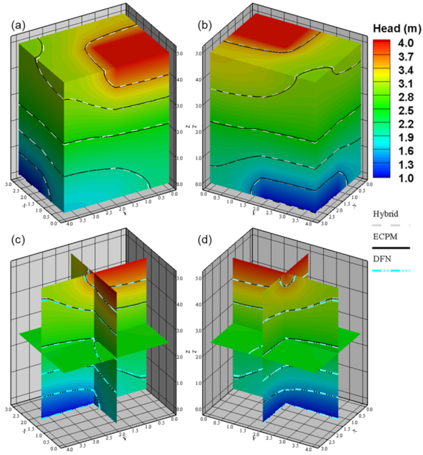
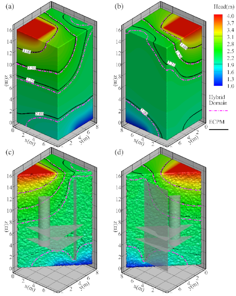
4.1. Flow Simulations Based on Different Models

Figure 7 shows the steady-state groundwater flow fields for Case I. Figure 7a,b compare results obtained from the HD and ECPM models, while Figure 7c,d present the head distributions only on the fractures. The results have shown the consistent solutions obtained from three different models. Specifically, the developed HD model enables the simulations of flow in fractures and rock matrix, which shows the advantage of the system of equations to be solved simultaneously. The concept proposed in the HD model can accurately capture the behavior of flow interactions between fractures and matrix (Figure 7a,b) and in the fractures network (Figure 7c,d). There is a difference of four orders of magnitude in hydraulic conductivity between the fractures and rock matrix in this case. The results of the HD model agree well with those obtained from the ECPM model in the entire domain region and the DFN model in the fracture network.

Figure 8 presents the flow results based on the conditions specified in Case II. This study excluded the DFN model because the three fractures have no contact with the domain surfaces. The results in Figure 8 indicate that the solutions obtained from the HD model show slightly deviated from the ECPM model, especially near the corners away from the specified head boundary conditions. In general, the overall pattern of the flow was captured by the developed HD model (Figure 8a,b). The results in Figure 8c,d show different views of the head distribution profile in the simulation domain. The head along the profile has demonstrated the considerable influence of the fractures on the head variation. The fractures provide fast pathways and control the local flow patterns to change with the fracture locations. Such behavior is significantly influenced by the vertical fracture near the top and bottom boundaries (see Figure 8c,d).

4.2. Simulations of Advective Transport

Figure 9 shows the particle traces and the associated trace lengths in Case I for three different models. Figure 9a,b show the release locations and the particle traces for the ECPM model. The results for the DFN model are shown in Figure 9e,f, while Figure 9c,d,g,h show the release location and the particle traces for the developed HD model. For comparison purposes, the HD results in Figure 9g,h only show the particles released along the edges of the fractures. In Case I, particles were randomly released on the inlet area, i.e., the specified head on the top boundary. The fracture hydraulic conductivity is four orders of magnitudes higher than the rock matrix. Figure 9a,b show that most particles directly penetrate the F3 and move to the outlet area with relatively small trace lengths in the ECPM model. However, the developed HD model shows that the fast pathway in F3 has significantly controlled the local flow and forced the particles to move along the fracture. No particle trace is shown in the block below the F3 fracture (see Figure 9c,d). All the particles move along the F3 and then follow the flow of the F1 and F2. In the ECPM model, the behavior of particle movement shows that the characteristic of high velocity in F3 is weak because the conductivity values of the F3 are lumped with the rock matrix conductivity in the upscaled cells in the ECPM model. Therefore, the hydraulic conductivity of the cells intersected by F3 might be slightly higher than the rock matrix after the upscaling process. In the ECPM model, the cell sizes intersected by fractures should be smaller than the fracture aperture to resolve the detailed flow behavior. However, it is impractical to consider small cell sizes for large-scale and complex fractured rock systems.

Figure 9e,f show the release locations and traces of particles for the DFN model. The boundary condition in the DFN model limited the particles to release on the edges of the intersections between fractures and the domain surface. Note that the particles are restricted to moving in the fractures plates. In Figure 9g,h, the particle traces on the virtual fractures were extracted from the HD model for comparison purposes. There are special trace circulations obtained on the F3, which was recognized as the local flow effect. The local flow effect is a unique feature in the 3D DFN model because of the interplay between fracture geometry and boundary conditions for flow in the fracture plates [47]. The local flow effect has little influence on flow in a 3D DFN but may constitute a mechanism that contributions to the long breakthrough tails and retardation observed in transport. The results obtained from the developed HD model captured the behavior of the local flow effect. However, the local flow behavior is relatively small as compared with those obtained from the DFN model.

Table 2. The statistics of the collected particle trace lengths, travel times, and velocities for Cases I.

Parameters		ECPM	HD (Fractures and Matrix)	DFN	HD (Fractures Only)
Trace length	Mean (m)	5.61	6.38	5.51	5.38
	STD (m)	0.35	1.01	0.63	0.37
	CV	0.062	0.158	0.114	0.069
	Min. (m)	5.07	5.12	5.11	5.10
	Max. (m)	6.39	10.48	9.04	7.77
Travel time	Mean (s)	$4.0 \times {10}^8$	$2.1 \times {10}^8$	$3.2 \times {10}^6$	$3.9 \times {10}^6$
	STD (s)	$2.3 \times {10}^8$	$6.4 \times {10}^7$	$4.7 \times {10}^6$	$2.6 \times {10}^6$
	CV	0.58	0.30	1.47	0.67
	Min. (s)	$6.4 \times {10}^7$	$1.4 \times {10}^5$	$1.8 \times {10}^6$	$1.8 \times {10}^6$
	Max. (s)	$1.2 \times {10}^9$	$6.3 \times {10}^8$	$5.6 \times {10}^7$	$3.1 \times {10}^7$
Velocity	Mean (m/s)	$2.0 \times {10}^{-8}$	$1.5 \times {10}^{-7}$	$2.4 \times {10}^{-6}$	$6.5 \times {10}^{-6}$
	STD (m/s)	$1.4 \times {10}^{-8}$	$1.3 \times {10}^{-7}$	$6.2 \times {10}^{-7}$	$6.3 \times {10}^{-7}$
	CV	0.70	0.87	0.26	0.10
	Min. (m/s)	$5.1 \times {10}^{-9}$	$8.8 \times {10}^{-9}$	$2.0 \times {10}^{-7}$	$2.0 \times {10}^{-7}$
	Max. (m/s)	$8.0 \times {10}^{-7}$	$3.6 \times {10}^{-5}$	$2.8 \times {10}^{-6}$	$2.9 \times {10}^{-6}$

summarizes the advective transport based on particle tracking applied to different models for Case I. Note that the velocity of each particle could be calculated by the observed trace length and the travel time. In Table 2, the results show that the mean trace length and the standard deviation (STD) and the coefficient of variation (CV) of the HD model are 1.14 times and 2.91 times higher than that of the ECPM model. There is no considerable deviation on the minimum trace length, but the maximum trace length of the HD model is 1.64 times higher than that of the ECPM model. The result indicates that most particles travel longer distances in the HD model because the fractures dominate the transport when the particles reach the fractures in the simulation domain. In this study, the STD of the trace length for the HD model is higher than that of the ECPM model. In general, the results show that the ECPM model underestimates the particle trace lengths and travel times in the case.

The particle movement statistics in Table 2 also show that the mean trace length and STD of the HD model are 0.98 and 0.59 times less than those of the DFN model. The minimal trace lengths for HD and DFN models are identical. However, the maximal trace length of the HD model is less than that of the DFN model. We found that the relatively significant local flow circulations in the DFN model lead to a longer trace length because of the particles that move in the horizontal fracture F3 [47]. Table 2 also shows the statistics of the traveling time for the released particles. Similar to the results of trace length, the HD model obtained lower mean and STD values of the particle travel time than those obtained from the ECPM model. Specifically, the minimum travel time of the HD model is two orders of magnitude less than that of the ECPM model, while the observed maximum travel time of the HD model is approximately half of the time obtained from the ECPM model. The results indicate that most particles in the HD model have fast traveling paths dominated by the fracture network. The short travel time is critical in conducting the safety assessment at a specific site. In general, the DFN model obtains relatively short travel times. The mean, minimum, and maximum travel times in the DFN model are generally one to two orders of magnitude smaller than those in the ECPM. However, the travel time variation (i.e., STD and CV) for the DFN model is relatively small compared with the results obtained from the HD and the ECPM models. This result is reasonable because the DFN model has constrained the particles to transport in the fracture network. Table 2 shows that the travel time statistics for the HD model vary between the results obtained from the ECPM and DFN models.

The results in Table 2 also show that the mean velocity of the HD model is 7.62 times higher than that of the ECPM model. In addition, the STD of the HD model is 9.62 times higher than that of the ECPM model. Note that the velocity calculation is based on the trace length and the travel time for a specific particle. The minimum velocity for the ECPM and HD models are in the same order. However, the maximum velocity of the HD model is considerably higher than that of the ECPM model because the particles in the HD model might move in the fractures. For the results obtained from the fracture-based DFN model, the HD model could reproduce well the overall behavior of the advective transport in fractures. The HD model enables the particles to move in fractures and the rock matrix with the feature of interactions between fractures and the rock matrix. We had discussed the computational issues for different approaches. The ECPM model requires the cell sizes to be small to resolve the detailed flow dynamics near fractures. The DFN ignores the influence of the rock matrix, which might partially decrease the velocity of advective transport. In this study, the developed HD model considers the virtual fractures embedded on the element face could be a feasible approach for problems with practical scales and complexity.

In Case II, the objective is to evaluate the influence of the DH added in the simulation domain. Figure 10 shows the released location and the particle traces for the ECPM and HD model.

Table 3. The results of the particle tracking simulation for Cases II.

Parameters	ECPM Model	HD Model
Start location (x, y, z) (m)	2.4375, 3.6875, 7.0625	3.390, 3.573, 5.000
End location (x, y, z) (m)	4.830, 4.147, 0.125	4.995, 4.114, 0.000
Velocity at the start location (m/s)	$1.31 \times {10}^{-10}$	$6.25 \times {10}^{-9}$

lists the detailed information for the results of particle tracking simulation for a specified release point in Case II. Note that the particle release point is the highest velocity based on the flow simulations obtained from the HD and ECPM models. Previous investigations had shown that the highest velocity was usually obtained along the intersections between the DH and fractures. In Case II, we had assigned a relatively large fracture aperture of 0.1 m. The large fracture aperture could reduce the number of cells for the ECPM model to capture the flow and transport influenced by the fracture geometries. However, this large fracture aperture might create differences in the highest velocities obtained from the ECPM and HD models. The location of a cell center in the ECPM model might not be consistent with the virtual fracture assigned on the element face.

In most practical problems, the highest velocity is the critical parameter for safety assessment in the near field of a disposal facility. The velocity is one of the parameters for calculating the buffer erosion and canister corrosion rate inside the deposition hole. The highest velocity location is also the point for releasing the containment in most practical problems [5]. Therefore, the value and location of the highest velocity are essential for the corresponding safety assessment of the disposal facility. The highest velocity location in the ECPM model is (2.4375 m, 3.6875 m, 7.0625 m) in Figure 10a,b, while the highest velocity location in the HD model is (3.390 m, 3.573 m, 5.000 m) in Figure 10c,d. In addition, the highest velocity value of the HD model is 47.88 times higher than that of the ECPM model. In this study, the ECPM and HD models obtain similar head distribution for Case II. However, the detected highest velocity locations in the two models are considerably different (see Table 3). The differences in the detected locations reveal two important technical issues, including (1) The different grid or mesh generations and hydraulic property fields are critical in influencing the location of the highest velocity on the intersection between a fracture and the DH, and (2) The z coordinate of the highest velocity location of the HD model is 5 m which is exactly the z coordinate of the fracture F5, while the location of ECPM model is at the center of a grid, which is 7.0625 m in this case based on the applied computational grids. In this study, the developed HD model considers the intersection as the inner boundary for mesh generation. The precise location of the highest velocity can be identified based on the solution at the node on the intersection.

This study further evaluated the uncertainty introduced by the fracture and DH intersections introduced in Case II. There were 48 particles released on the two intersections cut by fractures F4 and F5 (see Figure 10). Figure 11 shows the particle traces of the 48 released particles, and

Table 4. The statistics of the particle trackings for Cases II.

Parameters		ECPM Model	HD Model
Trace length	Mean (m)	10.69	9.07
	STD (m)	3.16	2.74
	CV	0.296	0.302
	Min. (m)	7.25	5.85
	Max. (m)	15.70	15.10
Travel time	Mean (s)	$9.70 \times {10}^9$	$4.25 \times {10}^9$
	STD (s)	$2.40 \times {10}^9$	$1.05 \times {10}^9$
	CV	0.247	0.247
	Min. (s)	$6.50 \times {10}^9$	$2.69 \times {10}^9$
	Max. (s)	$1.55 \times {10}^{10}$	$7.10 \times {10}^9$
Velocity	Mean (m/s)	$1.09 \times {10}^{-9}$	$2.18 \times {10}^{-9}$
	STD (m/s)	$1.56 \times {10}^{-10}$	$1.10 \times {10}^{-9}$
	CV	0.143	0.505
	Min. (s)	$8.31 \times {10}^{-10}$	$1.15 \times {10}^{-9}$
	Max. (s)	$1.37 \times {10}^{-9}$	$4.33 \times {10}^{-9}$

lists the statistics based on the collected particle traces and the travel times. The results in Figure 11a show that the particle traces in the ECPM model are similar, and the trace lines are uniformly distributed on the fracture surfaces. In the ECPM model, the pattern of the particle traces could capture well the two horizontal fracture geometry (see Figure 11a). Figure 11b shows the pattern of the particle traces in the HD model. The result demonstrates that the particle traces have been constrained in the narrow areas on the two fractures. Parts of the particles released from the intersection between F4 and DH migrate directly along the fracture F6 and then migrate to the rock matrix and reach the outlet boundary. A small portion of the particles might move along the F5 and then follow the particle traces starting from the intersection between DH and the fracture F5. The results present the significant difference between the ECPM and the HD models for the local flow behavior near the DH and fractures. The evaluations of the particle trace and traveling time can vary considerably if the release locations of the particles are different.

The statistics for the advection transport are summarized in Table 4. In general, the particle travel times obtained from the HD model are relatively small, leading to a relatively high transport velocity (Table 4). The mean velocity of the HD model could be two times higher than that in the ECPM model. Table 4 also shows that the HD model obtains relatively low STD values for the trace lengths and travel times but obtains high variation in transport velocity. Note that the HD model has considered virtual fractures in the simulation procedures. The particle release locations are precisely defined in the HD model. The fractures in the HD model act as a high-velocity pathway for groundwater flow. The particle migrations could be in fractures or rock matrices, depending on the local flow dynamics. For most practical problems, capturing the complex flow dynamics near DHs and fractures is essential for accurate evaluations of the large-scale and long-term transport processes.

5. Conclusions

This study has presented the concept of the HD approach for the simulation of advective transport in fractured rocks. Specifically, the developed HD model uses the 2D triangular mesh for fractures and tetrahedral mesh for the 3D rock matrix in a simulation domain and allows the system of equations to be solved simultaneously. The study employed two synthetic cases to assess the developed HD model. Solutions of flow and advective transport were compared with those obtained from the DFN model and ECPM model. In this study, the advective transport was conducted based on the particle tracking algorithm.

The simulation results show that the HD model is flexible in considering the concepts of DFN, ECPM, or both. Based on the test cases, the flow fields obtained from the HD model agree well with those obtained from the ECPM and DFN models. However, the local flow dynamics led to significant variations in the advective transport. Fractures in the simulation domain play an important role in controlling the local flow patterns. In addition, the released particle locations could also influence the particle traces and the travel times. The ECPM model might need fine grids to resolve the interaction dynamics between the fractures and rock matrix. The DFN model focuses on the fractures only and has the limited feature to account for the interaction between fractures and rock matrix. The local flow circulations are the special characteristic obtained from the DFN and the developed HD model.

The transport statistics relied on collecting the particle traces and travel times obtained from different models. The results in Case I indicated that the HD and DFN models obtained similar particle traces and travel times because the particles migrations have been restricted in the fractures. The particle released in the matrix and fractures might obtain different results from the ECPM and HD models. For the case with the particle release in the matrix (i.e., Case I), the HD model considered the detailed fracture flow and obtained a longer mean trace length than that obtained from the ECPM model. In Case II, the particles were released on the intersections between the DH and fractures. The HD model obtained a relatively small mean trace length and travel time. The identified highest velocity in the HD model is significantly greater than that in the ECPM model. The results have shown the feasibility of the HD model for accurate simulations of flow and advective transport in complex fractured rock systems.

References

1. Dershowitz, W.; Ambrose, R.; Lim, D.H.; Cottrell, M. Hydraulic Fracture and Natural Fracture Simulation for Improved Shale Gas Development. In Proceedings of the AAPG Annual Convention and Exhibition, Houston, TX, USA, 10–13 April 2011. Search and Discovery Article #40797. [Google Scholar]
2. Yan, B.; Mi, L.; Wang, Y.; Tang, H.; An, C.; Killough, J.E. Multi-porosity multi-physics compositional simulation for gas storage and transport in highly heterogeneous shales. J. Pet. Sci. Eng. 2018, 160, 498–509. [Google Scholar] [CrossRef]
3. Wang, H.Y. Discrete fracture networks modeling of shale gas production and revisit rate transient analysis in heterogeneous fractured reservoirs. J. Pet. Sci. Eng. 2018, 169, 796–812. [Google Scholar] [CrossRef]
4. AbuAisha, M.; Loret, B.; Eaton, D. Enhanced Geothermal Systems (EGS): Hydraulic fracturing in a thermo-poroelastic framework. J. Pet. Sci. Eng. 2016, 146, 1179–1191. [Google Scholar] [CrossRef]
5. Svensk Kärnbränslehantering AB; POSIVA Oy. Safety Functions, Performance Targets and Technical Design Requirements for a KBS-3V Repository, Conclusion and Recommendations from a Joint SKB and Posiva Working Group; Posiva SKB Report, 01; Svensk Kärnbränslehantering AB: Stockholm, Sweden; POSIVA Oy: Eurajoki, Finland, 2017. [Google Scholar]
6. Joyce, S.; Simpson, T.; Hartley, L.; Applegate, D.; Hoek, J.; Jackson, P.; Swan, D. Groundwater Flow Modelling of Periods with Temperate Climate Conditions—Forsmark; R-09-20; Svensk Kärnbränslehantering AB: Stockholm, Sweden, 2010. [Google Scholar]
7. Hyman, J.D.; Gable, C.W.; Painter, S.L.; Makedonska, N. Conforming delaunay triangulation of stochastically generated three dimensional discrete fracture networks: A feature rejection algorithm for meshing strategy. J. Sci. Comput. 2014, 36, A1871–A1894. [Google Scholar] [CrossRef]
8. Hyman, J.D.; Karra, S.; Makedonska, N.; Gable, C.W.; Painter, S.L.; Viswanathan, H.S. dfnWorks: A discrete fracture network framework for modeling subsurface flow and transport. Comput. Geosci. 2015, 84, 10–19. [Google Scholar] [CrossRef] [Green Version]
9. Kalbacher, T.; Wang, W.; McDermott, C.; Kolditz, O.; Taniguchi, T. Development and application of a CAD interface for fractured rock. Eng. Geol. 2005, 47, 1017–1027. [Google Scholar] [CrossRef]
10. Makedonska, N.; Painter, S.; Bui, Q.; Gable, C.; Karra, S. Particle tracking approach for transport in three-dimensional discrete fracture networks. Comput. Geosci. 2015, 19, 1123–1137. [Google Scholar] [CrossRef]
11. Zhang, Q.H. Finite element generation of arbitrary 3-D fracture networks for flow analysis in complicated discrete fracture networks. J. Hydrol. 2015, 529, 890–908. [Google Scholar] [CrossRef]
12. Chen, R.H.; Lee, C.H.; Chen, C.S. Evaluation of transport of radioactive contaminant in fractured rock. Environ. Geol. 2001, 41, 440–450. [Google Scholar] [CrossRef]
13. Jing, L. A review of techniques, advances and outstanding issues in numerical modelling for rock mechanics and rock engineering. Int. J. Min. Reclam. Environ. 2003, 40, 283–353. [Google Scholar] [CrossRef]
14. Rutqvist, J.; Leung, C.; Hoch, A.; Wang, Y.; Wang, Z. Linked multicontinuum and crack tensor approach for modeling of coupled geomechanics, fluid flow and transport in fractured rock. J. Rock Mech. Geotech. Eng. 2013, 5, 18–31. [Google Scholar] [CrossRef] [Green Version]
15. Vu, P.T.; Ni, C.-F.; Li, W.-C.; Lee, I.-H.; Lin, C.-P. Particle-Based Workflow for Modeling Uncertainty of Reactive Transport in 3D Discrete Fracture Networks. Water 2019, 11, 2502. [Google Scholar] [CrossRef] [Green Version]
16. Berrone, S.; Pieraccini, S.; Scialò, S. A PDE-constrained optimization formulation for discrete fracture network flows. J. Sci. Comput. 2013, 35, B487–B510. [Google Scholar] [CrossRef]
17. Berrone, S.; Pieraccini, S.; Scialò, S. An optimization approach for large scale simulations of discrete fracture network flows. J. Comput. Phys. 2014, 256, 838–853. [Google Scholar] [CrossRef] [Green Version]
18. Neuman, S. Trends, prospects and challenges in quantifying flow and transport through fractured rocks. Hydrogeol. J. 2005, 13, 124–147. [Google Scholar] [CrossRef]
19. Peratta, A.; Popov, V. A new scheme for numerical modelling of flow and transport processes in 3D fractured porous media. Adv. Water Resour. 2006, 29, 42–61. [Google Scholar] [CrossRef]
20. Maryška, J.; Severýn, O.; Vohralík, M. Numerical simulation of fracture flow with a mixed-hybrid FEM stochastic discrete fracture network model. Comput. Geosci. 2005, 8, 217–234. [Google Scholar] [CrossRef]
21. Berre, I.; Boon, W.; Flemisch, B.; Fumagalli, A.; Glaser, D.; Keilegavlen, E.; Scotti, A.; Stefansson, I.; Tatomir, A. Call for participation: Verification benchmarks for single-phase flow in three-dimensional fractured porous media. Math. NA 2018, 1809, 1–20. [Google Scholar]
22. Berre, I.; Boon, W.M.; Flemisch, B.; Fumagalli, A.; Gläser, D.; Keilegavlen, E.; Scotti, A.; Stefansson, I.; Tatomir, A.; Brenner, K.; et al. Verification benchmarks for single-phase flow in three-dimensional fractured porous media. Adv. Water Resour. 2021, 147, 103759. [Google Scholar] [CrossRef]
23. Li, S.C.; Xu, Z.H.; Ma, G.W.; Yang, W.M. An adaptive mesh refinement method for a medium with discrete fracture network: The enriched Persson’s method. Finite Elem. Anal. Des. 2014, 86, 41–50. [Google Scholar] [CrossRef]
24. Wang, L.; Cardenas, M.B. An efficient quasi-3D particle tracking-based approach for transport through fractures with application to dynamic dispersion calculation. J. Contam. Hydrol. 2015, 179, 47–54. [Google Scholar] [CrossRef] [PubMed] [Green Version]
25. Golder. Available online: https://www.golder.com/fracman/ (accessed on 3 October 2021).
26. Golder. Fracman7 Interactive Discrete Feature Data Analysis, Geometric Modeling and Exploration Simulation; User Documenation; Golder Associates: Seattle, WA, USA, 2018; pp. 1–567. [Google Scholar]
27. Svensson, U. A continuum representation of fracture networks. Part I: Method and basic test cases. J. Hydrol. 2001, 250, 170–186. [Google Scholar] [CrossRef]
28. Svensson, U. A continuum representation of fracture networks. Part II: Application to the Äspö Hard Rock laboratory. J. Hydrol. 2001, 250, 187–205. [Google Scholar] [CrossRef]
29. Svensson, U.; Ferry, M. DarcyTools: A computer code for hydrogeological analysis of nuclear waste repositories in fractured rock. J. Appl. Math. Phys. 2014, 2, 365–383. [Google Scholar] [CrossRef]
30. Kwicklis, E.M.; Healy, R.W. Numerical investigation of steady liquid water flow in a variably saturated fracture network. Water Resour. Res. 1993, 29, 4091–4102. [Google Scholar] [CrossRef]
31. Liu, H.H.; Bodvarsson, G.S.; Finsterle, S. A note on unsaturated flow in two-dimensional fracture networks. Water Resour. Res. 2002, 38, 15-1–15-9. [Google Scholar] [CrossRef]
32. Pruess, K.; Tsang, Y.W. On two-phase relative permeability and capillary pressure of rough-walled rock fractures. Water Resour. Res. 1990, 26, 1915–1926. [Google Scholar] [CrossRef] [Green Version]
33. Lee, I.H.; Ni, C.F. Fracture-based modeling of complex flow and CO2 migration in three-dimensional fractured rocks. Comput. Geosci. 2011, 81, 2270–2281. [Google Scholar] [CrossRef]
34. Lee, I.H.; Ni, C.F.; Lin, F.P.; Lin, C.P.; Ke, C.C. Stochastic modeling of flow and conservative transport in three-dimensional discrete fracture networks. Hydrol. Earth Syst. Sci. 2019, 23, 19–34. [Google Scholar] [CrossRef] [Green Version]
35. Mustapha, H.; Dimitrakopoulos, R.; Graf, T.; Firoozabadi, A. An efficient method for discretizing 3D fractured mediafor subsurface flow and transport simulations. Int. J. Numer. Meth. Fluids 2011, 81, 651–670. [Google Scholar] [CrossRef]
36. Du, Q.; Wang, D. Recent progress in robust and quality Delaunay mesh generation. J. Comput. Appl. Math. Fluids 2006, 195, 8–23. [Google Scholar] [CrossRef] [Green Version]
37. Ghadyani, H.; Sullivan, J.; Wu, Z. Boundary recovery for delaunay tetrahedral meshes using local topological transformations. Finite Elem. Anal. Des. 2010, 46, 74–83. [Google Scholar] [CrossRef] [Green Version]
38. Sun, S.; Sui, J.; Chen, B.; Yuan, M. An efficient mesh generation method for fractured network system based on dynamic grid deformation. Math. Probl. Eng. 2013, 2013, 834908. [Google Scholar] [CrossRef]
39. Zhang, Y.; Bajaj, C.; Sohn, B.S. 3D finite element meshing from imaging data. Comput. Methods Appl. Mech. Eng. 2005, 194, 5083–5106. [Google Scholar] [CrossRef] [Green Version]
40. Hyman, J.D.; Painter, S.L.; Viswanathan, H.; Makedonska, N.; Karra, S. Influence of injection mode on transport properties in kilometer-scale three-dimensional discrete fracture networks. Water Resour. Res. 2015, 51, 7289–7308. [Google Scholar] [CrossRef]
41. Painter, S.; Cvetkovic, V.; Mancillas, J.; Pensado, O. Time domain particle tracking methods for simulating transport with retention and first-order transformation. Water Resour. Res. 2008, 44, 1–11. [Google Scholar] [CrossRef]
42. Kensler, A.; Shirley, P. Optimizing Ray-Triangle Intersection via Automated Search. In Proceedings of the IEEE Symposium on Interactive Ray Tracing, Salt Lake City, UT, USA, 18–20 September 2006. [Google Scholar]
43. Fougerolle, Y.D.; Lanquetin, S.; Neveu, M.; Lauthelier, T. A Geometric Algorithm for Ray/Bézier Surfaces Intersection Using Quasi-Interpolating Control Net. In Proceedings of the IEEE International Conference on Signal Image Technology and Internet Based Systems, Bali, Indonesia, 30 November–3 December 2008. [Google Scholar]
44. Maria, M.; Horna, S.; Aveneau, L. Efficient Ray Traversal of Constrained Delaunay Tetrahedralization. In Proceedings of the 12th International Joint Conference on Computer Vision, Imaging and Computer Graphics Theory and Applications (VISIGRAPP 2017), Porto, Portugal, 27 February–1 March 2017. [Google Scholar]
45. Svensk Kärnbränslehantering AB. Buffer, Backfill and Closure Process Report for the Safety Assessment SR-Site; TR-10-47; Svensk Kärnbränslehantering AB: Stockholm, Sweden, 2010. [Google Scholar]
46. Svensk Kärnbränslehantering AB. Radionuclide Transport Report for the Safety Assessment SR-Site; TR-10-50; Svensk Kärnbränslehantering AB: Stockholm, Sweden, 2010. [Google Scholar]
47. Park, Y.L.; Lee, K.K.; Kosakowski, G.; Berkowitz, B. Transport behavior in three-dimensional fracture intersections. Water Resour. Res. 2003, 39, 1215. [Google Scholar] [CrossRef] [Green Version]
Figure 1. An example that shows two fractures and the corresponding 2D and 3D meshes for the proposed HD model. (a) The geometry of the fractures inside the modeling domain; (b) The generated triangular meshes for the fractures near the intersection; (c) The exterior view of the generated meshes for the simulation domain; (d) A profile view shows the interior of the generated meshes for the simulation domain.
Applsci 11 10792 g001
Figure 2. The demonstration of the particle tracking algorithm for a particle trace and the associated element along the trace line: (a) The overall particle moving paths starting from the point “Start” and end with the point “End”; (b) The local enlargement for the selected elements (marked with grey color in (a) and the particle trace outside the selected elements; (c) The drawing of local enlargement that shows the particle trace and the associated intersection point on the element face.
Applsci 11 10792 g002
Figure 3. The main steps involved in the workflow to model flow and advective transport in fractured rocks.
Applsci 11 10792 g003
Figure 4. The conceptual model of the benchmark cases in this study: (a) Case I includes three orthogonal fractures (F1 to F3) in the simulation domain; (b) Case II includes three fractures (F4 to F6) and a deposition hole (DH) in the fractured rock. Note that the contours show the elevation of the fractures.
Applsci 11 10792 g004
Figure 5. The computational mesh of the test Case I for the HD model: (a) The generated mesh for the fractures (in blue color) and the associated matrix (in black color); (b) The inner view of the mesh for the fractures (in blue color) and matrix (in black color); (c) The mesh for fractures; (d) The close view of the generated nodes and elements for the connections of fractures (in blue color) and matrix (in black color) in the HD model.
Applsci 11 10792 g005
Figure 6. The computational mesh of the test Case II for the HD model: (a) The geometry of fractures (in blue color) and DH object (in black color); (b) The zoom-in view of the mesh generated for connecting the matrix and the DH object; (c) The close view of the generated nodes and elements for the connections of fractures, matrix, and DH object. Note that parts of the meshes in the figures are blanked for presentation purposes.
Applsci 11 10792 g006
Figure 7. The steady-state head distributions obtained from the HD, DFN, and ECPM models for Case I: (a,b) The solutions for the HD and ECPM models; (c,d) The heads obtained from the HD and DFN models for the fractures.
Applsci 11 10792 g007
Figure 8. The head distributions obtained from the HD and ECPM models for Case II: (a,b) The head solutions on the surfaces of the simulation domain; (c,d) The different angle views of heads for the specified profile.
Applsci 11 10792 g008
Figure 9. The particle traces and lengths obtained from the ECPM, DFN, and HD models for Case I: (a,b) The particle traces for the ECPM model; (c,d) The particle traces for the HD model; (e,f) The particle traces for the DFN model; and (g,h) The particle trace along the fractures for the HD model.
Applsci 11 10792 g009
Figure 10. The particle release location and the particle trace for the ECPM and HD models in Case II. (a,b) The start location and particle trace for the ECPM model; (c,d) The start location and particle traces for the HD model.
Applsci 11 10792 g010
Figure 11. The results of particle traces based on the 48 particles released on the two intersections between DH and fractures F4 and F5: (a) The trace lines for the ECPM model, and (b) The trace lines for the developed HD model.
Applsci 11 10792 g011