Article

Neural Identification of a Temperature Field in the Storing Phase of Thermal Energy in Rock Bed Thermal Storage

Faculty of Biosystems Engineering, Poznań University of Life Sciences, 60-625 Poznań, Poland
*
Author to whom correspondence should be addressed.
Appl. Sci. 2021, 11(22), 10711; https://doi.org/10.3390/app112210711
Submission received: 3 October 2021 / Revised: 7 November 2021 / Accepted: 9 November 2021 / Published: 13 November 2021

Abstract

:
Thermal energy stored within a rock bed thermal storage system, which is mostly used in agriculture, can be identified during the storage phase using mathematical models based on heat transfer, which concerns batteries running in a vertical setting. However, this requires the conversion of differential equations into algebraic equations, as well as knowledge about the initial and boundary conditions. Furthermore, a lack of information or incomplete information about the initial conditions makes it difficult or impossible to evaluate the volume of stored energy, or can cause significant errors during evaluation. Such situations occur in systems equipped with a rock battery, in which solar collectors act as source of energy. Considering the above, as well as the lack of a model for batteries in a vertical setting, we identified the need for research into the storage phase of rock bed thermal storage systems, working in a horizontal setting, and generating MLP-type neural models. Among these models, MLP 4-7-1 turned out to be the best both in terms of the values of regression statistics and possibilities of generalization. According to the authors, artificial neural models depicting temperature changeability in storage phase will be helpful in the development of a new methodology that can predict the heat volume in rock bed thermal storage systems.

1. Introduction

The amount of energy in a power system that is stored in a rock bed is one of several possible, mostly unconventional, sources of energy, and is not particularly hard to identify. In this case, automatic regulation systems were applied, which disabled the flow of the medium through the deposit when the output temperature fell below the required value. However, with a limited number of unconventional sources and a sensible thermal energy management system, information about the quantity of heat stored in any rock bed would be welcome [1,2,3]. This Such cases occur in agriculture, where solar panels (characterized by a variable amount of energy supply) are used as one of the energy sources [4,5]. The effective and economically viable use of such energy sources, for example, to dry crops or heat greenhouses, requires not only the use of heat accumulators with a simple structure, such as rock bed storage, but also a method for assessing the amount of thermal energy they accumulate, which would be simple and acceptable in practice.
In order to achieve this goal, the following mathematical models of heat flow should be used [4,5,6,7]. Although the storage phase is the most difficult phase to model, we currently have mathematical models that describe this stage of a rock bed heat accumulator’s operation [8,9].
A comprehensive description of heat flow during the stagnation phase of rock bed thermal storage, presented in the form of deductive mathematical models, can be found in the work of Stamps and his research team [10,11]. The authors proposed two models that differed as their assumed simplifications and considered accumulators worked in a vertical setting. In addition to the single temperature model (based on only one field of temperatures, assuming an identical rock bed and air temperature), we shall focus on the two-temperature model, as it bears more similarity to the empirical system. This model consists of several equations of flow continuity and momentum, and two equations of energy balance for the air and the deposit, as appropriate (Equations (1)–(4)).
A flow continuity equation:
· U = 0
where U—averaged air velocity in an elementary volume [m·s−1].
A momentum equation:
a μ ψ U + b ρ f ψ 2 | U | U = p T + ρ f o β ( T f T o ) g k
where:
  • α—Darcy’s constant [m−2];
  • μ—dynamic viscosity [kg·(m·s)−1];
  • ψ—porosity;
  • ρf—fluid density [kg·m−3];
  • ρfo—fluid density at the reference temperature [kg·m−3];
  • b—Forchheimer’s constant [m−1];
  • pT—dynamic pressure [Pa];
  • β—volumetric temperature expansion coefficient [K−1];
  • Tf—air temperature [K];
  • To—reference temperature [K];
  • g—acceleration due to gravity [m·s−2];
  • k—vertical unit vector.
The equation for fluid energy balance:
( ρ f c f p ) ψ T f t + ( ρ f c f p ) ψ U · T f = k f 2 T f + h A s f ( T s T f )
where:
  • Asf—interface surface [m2];
  • cfp—fluid specific heat [J·(kg·K)−1];
  • kf—effective thermal conductivity of fluid [W·(m·K)−1];
  • h—convective heat transfer coefficient [W·(m2·K)−1];
  • Ts—deposit temperature [K];
  • t—time [s];
  • ∀—volume deposit [m3].
Rock bed energy balance equation:
( ρ s c s p ) ( 1 ψ ) T s t = k s 2 T s + h A s f ( T f T s )
where:
  • csp—rock-bed-specific heat [J·(kg·K)−1];
  • ks—effective thermal conductivity of rock bed [W·(m·K)−1];
  • ρs—rock bed density [kg·m−3].
The solution to the above equations proposed by Stamps’ research team [8,11] required them to be converted into a non-dimensional form, using vector potential and the simultaneous formulation of the initial and boundary conditions. Next, the resulting mathematical structures formed the basis for using numerical methods to obtain the solution. Thus the fields of discrete temperature obtained enabled the identification of the energy accumulated in the deposit. It is possible to use this procedure in a real situation, assuming we have an accumulator working in the vertical setting, an IT system to map the model, and the initial and boundary conditions. As mentioned before, the problem in evaluating the amount of thermal energy that was accumulated may be the unavailability and ignorance of the initial conditions based on the temperature distribution in the deposit at the beginning of the storage process.
The available models are converted into algebraic equations, regarding layers of rock in a vertical system/layout. Having mathematical models to identify the temperature fields is necessary to determine the amount of energy stored within the deposits; however, first one must determine the initial input and boundary conditions [9,10]. In practice, due to economic reasons, we lacked all the information on the conditions, and the data on the initial conditions were particularly sparse. This was a concern for almost all situations, especially the one in which a solar collector was used as a source of thermal energy. The stochastic character of this source, combined with the heterogenous flow of air during the loading phase preceded by the phase of battery stagnation, hindered the determination of the initial conditions, which are necessary in order to evaluate the volume of currently collected thermal energy within the battery using the available mathematical models. From a practical perspective, it is considered appropriate to find a limitation with regard to the economical points of temperature measurement within the rock deposit, the readings of which would allow one to determine the volume of thermal energy stored there. Knowing the initial conditions would then no longer be necessary. This mainly concerns situations that involve the battery being charged from a thermal source of stochastic character. The aim of the study is to answer the following question: To what extent can they be helpful in building up the methods of neural modeling? The answer to the above question must be preceded by a statement that confirms the possibility of designing neural models and describes the phase of storing thermal energy. This specific problem is the subject matter of this article. Having neural models depicting changeable temperatures in field, and in the function of time and space, allows us to identify thermal energy currently collected in a given deposit. This, in turn, will allow us to search for the smallest possible point or points of temperature measurement (considering economic reasons), which will allow us to identify thermal energy stored in rock deposits at any moment, independently of the initial conditions and with a broader knowledge of the boundary conditions [12,13].

2. Materials and Methods

2.1. Storage Phase of the Rock Bed Thermal Storage

An alternative to the classical description and an analysis of empirical systems was found in modern methods, such as artificial neural modeling [14,15]. Artificial neural networks (ANN) are a branch of science that has developed intensively [16], and the main advantage of the neural models has been their ability to generalize the knowledge acquired through training. The fields of application in which neural models have proved to be effective include forecasting, recognition or classification and diagnostics, for example, in agriculture [17,18]. As opposed to the traditional information-processing methods offered by computers, which execute a series of pre-developed algorithms, the basis for the development and subsequent operation of neural networks has been the use of what are known as training algorithms. This use of advanced optimization training algorithms has allowed an appropriate neural network structure to be designed, and a selection of the parameters set to suit the specific problem that requires solving [19]. Among these problems, others have emerged that relate to the use of thermal energy supplied from unconventional energy sources in agriculture [20,21,22,23]. Generally, the techniques of neural modeling in this area are often used to describe the temperature distribution [24,25].
An effective way of identifying the amount of thermal energy accumulated in a rock bed could be based on artificial neural networks as predictive instruments. However, this requires prior evaluation of the usefulness of the neural models for describing the thermal energy storage phase of the thermal accumulator. Many authors have made successful attempts to develop neural models to describe the charging phase [26], which have proved useful, for example, in the process of identifying uneven air flows through the deposit. The basis for building the original neural models originated from the results of a natural experiment, in which the subject was a rock bed thermal storage system working in a horizontal setting and designed to work with a solar collector. The work of the sun collector was steered with the heater, as illustrated in Figure 1. Broken granite stone with an average substitute diameter of 0.039 m, calculated on the basis of measurement of the volume of deposit elements, was used as a warehouse filling. Granite is characterized by relatively good heat properties such as thermal properties and specific heat. From an economic perspective, this material is highly recommended. The two remaining volumes were compensatory chambers. The simplified construction of the test stand, along with its simplified structure and layout of temperature sensors, is shown in Figure 1 and Figure 2. PT100 sensors that measured temperature with a measuring accuracy of 0.1 °C were arranged in three perpendicular dimensions. The temperature measurement was also used to determine the inequality of airflow during the charging stage. Heat processes in the battery were related as low-frequency variables. As such, temperatures were registered at 5 min intervals. Due to the characteristics of the battery filling, this was included in the short-term storage group and was insulated with a layer of polystyrene with a thickness of 0.06 m. The total volume of the battery was 3 m3, of which 83% consisted of a bed and the remainder an equalizing chamber that improved the uniformity of air flow during the charging and discharging phases. The duration of the thermal energy storage phase did not exceed 15 h. Subsequently, the temperatures recorded during the storage phase emerged as the essential source of data necessary to develop the neural models.

2.2. Neural Models of Temperature Distribution

The neural models for predicting the temperature recorded during the storage phase of the accumulator were developed in the Matlab environment, using the Neural Network Toolbox add-on. The network’s structures consist of an Multi-Layer Perceptron (MLP) [17,27,28,29,30] with 4 inputs, a diverse number of neurons in the hidden layer (5 or 10 neurons) and 1 neuron in the output layer.
The one-way multilayer networks of the multilayer perceptron type are among the most studied and most commonly used network topologies. ANN-type MLP represents the so-called parametric neural model class. For example, they are characterized by the fact that the number of neurons forming their structure is markedly lower than the learning file size. The defined input variables and output variable are shown in Table 1.
The collection of data necessary to develop the neural model was, by default, divided, in the ratio 2:1:1, into the following files: training, validation and testing. These files included, respectively: 1008, 504 and 504 cases. The testing file was not used in the network training process, as this was essential for the final evaluation of the neural model. A fragment of the training file (cases from 331 to 337) is shown in Table 2.
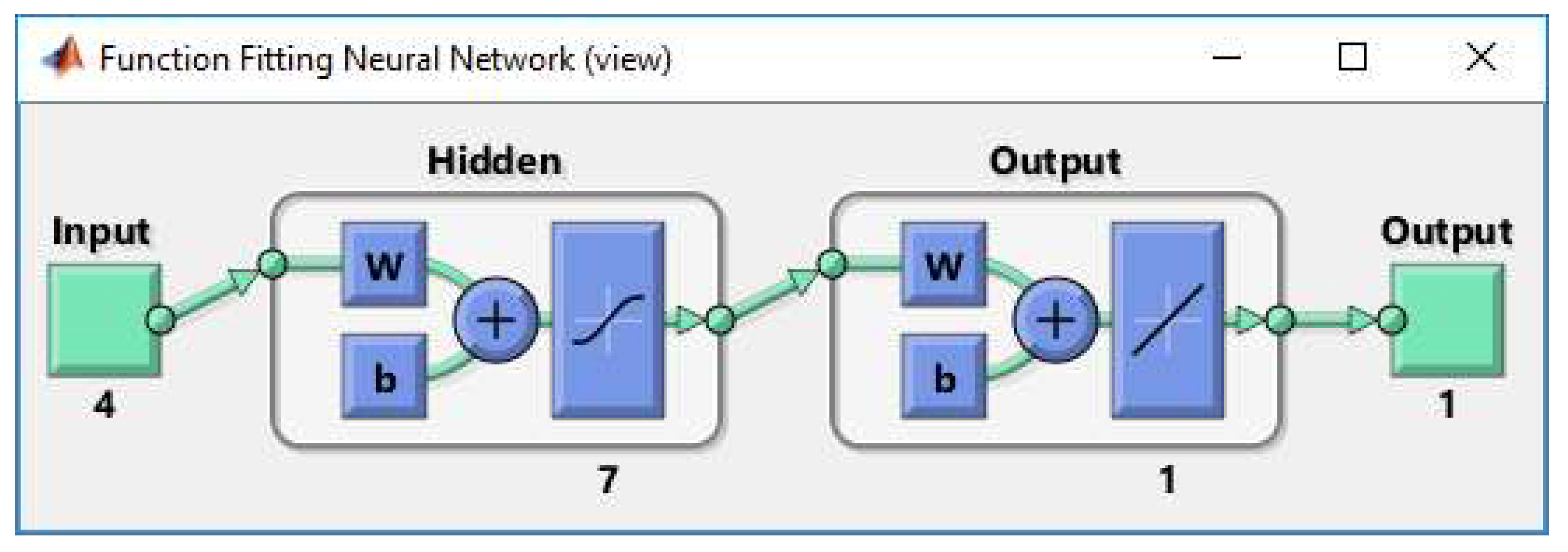
The developed ANNs were trained using an error back propagation algorithm (BP) with Bayesian regularisation. Mean Squared Error (MSE) was used as the error function. The neural networks generated were designated as MLP 4-5-1, MLP 4-7-1 and MLP 4-10-1. The sigmoid function was used as the activation function for the hidden layer neurons, and a linear function was used for the output layer neurons. The structure of the neural model MLP 4-7-1 is shown in Figure 3.
In the network training process in the Matlab environment, the following algorithm stoppage criteria were adopted:
  • Maximum training epochs (epochs parameter): 1500;
  • Maximum subsequent epochs, in which the error function value may deteriorate for the validation file (max_fail parameter): 100;
  • Minimum error function gradient (min_grad parameter): 1 × 10⁻⁷.

3. Results

The standard measure of quality for the generated neural model is the RMS error, which is defined as follows:
R M S = i = 1 n ( T m i T p i ) 2 n
where:
  • n—number of cases;
  • Tmi—measured values of temperature;
  • Tpi—values of temperature predicted with the use of the neural model.
The RMS error values for the MLP 4-5-1 neural model were:
  • 0.4324 for the training file;
  • 0.4462 for the validation file;
  • 0.4554 for the test file.
The RMS error values for the MLP 4-7-1 neural model were:
  • 0.2604 for the training file;
  • 0.2780 for the validation file;
  • 0.2809 for the test file.
The error values for the MLP 4-10-1 neural model were:
  • 0.1437 for the training file;
  • 0.1626 for the validation file;
  • 0.1578 for the test file.
The created MLP with 4-5-1, 4-7-1 and 4-10-1, respectively, were characterized by generally low error values with a falling tendency together with the increase in the number of neurons in the hidden layer. Complete and full statistics of regression for all created models are presented in Table 3. Having noticed the fact that the network with 10 neurons within the hidden layer showed a tendency to over-learn, a decision was made to use a model with an MLP 4-7-1 network in the process of modeling temperature layout in the rock regenerator. Notably, this model showed good generalization abilities/capabilities.
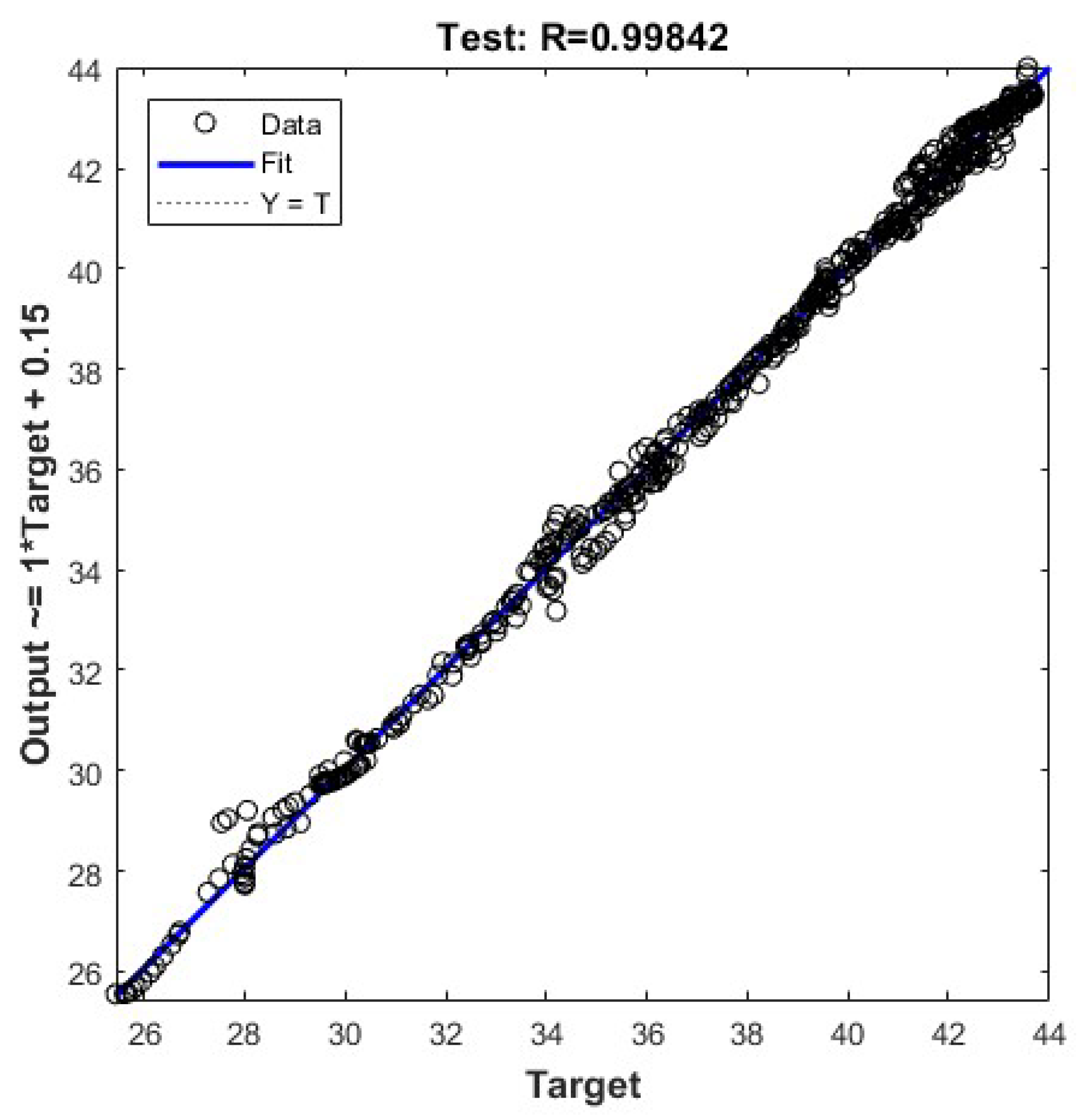
Figure 4 presents the information on the linear regression between the temperature values obtained using the MLP 4-7-1 model and the values of that parameter for the testing file. Information on the absolute error of temperature determination was also included in the form of a histogram (Figure 5). The regression coefficient for the model was 0.998. Thus, one may assert that the results of the temperature prediction as a function of position, and charging time obtained using the model that was generated, closely reflected the results of the natural experiment included in the testing file.
The high quality of the generated MLP 4-7-1 network as a prediction instrument was identified by the regression statistics presented in Table 3. The statistics included the following indicators:
  • Data Mean—the mean value of the output variable calculated based on the required values of this variable, collected in the training, validation or testing files, as appropriate. The regression statistics were determined independently for the training, validation and testing files.
  • Data S.D.—the standard deviation calculated for the required (as above) values of the output variable.
  • Error Mean—mean error (the modulus of difference between the required value and the obtained output value) for the output variable.
  • Error S.D.—standard deviation of errors for an output variable.
  • Abs Mean—mean absolute error (difference between the required value and the obtained output value) for the output variable.
  • S.D. Ratio—the ratio of standard deviations for the errors and for the data. This was the main quality coefficient of the regression model generated by the network.
  • Correlation—the standard Pearson R correlation coefficient for the values required and obtained at the output.
The two final indicators presented in Table 3, namely, the ratio of standard deviations and correlation, were essential for evaluating the predictive capacity of the developed neural network. The lower the ratio of the standard deviations (closer to zero) and the higher the correlation (closer to one), the better the network. Table 3 shows that the correlation was about 0.998, which was a close approximate for the files: training, validation and testing, although the ratio of the standard deviations for the errors and for the data was in the 0.05 range.
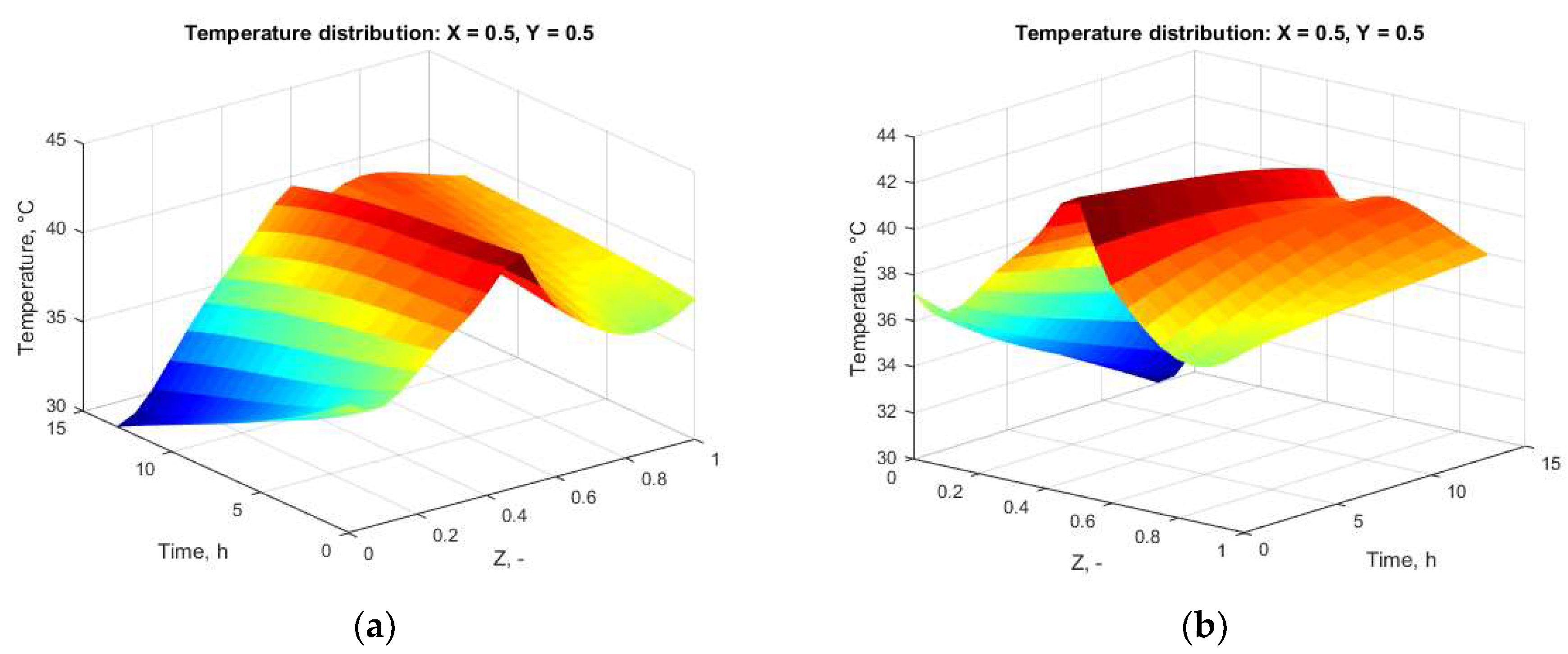
The indicative visualization of the neural network operations that were generated was a 2-dimensional function, referred to as the network response area. For variables Z and t (at the defined X = 0.5 and Y = 0.5), the response surface of the MLP 4-7-1 network is shown in Figure 6. Undoubtedly, the visualization of the temperature distribution in the rock bed heat storage during the stagnation phase, based on this neural model, more fully represented the heat flow caused mainly by free convection.
In the case of the generated surface, with all the assumed principles (at the defined X = 0.5 and Y = 0.5), by MLP 4-10-1 network, we can observe some disturbances in the layout, namely the occurrence of two temperature maximums at the end of the storage process (see Figure 7). Such a temperature layout has no physical grounds and was the reason this neural model was rejected. In the opinion of the authors, this was the effect of network’s over-learning.

4. Conclusions

Research into the storage phase of thermal energy in a rock bed thermal storage system working in a horizontal setting has provided the necessary date to generate an optimum MLP 4-7-1 neural model. The qualitative evaluation of the neural model as a tool for predicting the deposit temperature as a function of position and time has been successful. This has also been confirmed with diagrams, which depicted the moving of areas with the highest temperature to the top of the deposit along with the passing of time in storage, and was the result of natural convection. Out of three MLP models that were analyzed, the one that was characterized by the lowest error value and maintained generalization abilities/capabilities was a neural network with seven neurons in the hidden layer. The positive values of regression statistics proved the usefulness of neural modeling for the description of the deposit temperature field variation in the stagnation phase. They suggested the usefulness of further research aimed at using this tool in the process of developing a new method of identifying the amount of energy aggregated in rock bed thermal storage, and one that would be convenient and financially viable.
This new methodology depends on determining the position of point or points of temperature measurement with limited numbers within a deposit. Independent of the readings of the initial conditions, such temperature measurements would be sufficient to evaluate the amount of thermal energy stored in a horizontal rock deposit.

Author Contributions

Conceptualization, W.M., S.K. and K.K.; methodology, W.M. and S.K.; validation, S.K., K.K.; formal analysis, W.M. and K.K.; investigation, W.M.; resources, W.M.; writing—original draft preparation, W.M., K.K.; writing—review and editing, K.K.; visualization, W.M. and S.K.; supervision, W.M. All authors have read and agreed to the published version of the manuscript.

Funding

This research received no external funding.

Institutional Review Board Statement

Not applicable.

Informed Consent Statement

Not applicable.

Data Availability Statement

Not applicable.

Conflicts of Interest

The authors declare no conflict of interest.

References

  1. Ramadan, M.R.I.; El-Sebaii, A.A.; Aboul-Enein, S.; El-Bialy, E. Thermal performance of a packed bed double-pass solar air heater. Energy 2007, 32, 1524–1535. [Google Scholar] [CrossRef]
  2. Baghban, A.; Kahani, M.; Nazari, M.A.; Ahmadi, M.H.; Yan, W.H. Sensitivity analysis and application of machine learning methods to predict the heat transfer performance of CNT/water nanofluid flows through coils. Int. J. Heat Mass Transf. 2019, 128, 825–835. [Google Scholar] [CrossRef]
  3. Ahmadi, M.H.; Nazari, M.A.; Ghasempour, R.; Madah, H.; Shafii, M.B.; Ahmadi, M.A. Thermal conductivity ratio prediction of Al2O3/water nanofluid by applying connectionist methods. Colloids Surf. Physicochem. Eng. Asp. 2018, 541, 154–164. [Google Scholar] [CrossRef]
  4. Hänchen, M.; Brückner, S.; Steinfeld, A. High-temperature thermal storage using a packed bed of rocks—Heat transfer analysis and experimental validation. Appl. Therm. Eng. 2011, 31, 1798–1806. [Google Scholar] [CrossRef]
  5. Bindra, H.; Bueno, P.; Morris, J.F.; Shinnar, R. Thermal analysis and exergy evaluation of packed bed thermal storage systems. Appl. Therm. Eng. 2013, 52, 255–263. [Google Scholar] [CrossRef]
  6. N G Barton, “Simulations of air-blown thermal storage in a rock bed. Appl. Therm. Eng. 2013, 55, 43–50. [CrossRef]
  7. Sadeghzadeh, M.; Ahmadi, M.H.; Kahani, M.; Sakhaeinia, H.; Chaji, H.; Chen, L. Smart modeling by using artificial intelligent techniques on thermal performance of flat-plate solar collector using nanofluid. Energy Sci. Eng. 2019, 7, 1649–1658. [Google Scholar] [CrossRef]
  8. Stamps, D.W.; Clark, J.A. Thermal destratification in a cylindrical packed bed. Int. J. Heat Mass Transf. 1992, 35, 727–737. [Google Scholar] [CrossRef] [Green Version]
  9. Ahmadi, M.H.; Mohseni-Gharyehsafa, B.; Ghazvini, M.; Goodarzi, M.; Jilte, R.D.; Kumar, R. Comparing various machine learning approaches in modeling the dynamic viscosity of CuO/water nanofluid. J. Therm. Anal. Calorim. 2020, 139, 2585–2599. [Google Scholar] [CrossRef]
  10. Pintaldi, S.; Perfumo, C.; Sethuvenkatraman, S.; White, S.; Rosengarten, G. A review of thermal energy storage technologies and control approaches for solar cooling. Renew. Sustain. Energy Rev. 2015, 41, 975–995. [Google Scholar] [CrossRef]
  11. Stamps, D.W.; Arpaci, V.S.; Clark, J.A. Unsteady three-dimensional natural convection in a fluid-saturated porous medium. J. Fluid Mech. 1990, 213, 377. [Google Scholar] [CrossRef]
  12. Maddah, H.; Ghazvini, M.; Ahmadi, M.H. Predicting the efficiency of CuO/water nanofluid in heat pipe heat exchanger using neural network. Int. Commun. Heat Mass Transf. 2019, 104, 33–40. [Google Scholar] [CrossRef]
  13. Ahmadi, M.H.; Sadeghzadeh, M.; Raffiee, A.H.; Chau, K. Applying GMDH neural network to estimate the thermal resistance and thermal conductivity of pulsating heat pipes. Eng. Appl. Comput. Fluid Mech. 2019, 13, 327–336. [Google Scholar] [CrossRef] [Green Version]
  14. Koszela, K.; Łukomski, M.; Mueller, W.; Górna, K.; Okoń, P.; Boniecki, P.; Zaborowicz, M.; Wojcieszak, D. Classification of dried vegetables using computer image analysis and artificial neural networks. In Proceedings of the Ninth International Conference on Digital Image Processing (ICDIP 2017), Hong Kong, China, 19–22 May 2017; Volume 10420, p. 1042031. [Google Scholar]
  15. Kujawa, S.; Dach, J.; Kozłowski, R.; Przybył, K.; Niedbała, G.; Mueller, W.; Tomczak, R.; Zaborowicz, M.; Koszela, K. Maturity classification for sewage sludge composted with rapeseed straw using neural image analysis. In Proceedings of the SPIE—The International Society for Optical Engineering, Chengu, China, 20–22 May 2016; Volume 10033, p. 100332H. [Google Scholar]
  16. Vrbka, J.; Nica, E.; Podhorská, I. The application of Kohonen networks for identification of leaders in the trade sector in Czechia. Equilibrium 2019, 14, 739–761. [Google Scholar] [CrossRef]
  17. Przybył, K.; Gawałek, J.; Koszela, K.; Wawrzyniak, J.; Gierz, L. Artificial neural networks and electron microscopy to evaluate the quality of fruit and vegetable spray-dried powders. Case study: Strawberry powder. Comput. Electron. Agric. 2018, 155, 314–323. [Google Scholar] [CrossRef]
  18. Zaborowicz, M.; Włodarek, J.; Przybylak, A.; Przybył, K.; Wojcieszak, D.; Czekała, W.; Ludwiczak, A.; Boniecki, P.; Koszela, K.; Przybył, J.; et al. Image acquisitions, processing and analysis in the process of obtaining characteristics of horse navicular bone. In Proceedings of the SPIE—The International Society for Optical Engineering, Los Angeles, CA, USA, 9–10 April 2015; Volume 9631, p. 963111. [Google Scholar]
  19. Maknickiene, N.; Lapinskaite, I.; Maknickas, A. Application of ensemble of recurrent neural networks for forecasting of stock market sentiments. Equilibrium 2018, 13, 7–27. [Google Scholar] [CrossRef]
  20. Ashhab, M.S.; Al-Salaymeh, A. Optimization of hot-wire thermal flow sensor based on a neural net model. Appl. Therm. Eng. 2006, 26, 948–955. [Google Scholar] [CrossRef]
  21. Sözen, A.; Arcaklioğlu, E. Exergy analysis of an ejector-absorption heat transformer using artificial neural network approach. Appl. Therm. Eng. 2007, 27, 481–491. [Google Scholar] [CrossRef]
  22. Sun, M.T.; Chang, C.H.; Lin, B.F. Using ANNs in calibrating the measurements of a simplified hot-plate method. Appl. Therm. Eng. 2009, 29, 1818–1824. [Google Scholar] [CrossRef]
  23. Xie, G.N.; Wang, Q.W.; Zeng, M.; Luo, L.Q. Heat transfer analysis for shell-and-tube heat exchangers with experimental data by artificial neural networks approach. Appl. Therm. Eng. 2007, 27, 1096–1104. [Google Scholar] [CrossRef]
  24. Hakeem, M.A.; Kamil, M.; Arman, I. Prediction of temperature profiles using artificial neural networks in a vertical thermosiphon reboiler. Appl. Therm. Eng. 2008, 28, 1572–1579. [Google Scholar] [CrossRef]
  25. António, C.C.; Afonso, C.F. Air temperature fields inside refrigeration cabins: A comparison of results from CFD and ANN modelling. Appl. Therm. Eng. 2011, 31, 1244–1251. [Google Scholar] [CrossRef] [Green Version]
  26. Palomba, V.; Frazzica, A. A fast-reduced model for an innovative latent thermal energy storage for direct integration in heat pumps. Appl. Sci. 2021, 11, 8972. [Google Scholar] [CrossRef]
  27. Le, T.-H.; Tang, M.; Jang, J.H.; Jang, H.; Shin, S. Integration of Functional Link Neural Networks into a Parameter Estimation Methodology. Appl. Sci. 2021, 11, 9178. [Google Scholar] [CrossRef]
  28. Raba, B.; Nowakowski, K.; Lewicki, A.; Przybył, K.; Zaborowicz, M.; Koszela, K.; Boniecki, P.; Mueller, W. The Non-touching Method of the Malting Barley Quality Evaluation. In Proceedings of the 6th International Conference on Digital Image Processing (ICDIP 2014), Athens, Greece, 5–6 April 2014; Volume 9159. [Google Scholar]
  29. Przybył, K.; Gawałek, J.; Koszela, K.; Przybył, J.; Rudzińska, M.; Gierz, Ł.; Domian, E. Neural image analysis and electron microscopy to detect and describe selected quality factors of fruit and vegetable spray-dried powders—Case study: Chokeberry powder. Sensors 2019, 19, 4413. [Google Scholar] [CrossRef] [PubMed] [Green Version]
  30. Przybył, K.; Duda, A.; Koszela, K.; Stangierski, J.; Polarczyk, M.; Gierz, Ł. Classification of dried strawberry by the analysis of the acoustic sound with artificial neural networks. Sensors 2020, 20, 499. [Google Scholar] [CrossRef] [Green Version]
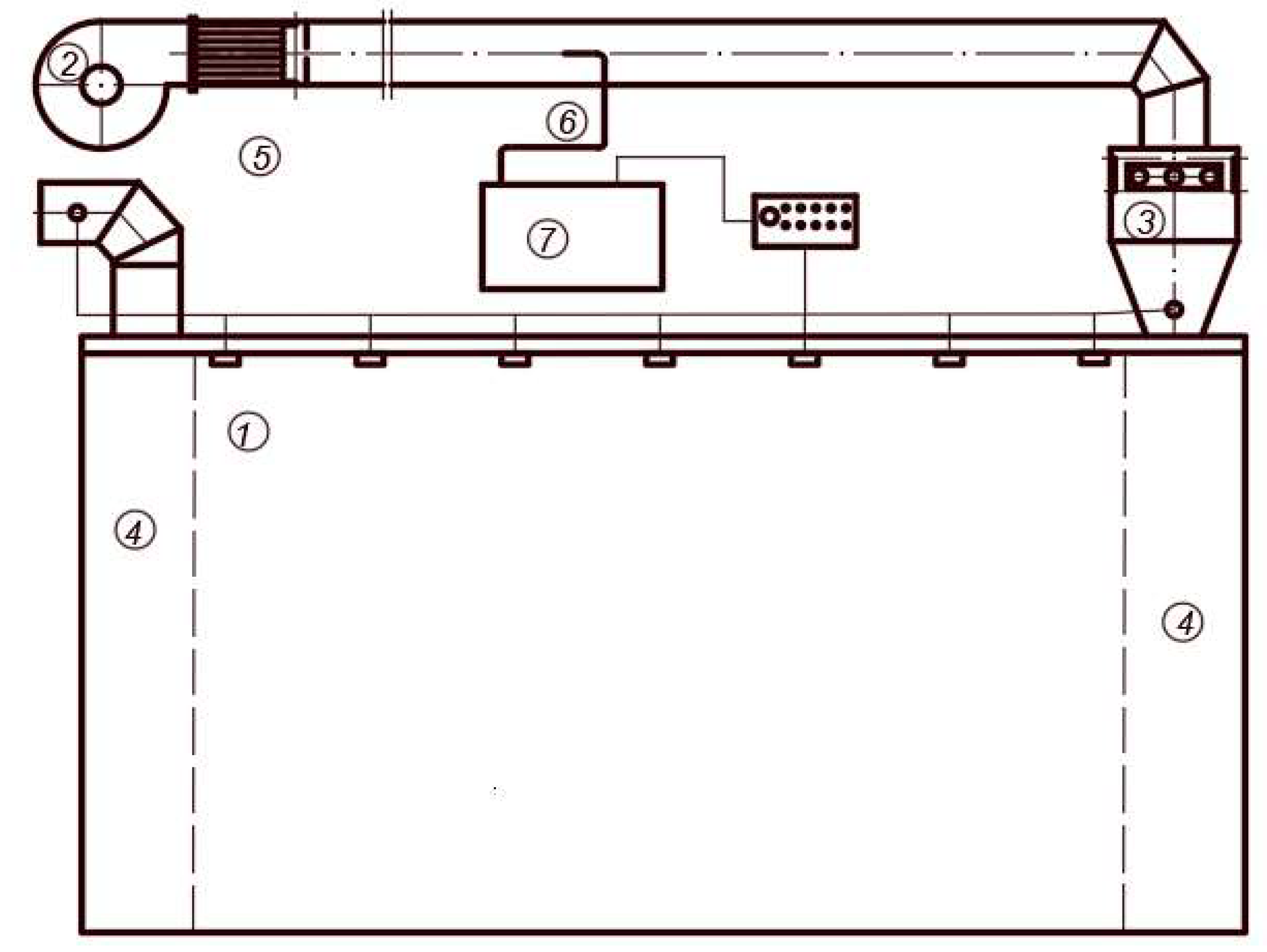
Figure 1. Test stand: 1—rock bed, 2—fan, 3—heater, 4—settling chambers, 5—elements stabilizing flow, 6—anemometer, 7—computer.
Applsci 11 10711 g001
Figure 2. Topology of the temperature measurement sensor layout.
Applsci 11 10711 g002
Figure 3. The structure of the model developed—MLP 4-7-1.
Applsci 11 10711 g003
Figure 4. The results of linear regression for the temperature values in deposit measured using Celsius scale and determined using the MLP 4-7-1 model in relation to the testing file (of data).
Applsci 11 10711 g004
Figure 5. The results of absolute error for the temperature values determined using the MLP 4-7-1 model in relation to the testing file.
Applsci 11 10711 g005
Figure 6. Temperature distribution in dimensionless function of deposit height and time for definite dimensionless value X = 0 and Y = 0 (according to Figure 2) obtained from the model MLP 4-7-1 network.
Applsci 11 10711 g006
Figure 7. Temperature distribution in dimensionless function of deposit height and time for definite dimensionless values X = 0 and Y = 0 (according to Figure 3) obtained from the model MLP 4-10-1 network.
Applsci 11 10711 g007
Table 1. Input and output variables.
NameDesignationUnit
Input signals (4 variables)
1x coordinates of the locationXNon dimensional
2y coordinates of the locationYNon dimensional
3z coordinates of the locationZNon dimensional
4Timet[h]
Output signal (1 variable)
5TemperatureT[°C]
Table 2. A fragment of the training file for the ANN simulator (T—output variable).
No.XYZt [h]T [°C]
3310.65110.50.57.13342.55
3320.65110.50.57.30042.53
3330.65110.50.57.46642.50
3340.65110.50.57.63342.48
3350.65110.50.57.80042.46
3360.65110.50.57.96642.46
3370.65110.50.58.15042.43
Table 3. Regressive statistics both for the selected model and the rejected models, for training set, validation set and testing set, respectively.
MLP 4-7-1
Regression StatisticsT for Training FileT for Validation FileT for Testing File
Data Mean37.857437.949937.4636
Data S.D.4.80595.05274.9947
Error Mean−0.0002−0.0120−0.0181
Error S.D.0.26050.27800.2806
Abs Mean0.19230.21070.2082
S.D. Ratio0.05420.05500.0562
Correlation0.99850.99850.9984
MLP 4-10-1.
Regression StatisticsT for Training FileT for Validation FileT for Testing File
Data Mean37.677638.024137.7491
Data S.D.5.03884.77794.8083
Error Mean00.0040−0.0058
Error S.D.0.14380.16270.1579
Abs Mean0.10460.10790.1073
S.D. Ratio0.02850.03410.0328
Correlation0.99960.99940.9995
MLP 4-5-1.
Regression StatisticsT for Training FileT For Validation FileT for Testing File
Data Mean37.932337.761537.5023
Data S.D.4.87524.69025.2108
Error Mean00.0980.0197
Error S.D.0.43260.44660.4554
Abs Mean0.34450.34540.3557
S.D. Ratio0.08870.09520.0874
Correlation0.99610.99550.9962
Publisher’s Note: MDPI stays neutral with regard to jurisdictional claims in published maps and institutional affiliations.