Review

Weed Detection in Rice Fields Using Remote Sensing Technique: A Review

1
Department of Agriculture Technology, Faculty of Agriculture, Universiti Putra Malaysia (UPM), Serdang 43400, Malaysia
2
Department of Civil Engineering, Faculty of Engineering, Universiti Putra Malaysia (UPM), Serdang 43400, Malaysia
3
Department of Electrical and Electronic Engineering, Faculty of Engineering, Universiti Putra Malaysia (UPM), Serdang 43400, Malaysia
4
Department of Biological and Agricultural Engineering, Faculty of Engineering, Universiti Putra Malaysia (UPM), Serdang 43400, Malaysia
5
Institute of Tropical Agriculture and Food Security (ITAFoS), Universiti Putra Malaysia (UPM), Serdang 43400, Malaysia
6
Department of Crop Science, Faculty of Agriculture, Universiti Putra Malaysia (UPM), Serdang 43400, Malaysia
*
Author to whom correspondence should be addressed.
Appl. Sci. 2021, 11(22), 10701; https://doi.org/10.3390/app112210701
Submission received: 10 September 2021 / Revised: 31 October 2021 / Accepted: 1 November 2021 / Published: 12 November 2021
(This article belongs to the Special Issue Sustainable Agriculture and Advances of Remote Sensing)

Abstract

:
This paper reviewed the weed problems in agriculture and how remote sensing techniques can detect weeds in rice fields. The comparison of weed detection between traditional practices and automated detection using remote sensing platforms is discussed. The ideal stage for controlling weeds in rice fields was highlighted, and the types of weeds usually found in paddy fields were listed. This paper will discuss weed detection using remote sensing techniques, and algorithms commonly used to differentiate them from crops are deliberated. However, weed detection in rice fields using remote sensing platforms is still in its early stages; weed detection in other crops is also discussed. Results show that machine learning (ML) and deep learning (DL) remote sensing techniques have successfully produced a high accuracy map for detecting weeds in crops using RS platforms. Therefore, this technology positively impacts weed management in many aspects, especially in terms of the economic perspective. The implementation of this technology into agricultural development could be extended further.

1. Introduction

It is undoubtful that weeds, also known as invasive plants, have their roles in the ecosystem. However, their presence in crops such as rice, oil palm, rubber, and other mass plantations influences productivity, causes significant economic consequences, decreases land prices, and reduces company profits [1]. Moreover, the current trend shows that farmers worldwide are strongly dependent on herbicides used to control weeds; other control measures include cultural, physical, biological, and mechanical methods [2].
A statistic released by the Food and Agriculture Organization of the United Nations (FAO) for the years 1990 to 2019 showed that the Asia continent had used approximately 805,412 tonnes of herbicides in controlling the presence of weeds in various types of crops, followed by the Americas (593,619 tonnes), Europe (179,799 tonnes), Oceania (29,309 tonnes), and Africa (21,117 tonnes) [3]. Thus, much money was spent on herbicides to control and manage the presence of weeds in crops. However, too much dependence on herbicides usage to control weeds to maximize yield production has caused herbicide resistance and reduced the choices of herbicides to use [4,5]. Figure 1 illustrates the herbicides usage in controlling weeds for each continent in percentage.
It is necessary to construct systematic and strategic planning to improve the precision agriculture (PA) sector, especially in weed management, to control and increase yield production, leading to a better economy for the country and farmers. Therefore, remote sensing-based techniques were used to construct and optimize weed management. Remote sensing is a comprehensive framework that monitors and captures earth surface images without direct contact with it. In PA sectors, the data gathered can be used in various applications, such as monitoring rice’s morphology [6], yield estimation [7], and mapping irrigated areas for food security and water resource management [8]. However, even though remote sensing has been widely used in weed management, it may not be a permanently adopted by developing countries anytime soon since local farmers still prefer the traditional practices.
Thus, this paper aims to review and discuss the techniques and algorithms used in remote sensing to construct systematic and strategic planning to improve precision agriculture in weed management. As a result, researchers can adapt the knowledge of controlling weed presence and increasing yield production, especially in developing countries. This study’s focus was limited to weed detection using a remote sensing platform in the paddy field. However, weed detection in other crops using remote sensing was also included.
This paper is organized into eight sections. Section 1 briefly explains this study’s goal in implementing remote sensing techniques into the precision agriculture (PA) sector. Section 2 explains the strategy used to search through the scientific database for relevant publications. Meanwhile, Section 3 discusses the importance of rice and what has been carried out to increase yield. Section 4 highlights the best stage to control weed in paddy, weed types, and traditional farming practices. Section 5 presents the literature covering various types of weed detection using remote sensing techniques. Section 6 reviews the impact of inadequate and good weed management on crops, yield, and economy. Section 7 deliberates the future direction of remote sensing techniques in weed detection. Lastly, in Section 8, the conclusions are presented.

2. Methodology

Articles were searched and identified from nine bibliographic databases: IEEE, Science Direct, MDPI, Web of Science, Scopus, Google Scholar, ProQuest, Springer, and Wiley Online Library. The primary keyword ‘remote sensing’ and its synonyms were paired with the secondary keyword ‘weed’ and the third keyword ‘detection’ and its synonyms, with Boolean operators. These keyword sets were used in each database search. In addition, a hand search was also run to ensure no related articles were missed. The search was conducted in the quarter of 2021.
All search results were filtered based on five criteria: (1) the study must use remote sensing imagery and platform as the primary data input with at least three spectral bands (red, green, and blue), (2) the study must discuss the application of remote sensing techniques in weed detection, (3) the document must have reported the research conducted, (4) the included documents have been published up to the quarter of 2021, and (5) the articles must be in English.
Next, the articles were screened by title and abstract to eliminate articles that did not meet the stated criteria. Finally, the full text of the remaining articles was carefully reviewed to decide whether they met the criteria or not. Lastly, details from selected articles were extracted and compiled into one giant spreadsheet. The details include citation information, study objective, remote sensing sensor, crop and weed types, approaches and technique used, accuracy assessment, study’s implications, year of publication, and reference data.

3. The Importance of Rice Productivity

Rice is consumed by around 3.5 billion people worldwide. However, the estimated demand by 2025 is mind-boggling, as rice consumption would grow higher than the population growth in major Asian countries [9]. In general, paddy production had increased globally up to 12% from 1975 to 2008, and nearly 166 million ha of paddy have been harvested in the world [10]. However, in 2020, it was reported that China was the leading country in the world producing paddy (30.5%), followed by India (224.14%), Bangladesh (7.36%), Indonesia (7.14%), Vietnam (5.53%), and Thailand (4.17%) [11].
Numerous research have been conducted to increase the yield of rice production to fulfil consumer demand. Masum et al. [12] had found that the Boterswar variety could help improve the weed-suppressing capacity of rice. The study used five Bangladesh rice varieties named Boterswar, Goria, Biron, Kartiksail, Hashikolmi, and Holoi, and these varieties were planted via a non-weed control method. By using Simpson’s diversity ndex (SDI) to measure the infestation rate of weed species, the relative neighbour effect (RNE), and relative competitive intensity (RCI), results showed that Boterswar facilitated the crop–weed interaction compared to the other varieties. This finding will significantly influence methods to control the presence of weeds in paddy fields.
Meanwhile, Yamori et al. [13] found that, to increase plant productivity among various crop species, they must improve the photosynthesis rate at the single-leaf level. To achieve this, they used transgenic rice plants that consist of various amounts of the Rieske FeS protein in the cytochrome (cyt) b6/f complex at between 10 and 100% of wild-type levels. As a result, they decreased the electron transport rates through photosystem II, leading to an increased uptake of carbon dioxide (CO2) and a successfully increased production yield, up to 40% [14].
Besides improving the photosynthetic activities, improving the irrigation system in paddy is the best practice to increase yield. In Thailand, they practiced an alternate wetting and drying (AWD) method [15]. By setting the threshold at 15 cm of water level below the soil surface for irrigation, this method increased the grain yield by 15% in the wet season and 7% in the dry season, meanwhile improving water usage by 46% and 77% in the wet and dry season, respectively, compared to continuously flooding water into the paddy field. Therefore, the AWD method is a good practice that helps sustain rice production through water-saving. Lahue et al. [16] also obtained the same result, and in addition, their study successfully reduced the total arsenic concentration released by rice grain up to 65%. Meanwhile, Liang et al. [17] managed to reduce the methane emissions into the atmosphere by up to 77.1%.
Climate conditions played a significant role. The potential rice yield will be affected by severe climate conditions due to increased sterility caused by heat and shortening of the growing season [18]. Van Oort [19] implemented a geographical information system (GIS) by producing a map of abiotic stresses in Africa using drought, cold, iron toxicity, and salinity or sodicity information as the input. From the analysis, drought was found as the most critical variable that contributes to stress, where 33% of rice area was potentially affected, followed by iron toxicity (12%), and then cold (7%) and salinity/sodicity (2%). Dossou-Yovo et al. [20] used socio-economic, biophysical, farmer population surveys, and secondary remote sensing data on soil characteristics and demand for water to determine drought input parameters in rice-based inland valley production systems. Their study shows that the average annual standardized precipitation evapotranspiration index and groundwater availability duration were the most critical input to determine drought occurrence in their study area.
It is crucial to find solutions to improve and increase rice yield. However, to achieve rice production sustainably and meet demands, productivity and quality must significantly improve. Therefore, through participatory approaches, it is critical to foster joint working between research, extension, local governments, non-governmental organizations (NGO), and private industry to identify the relevant constraints to high yield, adopt new solutions and technologies, and make systematic decisions to close rice yield gaps.

4. Controlling Weed in Paddy Fields at Different Growth of Stages

In general, rice growth periods can be identified in three stages. They are the vegetative stage, reproductive stage, and maturative or ripening stage [21]. Depending on agricultural and environmental conditions, the whole cycle takes about 120 to 125 days. The International Rice Research Institute (IRRI) splits the growth cycle into five stages [22]. A general idea of the growth cycle is presented in Figure 2, with morphology examples.
Rice is generally a weak competitor with weeds. Therefore, the vegetative stage is critical in the paddy growth cycle. Successfully controlling weeds at this stage can deliver a 95% weed-free yield [23]. This is agreed with by Kamath et al. [24] because the effect of weeds in this stage will be at maximum. However, if we fail to prevent weeds from spreading in the vegetative stage, they will dominate the area, leading to a lack of sufficient space, light, and nutrients to grow and develop [25]. As a result, crops will experience uneven flowering and will not mature uniformly for the scheduled harvest [26,27].
Once the tillering reaches its maximum number, the reproductive stage will occur, followed by the maturative or ripening stage. Excess water in the fields is drained, resulting in a drop in the overall biomass due to lower moisture content. The grain is maturing and becoming heavier. At this stage, the presence of weeds will not affect the development of the crop. Nevertheless, we cannot save the yield losses because weeds dominated the paddy plot and the number of paddy crops that survive the competition is nominal. In general, weed in paddy can be classified into three types. They are grasses, sedges and broad leaved weeds [28], and Table 1 shows a compilation of the primary weeds usually found in paddy fields.
The environmental relationship between weed and rice is very complicated and complex [29]. The weed management system needs improvement to control the spreading of weeds. The traditional practices that include burning, hand sowing, manual spot spraying, herbicide pre-emergence or post-emergence application, and repetitive blade hoeing are not practical anymore. These practices impacted the non-target species and the ecosystem rather than benefiting production [30].
The traditional weed sampling for practice-oriented management is too costly, and this is not a recent concern. Since 2005, Brown and Noble [31] have developed automated methods for evaluating infestation. Automatic weed sampling provides a way to increase the amount of data obtained in the field (smaller sampling intervals) at lower overall costs of 7–13 USD/ha, and sensor technology is used exclusively for the application of herbicides, resulting in a reduction of herbicide usage of 30–70% [32].
Advanced weed management methods are required to manage weeds effectively. The process may include targeted and site-specific weed control, selection of weed seeds, different herbicide application (depending on weed distribution, spatial arrangement and soil properties), destruction of weed seeds over predation and microbial loss, nano herbicides, and optical spraying techniques. Advanced vision-guided robotics that can be adopted for site-specific weed management (SSWM) are transgenic herbicide-resistant crops, weed control and spraying robots, decision support systems, and pattern recognition modelling [33]. Implementing these technologies will help prevent unwanted species and improve existing weed management systems [34].

5. Weed Detection Using Remote Sensing Technique

Remote sensing technology aims to monitor and capture the earth’s information without making direct contact and destroying it. The utilization of the electromagnetic spectrum, ranging from visible to microwave for measuring the earth’s properties, is the main idea behind remote sensing technology. Since the target’s reactions to various wavelength regions differ, we can exploit them to identify vegetation, water, soil, and other features [35]. Combining the target’s reaction with the shape, texture, and pattern information of weeds and crops, we can discriminate them and improve SSWM using remote sensing algorithms.
The image processing workflow to detect weed in paddies can generally be divided into five stages: image data collection, pre-processing, feature extraction and selection, training, image classification and validation [36].

5.1. Image Data Collection

There are multiple platforms available for data gathering for weed detection in crops, such as digital cameras [37], hand-held spectroradiometers [38], polarization spectroscopy [39], and satellites [40]. However, unmanned aerial vehicles (UAV) are the most popular platforms researchers use to identify weeds in crops, due to their availability, high-quality data delivery, and ease of handling [41]. Nevertheless, the data collection differs in the types of sensors attached to UAVs: RGB, multispectral, or hyperspectral.

5.1.1. RGB Sensor

The RGB sensor is the most widely used and widely available commercial camera. Because of their promise in delivering high-quality images and low-cost operational needs, their possible applications have been the focus of most research for many years [42,43]. These sensors are increasingly employed in machine learning algorithms for object recognition, diseases, phenology, and other applications.
These are typical steps to acquire RGB images captured by UAV remote sensing: (1) pre-flight planning, (2) flight and image acquisition and (3) post-processing and indices or dataset extrapolation [44]. However, when preparing the images for machine learning algorithms, the processing steps are different depending on the research’s objective [45,46,47]. The advantage of using this sensor is that radiometric and atmospheric calibration are not required, unlike multispectral and hyperspectral images [41]. Therefore, noises from electromagnetic radiation (EMR) can be ignored.

5.1.2. Multispectral Sensor

The use of the multispectral sensors has become a trend nowadays because it has more than three (RGB) bands installed. Compared to RGB sensors, several vegetation indices that can be investigated are significantly expended. Nevertheless, to obtain accurate indices, radiometric and atmospheric calibration are compulsory. Moreover, unlike RGB sensors, the multispectral sensor is unable to deliver a high-quality spectral resolution image. This drawback can be overcome by using a lower flying height and acceptable percentage of horizontal and vertical image overlap [48].
In general, the typical steps involved in preparing multispectral images captured by UAV remote sensing are: (1) radiometric and atmospheric calibration, (2) locating and avoiding input and output (I/O) errors, missing data, and mission failure, and (3) image rectification, georeferencing, and stacking [41]. In addition, these sensors are increasingly being employed in machine learning algorithms for site-specific weed management (SSWM) [40,49,50].

5.1.3. Hyperspectral Sensor

The hyperspectral sensor analyzes a broad spectrum of light, instead of assigning primary colors (red, green, and blue). These sensors can record hundreds of narrow radiometric spectral bands from visible to infrared, sometimes up to microwave ranges. Its ability in providing narrow radiometric spectral bands can detect specific field concerns. Thus, users can compute narrowband indices, such as the chlorophyll absorption ratio index (CARI), transformed chlorophyll absorption ratio index (TCARI), triangular vegetation index (TVI), and photochemical reflectance index (PRI) [51].
Preparing hyperspectral data is more complicated than RGB and multispectral sensors because its radiometric and atmospheric calibration workflows are more complex. Sensor calibration approaches are generated from the UAV’s hyperspectral platforms, which use simulated targets to check data quality, correct radiance, and provide high-quality reflectance information [52]. Therefore, typical steps in acquiring and preparing hyperspectral data captured by UAV remote sensing are: (1) setting up a flight plan, (2) image size and data storage, and (3) quality assessment [41]. Table 2 summarizes the characteristics of each sensor alongside its advantages and disadvantages.

5.2. Image Mosaicking and Calibration

Images acquired from UAVs can be mosaicked using a Pix4D mapper (Pix4D, Prilly, Switzerland), Agisoft Photoscan Pro (Agisoft LLC, 52 St. Petersburg, Russia), and any available commercial software to generate qualitative, high-resolution orthomosaic images. After mosaicking, the process will continue with radiometric calibration and rescale the intensity of the electromagnetic radiation or digital number (DN) into the percentage of reflectance values [53]. Researchers have implemented numerous methods, such as the traditional empirical line correction approach and modern automatic radiometric calibration using available commercial software.
The empirical line correction approach is an atmospheric correction technique that provides a straightforward surface reflectance calibration method, if a set of invariants in the time calibration target measurement is provided. Kelcey and Lucieer [54] implemented this approach to improve six multispectral UAV data quality bands for quantitative data analysis. Similarly, Mafanya et al. [55] applied the same method and obtained a reflectance value of r = 0.997 (p ≤ 0.01) with an overall root mean square of 0.63. Nevertheless, when dealing with high-quality data, the performance and accuracy must be re-evaluated [56].
In order to improve radiometric calibration accuracy, Xu et al. [57] introduced a spectral angle correction approach, where their method uses all information in each spectral band. Compared to the empirical line correction approach, they successfully improved the mean relative percent error (MRPE) range up to 3% in the visible band and 1% in the near-infrared (NIR) band. This finding will highly benefit the agriculture remote sensing field.
However, the user can also run the radiometric calibration automatically using available commercial software such as Agisoft Photoscan Pro (Agisoft LLC, 52 St. Petersburg, Russia) and Pix4D mapper (Pix4D, Lausanne, Switzerland). The ‘reflectance map’ tool in Pix4D mapper software is similar to calibrate ‘calibrate reflectance’ in Agisoft Photoscan Pro that employs multiple image attributes to determine surface reflectance [58]. In addition, these software packages provide ‘color correction/balancing’ functions to develop the image information based on a radiometric block correction algorithm. However, the algorithms used in these packages only calculate the neighbouring image’s histogram homogeneity, not the bidirectional reflectance distribution function (BRDF) effect in a single image [59].

5.3. Feature Extraction and Selection

Following the spectral calibration, feature extraction can be extracted or computed for different image processing purposes using various approaches (Table 3). This process will be helpful for the classification and identification of weeds in paddy fields. Feature extraction techniques are beneficial, especially in shape and pattern recognition. As features define the behavior of an image, they show its place in terms of storage taken, classification efficiency, and, obviously, in time consumption [60]. Therefore, optimizing the feature subset is required before feeding it into the machine learning (ML) and deep learning (DL) algorithms for improving the classification process and making it cost and time-efficient [61].

5.4. Image Classification and Validation

Many machine learning (ML) and deep learning (ML) algorithms are available for image classification. However, choosing the best one that fits the research’s objective is crucial, because different algorithms have different difficulty levels. Therefore, Section 5.6 will further discuss the application of remote sensing algorithms in detecting weeds in crops.
Accuracy assessment is crucial to validate the quality of the classification output that best represents the study area. Overall, the assessment can be carried out by comparing the classified pixels with ground truth pixels using a confusion matrix [67]. The result for weed classification is presented in terms of producer accuracy and overall accuracy. Producer accuracy (Equation (1)) is the probability that a pixel in the classification correctly shows class X. Given the ground truth class is X, producer accuracy can be calculated using
P r o d u c e r   a c c u r a c y = c a a c . a   ×   100 %
where:
-
caa = element at a position ath row and ath column.
-
c.a = column sums.
Overall accuracy (Equation (2)) is the total percentage of pixels correctly classified, and it can be calculated by using
O v e r a l l   a c c u r a c y = a = 1 U c a a Q   ×   100 %
where:
-
Q = total number of pixels.
-
U = total number of classes.
The agreement between variables with ground truth data can be represented by using the kappa coefficient (Equation (3)), and its value can be calculated by using
K a p p a   c o e f f i c i e n t ,   K = a = 1 U c a a Q a = 1 U c a . c a Q 2 1 a = 1 U c a . c a Q 2   ×   100 %
where:
-
ca = row sums.
However, some limitations occur when dealing with object-based classification, primarily related to the real-world object recognition’s thematic and geometrical accuracy [68]. Therefore, to address this concern, De Castro et al. [46] designed Weed detection Accuracy (WdA), Equation (4). This index analyzes the spatial placement of classified weeds by using the intersection of shapefiles as a spatial relationship rather than the overall overlap.
W d A   % = A r e a   o f   O b s e r v e d   W e e d   o b j e c t s   i n t e r s e c t i n g   D e t e c t e d   W e e d   O b j e c t s A r e a   o f   O b s e r v e d   W e e d   ×   100
The detection of weeds is crucial for successful site-specific weed management (SSWM). However, weed detection is still challenging for automatic weed removal [37]. In addition, low tolerance between the cutting point and the crop location requires an accurate weed classification against the main crop. Therefore, several works have been conducted in the context of remote sensing image processing to detect and improve site-specific management [69,70,71].

5.5. An Overview of Machine Learning in Agriculture

In recent years, machine learning (ML) has provided a new criterion for agriculture with big data technology and high-performance computing. The development of ML has created new opportunities in agriculture operational management to unravel, measure, and analyze complex data [72]. Generally, the ML framework involves learning from ‘experience’, known as training data, to execute the classification, regression, or clustering tasks. These training data are usually regarded as a feature described by a set of attributes or variables. The machine learning model works by predicting the pattern and trend of future events in crop monitoring and assessment [73]. The ML model’s performance in a particular task is evaluated by performance metrics improved by experience over time. As a result, classification techniques have been a prominent research trend in machine learning for many years, informing various studies. This method seeks to create features from the input data. Furthermore, it is highly field-specific and requires significant human effort, leading to deep learning techniques [36]. Figure 3 shows how machine learning and deep learning techniques work.
Deep learning is a subset of machine learning, but with more complicated image analysis [36], commonly used in agricultural crop monitoring and management. In terms of functionality, machine learning and deep learning share the same purpose: to make intuitive and intelligent decisions using artificial neural networks stacked layer-wise based on what it has learned while being trained [74]. However, in terms of developing an accurate model, machine learning requires a pre-processing stage before the model is developed, trained, and validated. In contrast, deep learning has a ‘build in’ feature extractor to extract meaningful features from the raw data. It learns features layer by layer, which means that it learns low-level features in the first levels and then progresses up the hierarchy to learn a more abstract representation of the input. [75]. Regardless of which agricultural domain and purpose, it has taken a directive in various crop monitoring purposes such as nutrient disorder, weed detection, plant insects, and disease detection. Many studies on weed detection have utilized deep learning with other remote sensing methods concerning classification or regression performance differences. The outcome has marked high accuracy, outperforming other commonly used image processing techniques [76].
In deep learning (DL), CNN is the most well-known and widely used algorithm [69,70,77]. The fundamental advantage of CNN over the other DL algorithms is that it automatically detects significant elements without the need for human assistance (36). Comparable to the multi-layer perceptron (MLP), where it consists of three layers known as the input, output, and hidden layer [78], CNN has many convolution layers before sub-sampling (pooling) layers, with fully connected (FC) layers as the last layers. An illustration of the CNN framework for image classification is shown in Figure 4.
A CNN model’s input image is structured in three dimensions: height (m), width (m), and depth (r), where height (m) equals the width (m), and the depth (r) is referred to as channel number. For example, the depth (r) of the RGB image in Figure 4 equals three (three bands). The available kernel filters for the convolution layer will be designated by the letter k (n × n × q). However, n must be less than m, and q must be equal to or less than r. The dot product between the input and the weights is calculated by the convolution layer using Equation (5)
h k = f W k * x + b k
where:
-
h k = feature maps in size (m – n – 1).
-
W k = weightage.
-
b k = bias.
These groundbreaking CNNs were able to achieve such incredible accuracy, partly because of their non-linearity. The rectified linear activation function (ReLU) applies the much-needed nonlinearity to the model. Non-linearity is necessary to produce a non-linear decision boundary, so the output cannot be written as a linear combination of the inputs. If there is no non-linear activation function, the deep CNN architecture will evolve into a single equivalent convolutional layer, and its performance will hardly be so. The ReLU activation function is used explicitly as a non-linear activation function, in contrast to other non-linear functions such as Sigmoid, because it has been observed from experience that the CNN using ReLU trains faster than the corresponding CNN [79]. Furthermore, the ReLU activation function is a one-to-one mathematical operation, as shown in Equation (6).
R e L U x   = m a x 0 , x
It converts the whole values of the input to positive numbers. Thus, lower computational load is the main benefit of ReLU over the others. Subsequently, each feature map in the sub-sampling layers is down-sampled, decreasing network parameters, speeding up the learning process, and overcoming the problem related to the overfitting issue. This can be carried out in the pooling layers. The pooling operation (maximum or average) requires selecting a kernel size p × p (p = kernel size) and another two hyperparameters, padding and striding, during architecture design. For example, if max-pooling is used, the operation slides the kernel with the specified stride over the input, while only selecting the most significant value at each kernel slice from the input to yield a value for the output [80].
Padding is an important parameter when the kernel extends beyond the activation map. Padding can save data at the boundary of the activation maps, thereby improving performance, and it can help preserve the size of the input space, allowing architects to build simpler higher-performance networks, while stride indicates how many pixels the kernel should be shifted over at a time. The impact that stride has on a CNN is similar to kernel size. As stride is decreased, more features are learned because more data are extracted [36]. Finally, the fully connected (FC) layers receive the medium and low-level features and generate the high-level generalization, representing the last-stage layers similar to the typical neural network’s technique. In other words, it converts a three-dimensional layer into a one-dimensional vector to fit the input of a fully connected layer for classification. Usually, this layer is fitted with a differentiable score function, such as softmax, to provide classification scores. The fundamental purpose of this function is to make sure the CNN outputs the sum to one. Thus, softmax operations are helpful to scale the model output into probabilities [80].
The key benefit of the DL technique is the ability to collect data or generate a data output using prior information. However, the downside of this strategy is that, when the training set lacks samples in a class, the decision boundary may be overstrained. Furthermore, given that it also involves a learning algorithm, DL consumes many data. Nevertheless, DL requires enormous data to build a well-behaved performance model, and as the data grow, the well-behaved performance model can be achieved [36].

5.6. The Application of Remote Sensing and Machine Learning Technique into Weed Detection

Choosing remote sensing (RS) and machine learning algorithms for SSWM can improve precision agriculture (PA). This situation has resulted in integrating remote sensing and machine learning becoming critical, as the need for RGB, multispectral, and hyperspectral processing systems has developed. Numerous researchers who tested the RS technique successfully produced an accurate weed map with promising implications for weed detection and management. Since the weed management using RS technique application in paddy is still in its early stage, Table 4 lists more studies on weed detection and mapping in various crops that apply remote sensing techniques with acceptable accuracy, for further reviews.
Even though numerous platforms for data collection are accessible, a UAV is the best for identifying weeds in paddy because of its availability, high-quality data delivery, and convenience. On the other hand, the review discovered that deep learning (DL) is suitable for classifying grass weeds in paddy and producing high accuracy weed maps. However, when referring to other crops, it might differ for sedge and broad-leaved weeds. Nevertheless, this method necessitates a large amount of training data, resulting in vast agricultural datasets. In the future, to optimize the use of the RS technique, we must know what types of weeds we are dealing with in the paddy fields to choose the best technique for our research. Therefore, to classify weeds, a sophisticated method might not be necessary.

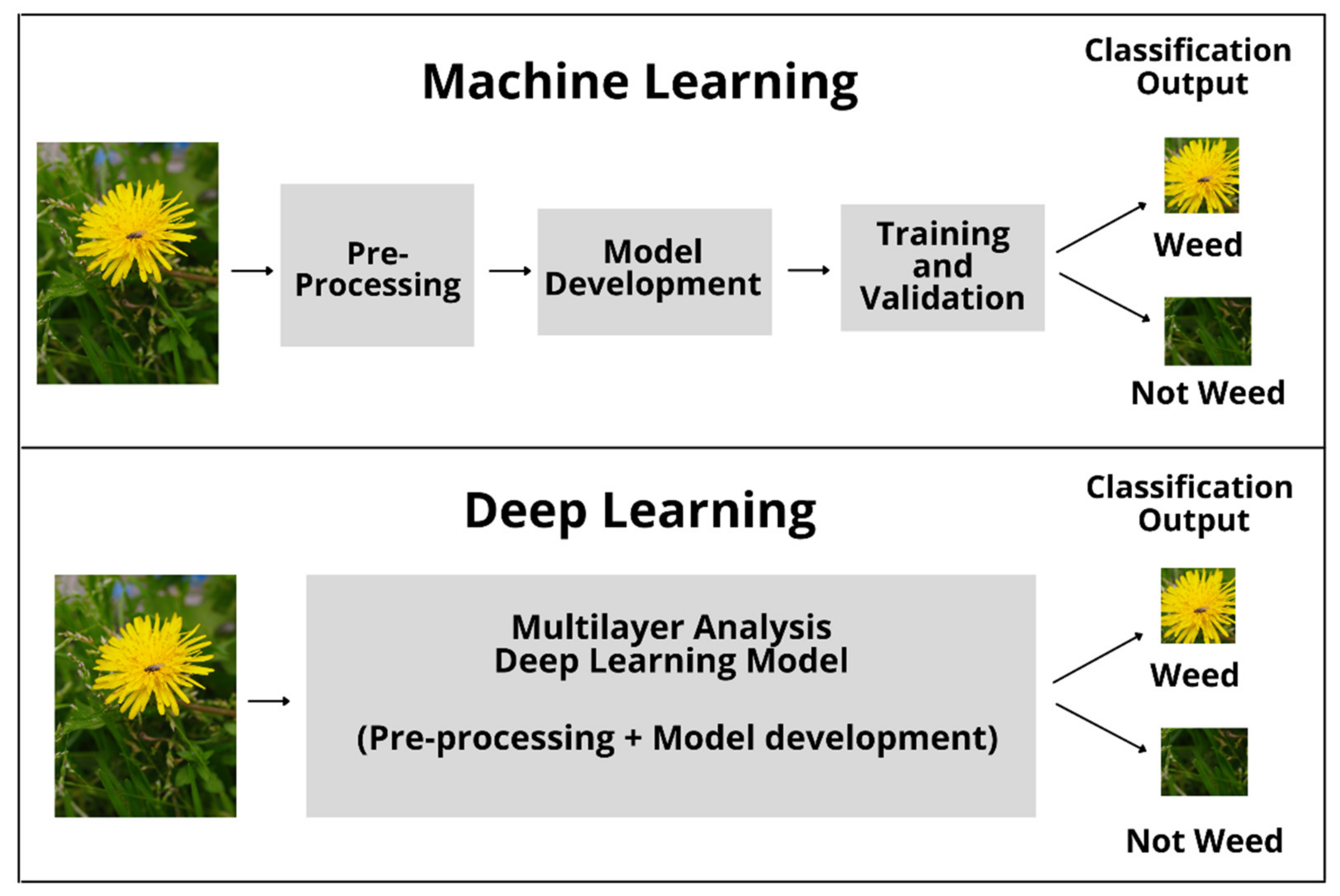
5.6.1. Machine Learning (ML)

Machine learning is a part of artificial intelligence that enables machines to recognize patterns and judge with little or no human input. Back during the early introduction to machine learning, Aitkenhead et al. [81] proposed a simple morphological characteristic measurement of a leaf shape (perimeter2/area) and a self-organizing neural network to discriminate weeds from carrots using a Nikon Digital Camera E900S. Their proposed method enables the system to learn and differentiate between species with more than 75% accuracy without predefined plant descriptions. Eddy et al. [86] tested an artificial neural network (ANN) to classify weeds (wild oats, redroot pigweed) from crops (field pea, spring wheat, canola) using hyperspectral images. The original data were 61 bands that were reduced to seven bands using principal component analysis (PCA) and stepwise discriminant analysis. A total of 94% overall accuracy was obtained from the ANN classification. Yano et al. [90] also successfully classified weeds from sugarcane using ANN with an overall accuracy of 91.67% with a kappa coefficient of 0.8958.
Barrero et al. [45] investigated the use of artificial neural networks (ANN) to detect weed plants in rice fields using aerial images. To train the algorithm with a flying height of 50 m, they used a gray-level co-occurrence matrix (GCLM) with Haralicks descriptor for texture classification and a normalized difference index (NDI) for color. As a result, they successfully obtained 99% precision for detecting weed on the test data. However, the detection level was low for weeds similar to rice crops, because the image resolution was 50 m above the ground. Later, to evaluate the ANN’s performance, Bakhshipour and Jafari [37] used a digital camera to detect weeds using shape features with an improved machine learning algorithm, support vector machine (SVM). Results showed that SVM outperformed the AAN with an overall accuracy of 95.00%, while 93.33% of weeds were correctly classified. Meanwhile, for ANN, its overall accuracy was 92.92%, where 92.50% of weeds were correctly classified.
Doi [84] used ML knowledge to discriminate rice from weeds from paddy fields by overlapping and merging 13 layers of binary images of red-green-blue and other color components (cyan, magenta, yellow, black, and white). These color components were captured using a digital camera (Cyber-shot DSC T-700, Sony) and used as input to specify the pixels with target intensity values based on mean ranges with ±3× standard deviation. The result shows that yellow with 1x standard deviation has the best target intensity values in discriminating paddy from weeds, with improved ratio values from 0.027 to 0.0015.
Shapira et al. [85] used general discriminant analysis (GDA) to detect grasses and broad-leaved weeds among cereal and broad-leaved crops. Using spectral relative reflectnce values obtained by field spectroscopy as references, total canopy spectral classification by GDA for specific narrow bands was 95 ± 4.19% for wheat and 94 ± 5.13% for chickpea. Meanwhile, for vegetation and environmental monitoring on a new micro-satellite (VENμS), total canopy spectral classification was 77 ± 8.09% for wheat and 88 ± 6.94% for chickpea, and for the operative satellite advanced land imager (ALI) it was 78 ± 7.97% for wheat and 82 ± 8.22% for chickpea. Thus, an overall classification accuracy of 87 ± 5.57% for >5% vegetation coverage in a wheat field was achieved within the critical timeframe for weed control, thus providing opportunities for herbicide applications to be implemented.
Meanwhile, Rasmussen and Nielsen [95] developed a yield loss due to weed infestation model by combined manual image analysis, automated image analysis, image scoring, field scoring, and weed density data to estimate yield loss by weeds (Cirsium arvense) in a barley field on UAV images. With a flying height of 25 m above the ground, they successfully computed the model (Equation (7)) and found that grain moisture increased directly proportional to weed coverage (Equation (8))
Y = 100 · 1 exp   ( 0.0017 · X
where:
  • Y = Percentage of crop yield loss.
  • X = Percentage of weed coverage.
M = 0.0310 · X
where:
  • M = Proportional percentage increase in grain moisture.
  • X = Proportional percentage of weed coverage.
Other than artificial neural networks (ANN), support vector machine (SVM), and simple ML algorithms, other algorithms have been tested to detect and classify weeds from crops. They are maximum likelihood (ML), random forest (RF), vegetation indices (VIs), and discriminant analysis (DA) algorithms. De Castro, López-Granado, and Jurado-Expósito [83] used ML and VIs to classify cruciferous weed patches on a field-scale and broad-scale. Cruciferous weed patches were accurately discriminated against in both scales. However, the ML algorithm has a higher accuracy than VIs, 91.3 % and 89.45%. The same outcome was archived by Tamouridou et al. [89] when they classified Silybum marianum (L.) in cereal crops.
Fletcher and Reddy [38] explored the potential of a random forest algorithm in classifying pigweeds in soybean crops using a spectroradiometer (FieldSpec 3, PANalytical Boulder, Boulder, CO, USA) and WorldView-3 satellite data. One nanometer spectral data were grouped into sixteen multispectral bands to match them with the WorldView-3 satellite sensor. The accuracy of weed classifications ranged from 93.8% to 100%, with kappa values ranging from 0.93 to 0.97. The result shows an excellent agreement between the classes predicted by the models and the ground reference data. They also found that the most significant variable in separating pigweeds from soybean is the shortwave infrared (SWIR) band.
Similar to Baron, Hill, and Elmiligi [91] and Gao et al. [92], they used feature selection to train the random forest (RF) algorithm to classify weeds on different platforms: UAV RGB and hyperspectral camera, respectively. Their studies showed that the integration of feature selection with the RF algorithm produced an accurate map. As for Gao et al. [92], their output showed that for Zea mays, Convolvulus arvensis, Rumex, and Cirsium arvense weeds, the optimal random forest model with 30 significant spectral features would achieve a mean correct classification rate of 1.0, 0.789, 0.691, and 0.752, respectively. Meanwhile, Matongera et al. [40] tested discriminant analysis (DA) to classify and map invasive plant bracken fern distribution using Landsat 8 OLI. The performance of the classification output was compared with high spatial resolution data, WorldView-2 imagery. Worldview-2 classification outperformed Landsat 8 OLI with overall accuracies of 87.80% and 80.08%, respectively. However, for long term continuous monitoring, Landsat 8 OLI provides valuable information compared to the WorldView-2 commercial sensor.
A few researchers chose object-based image analysis (OBIA) to classify weeds from crops. OBIA is an automatic hierarchal image classification algorithm. It allows numerous image objects to be created and further categorized into user-defined classes [98]. For example, López-Granados et al. [87] used an RGB (red, green, blue) UAV to monitor early-season weeds in a sunflower field using object-based image analysis (OBIA). Their experiment was tested at two different flying heights, 30 m and 60 m, above the surface. They found that both flying heights give satisfactory outputs, with 2.5% to 5% thresholds and an accuracy higher than 85%. The same result was archived by López-Granados et al. [88], Mateen and Zhu [93], and Sapkota et al. [97] when they classified weeds from maize, wheat, and cotton, respectively. Their research helped farmers with rationalization of the herbicide application.
Some of the researchers integrated object-based image analysis (OBIA) with other machine learning algorithms. OBIA’s final output can be converted into another GIS format [99], making it flexible to integrate with other algorithms. For example, De Castro et al. [96] successfully classified Cynodon dactylon (bermudagrass) in a vineyard by combining OBIA with the decision tree (DT) algorithm. De Castro et al. [46] also managed to produce a weed map of Convolvulus arvensis L. (bindweed) in a soybean field by combining OBIA with the RF algorithm. Meanwhile, Che’Ya, Dunwoody, and Gupta [62] successfully generated various types of weed maps in the sorghum’s field by integrating OBIA with the artificial nearest neighbor (ANN) algorithm.
Kawamura et al. [47] experimented with the OBIA classification method using the simple linear iterative clustering algorithm–random forest (SLIC–RF). SLIC is a superpixel method for extracting input feature details for each subject. They used three-color spaces (RGB, hue-saturation-brightness (HSV) and transformation function of RGB images (CIE-L*a*b*)) as the primary input feature and a spatial texture, four VIs (excess green (ExG), excess red (ExR), green–red vegetation index (GRVI), and color index of vegetation extraction (CIVE)), and DSM as the secondary data. The HSV-based SLIC–RF outperformed the other color spaces tested, with an accuracy of 90.4%.
Instead of using an RGB UAV, Stroppiana et al. [50] used UAV multispectral images for early season weed mapping in rice using ISODATA classification. Their input data are spectral indices (normalized different vegetation index (NDVI), soil adjusted vegetation index (SAVI), GSAVI, a simple ratio index related to leaf pigments content and greenness (RGRI), normalized difference red edge (NDRE), and chlorophyll vegetation index (CVI)) and textural metrics. Weed mapping performance was validated by measuring overall accuracy (OA), while for weed class, omission errors (OE) and commission errors (CE) were calculated. The result shows that SAVI and GSAVI gave the best output compared to other indices, with 96.5% and 94.5% overall accuracy. The final production, classification map, weed proportion in the percentage map, weed canopy height measured in meters (m) map, and rice fraction cover map, were successfully produced from SAVI and GSAVI. Pantazi et al. [49] also chose multispectral UAVs to map weeds in cereals.

5.6.2. Deep Learning (DL)

Deep learning has recently become a machine learning component widely utilized in agricultural crop monitoring and management. It has taken a directive in many crop monitoring objectives such as weed detection, nutrient disorder, and disease detection. Huang et al. [43] utilized the fully convolutional network (FCN) method to map weeds in rice using unmanned aerial vehicle red-green-blue (UAV-RGB) imagery. Transfer learning was used to optimize the generalization capacity, and skip architecture was chosen to boost prediction accuracy. The result was then compared with the patch-based convolutional neural networks (CNN) algorithm and the pixel-based CNN method. The findings showed a proposed FCN method that outperformed others, both in efficiency and efficacy in terms of accuracy. The overall accuracy of the FCN method was up to 93.5%, and the accuracy for weed recognition was 88.3%.
Meanwhile, Huang et al. [94] also tested the same algorithm to delineate weeds from rice in multi-rotor UAV images. Using an RGB-UAV with a flying height of 10 m above the surface, they compared the object-based image analysis with the fully convolutional network (FCN). As expected, their finding shows that FCN performs better than OBIA, with an overall accuracy of 80.2% and 66.6%, respectively, which means that this algorithm can produce precise weed cover maps for the evaluated UAV-based RGB imagery.
Bah et al. [69] also tested other deep learning algorithms: convolutional neural networks (CNNs) on other crops, spinach, beet, and bean using UAV images to classify weeds in the crops from a 20 m flying height. The method effectively differentiates weeds from crops with an overall accuracy for beet of 93%, spinach of 81%, and bean of 69%. However, deep learning alone requires a great deal of training data. It is too time-consuming of a process to construct large agricultural datasets with pixel-level identifications by an expert. Therefore, Bah et al. [70] proposed a fully automatic learning method using CNNs with an unsupervised training dataset collection for weed detection from UAV images. The classification started with the identification of inter-row weeds from the automatic detection of crop rows. Then, training datasets from inter-row weeds were made before performing the CNNs to detect crop and weed images. Results obtained were compared with supervised training data, and the difference in accuracy for spinach is 1.5%, and for bean is 6%. The differences between supervised and unsupervised are narrow. This proposed method can be the best option, since supervised labelling is expensive and challenging and requires human expertise.
Dos Santos Ferreira et al. [71] evaluated the unsupervised deep learning performance to discriminate weeds from soybean in UAV images. They tested two unsupervised deep clustering algorithms, joint unsupervised learning of deep representations and image clusters (JULE) and deep clustering for unsupervised learning of visual features (DeepCluster), using two public weed datasets. The first datasets were captured in a soybean plantation in Brazil, and weeds were distinguished between the grass and broad leaf weed. Meanwhile, the second dataset consists of 17,509 labelled images of eight common species originating from Australia. Semi-automatic data labelling in agriculture was used to evaluate the outputs, and the result showed that this method achieved up to 97% accuracy, reduced 100 times in manual annotations.
This study has used the shape, texture, and pattern of weeds and crops trained and classified by remote sensing algorithms. However, more research needs to be carried out to detect and produce an accurate weed coverage map that recognizes weed types: grass, sedge and broad-leaved in the paddy field. This is because different weeds have different characteristics that require other variables to identify them. Nevertheless, based on the previous study, it is not impossible to produce an accurate map that will highly benefit weed management in the paddy field, especially when dealing with herbicide consumption.

5.7. Advantages of Implementation of Remote Sensing in Weed Detection through PA

The usage of herbicides, also known as agrochemicals, to control weeds in paddy fields has caused several impacts on the environment and human health [100]. Therefore, the authorities can consider reducing these inputs to follow an environmentally friendly rice production practice. A study by Jafari, Othman, and Kuhn [101] showed that a 10% reduction in agrochemical grants would reduce agrochemical use. However, it dramatically reduces national welfare and decreases food safety. Nevertheless, we can overcome these issues by implementing remote sensing SSWM techniques into precision agriculture (PA).
Improving weed management can improve our food security. Numerous remote sensing platforms are available to monitor weeds, and unmanned aerial vehicles (UAV) are among the most popular platforms used these days. The excellent part of a UAV is that it can fly low and precisely detect the presence of weeds in the paddy plot. Numerous researchers proved that a UAV could produce an accurate SSWM map with overall accuracy ranging from 66.6% to 99%, depending on the type of weeds found in the plot [49,89,91,94].
The remote sensing technique can be used to locate weed presence in the paddy plot by using multiple approaches such as machine learning [62] and deep learning [57,58] or by combining them both. Previous studies (Table 4) proved that any weeds, grass, sedge, and broad-leaved weeds in crops could be classified using remote sensing techniques. Therefore, this technique can be adopted into paddy field practices. These algorithms were beneficial in detecting weed distribution in the paddy field, with sufficient training data. The weed location will be recorded, and thus, the farmers will know its location and estimate the suitable volume of herbicide needed to control the invasive plant in the plot. Therefore, the over-application of herbicides will not be an issue anymore.
There is no standard method drawn systematically and strategically planned to detect and manage weeds in paddy fields using remote sensing in developing countries. This study is significant for finding the best approach to classify weeds in a paddy plot. Using UAV imagery, Huang et al. [42] chose a semantic labelling approach to generate weed distribution maps in paddy. A residual framework with an ImageNet pre-trained convolutional neural network (CNN) was adapted and transferred into the dataset by a fine-tuning process. A fully connected conditional random field (CRF) was adapted to improve the spatial details. They successfully produced weed distribution maps with an overall accuracy up to 94.45% and kappa coefficient of 0.9128. The newly generated map can guide the sprayer UAV to spray the herbicide only at the weed colony. Thus, the usage of a spraying UAV can minimize the contact between farmers and herbicides and, at the same time, reduce the impact of agriculture on the environment and human health [102].
Different types of weeds need different treatments. Traditional practices are too time-consuming and require many human resources, and they are not effective methods to monitor weed presence. Developing countries’ farmers need this technology to improve and increase yield production.

6. Impact of Weeds Management on Crops, Yield and Economy

Weeds cause severe yield losses in agriculture [103] and cause significant damage to the ecosystem and the economy in the territories they enter [104]. For example, a couple of studies have reported that rice production’s total yield loss due to weed infestation could be up to 72% [105,106]. This loss happened due to the presence of weeds in crops that compete in nutrient uptake. In addition, uncontrolled chemical products used to control weeds cause farmers health issues and negatively affect the climate, killing livestock and contaminating the air and water [100].
Fertilizer given by the farmers to increase their yield was not 100% absorbed by their crops. For example, in Cambodia, cultivated agricultural land is 3.7 million hectares, of which 76% is planted with lowland rice and 24% with upland crops such as soybean, cassava, vegetables, maize, and sugar cane. At approximately 3 t ha−1, their average rice paddy yield was about 50%, and another 50% of losses were caused by weed competition, which is a significant constraint [107]. Due to weeds, Iranian wheat and chickpea yield losses are more than 25% and 66%, respectively [108].
Weeds are more competitive when moisture is inadequate, and rice seedlings cannot cope well with weeds. Meanwhile, in China, the presence of such invasive species has caused them an economic loss of approximately USD 15 billion [109]. In Pakistan, USD 3 billion is needed annually for a weed management program to increase yield [33]. In England, approximately USD 545 million of gross profit were lost annually, equal to 0.8 million tonnes of yield production, due to the herbicide-resistant weeds [110].
Precision agriculture techniques using high-tech tools can minimize agriculture resources by site-specific application since they can calculate an optimum input to spatial and temporal requirements, reducing greenhouse gas emissions into the atmosphere. In addition, these techniques will positively affect economics and yield productivity with a lower production cost than traditional practices [111].
Malaysian farmers could expect an additional return of rice yield from 0.3 to 0.6 t ha-1 through proper weed management [112]. Meanwhile, in India, improved weed management successfully decreased weed infestation in rice fields from very high intensity (>75%) to a mild (50%) level [113]. Matthews [114] tested herbicide usage using a spraying UAV to demonstrate the impact of technology adaptation into precision farming. The result showed that the study used approximately 200 L of herbicide per hectare than the traditional method, which is 1000 L per hectare. Meanwhile, by applying site-specific treatment maps on a broad scale, Huang et al. [77] successfully saved herbicide consumption from 58.3% to 70.8%. On the other hand, De Castro, López-Granado and Jurado-Expósito [83] saved 61.31% for the no-treatment areas and 13.02% for the low-dose of herbicide practice. The implementation of SSWM into PA proved that it effectively decreased the herbicide cost, optimized weed control, and avoided unnecessary environmental pollutions [108,109,115,116].

7. Future Direction

Machine learning such as deep learning algorithms should be implemented for extracting higher abstract levels of weeds and their relation to the seasonal changes of the paddy for more accurate weed identification. It is challenging to implement remote sensing techniques into paddy. However, when referring to the previous study, De Castro et al. [96] successfully classified Cynodon dactylon (bermudagrass) in a vineyard by integrating OBIA with a decision tree (DT) algorithm. De Castro et al. [46] also managed to produce a weed map of Convolvulus arvensis L. (bindweed) in a soybean field. Meanwhile, Huang et al. [94] successfully generated a grass and sedge weed map in a paddy field using a deep learning technique. This study has similarities in shape, texture, and pattern that machine learning and deep learning techniques can classify. In addition, the integration of various platforms, such as ground-based and machine vision technologies, should be considered. Besides, various yield-determining factors, such as climatic or agronomic, should be considered during the developmental stages of paddy. By maintaining the vigorous development of paddy, the existence of weeds can be minimized due to the biological mechanisms of the crops, which can be used to suppress the growth response of weeds towards the crops during the competition process.

8. Conclusions

Traditional practices are too time-consuming and require many human resources. Therefore, adapting automated practices into precision farming (PA) is the best practice to control weeds. Even though various platforms are available for data gathering, UAVs are the best for detecting weeds in paddy due to their availability, high-quality data delivery, and ease of handling. We had complete control over the data collection phase. The review proved that deep learning could convey high accuracy weed maps. However, this method requires a certain number of training data, resulting in massive agricultural databases. Therefore, to decide which algorithm best suits our research, we need to know what types of weeds we are dealing with by observing their types in paddy fields. It is not necessary to use a complicated algorithm to perform weed classification. Although some studies showed that deep learning might not be necessary when dealing with imagery, much simpler algorithms, such as OBIA, can perform adequate image analysis for detecting weeds in paddy fields. When comparing crops and weed types, both algorithms, ML and DL, had successfully generated a high accuracy map ranging from 85% to 99%, depending on the type of weeds and crops. Thus, we can expect the same accuracy in producing weed maps in paddy, regardless of the types of weeds present in the field. More research needs to be carried out, and this review has shown that improved weed management could optimize the usage of herbicides that should be applied on a site-specific basis. Not only did it increase yield production, but it also proved that this technology could control the spreading of weeds. It also effectively maximizes herbicide usage and decreases the budget required to purchase them.

Author Contributions

Conceptualization, R.R., N.N.C. and Y.A.; writing—original draft preparation, R.R.; writing—review and editing, R.R., N.N.C., Y.A., F.R., A.W., M.R.I., Z.B., W.F.F.I. and M.H.O.; visualization, R.R., Y.A. and F.R.; supervision, N.N.C.; funding acquisition, M.R.I. All authors have read and agreed to the published version of the manuscript.

Funding

The authors would like to thank the Ministry of Higher Education Malaysia for providing research funds from Long-term Research Grant Scheme (LRGS/1/2019/ UPM/01/2): Development of climate ready rice for sustaining food security in Malaysia (Vot no. 5545000).

Institutional Review Board Statement

Not applicable.

Informed Consent Statement

Not applicable.

Data Availability Statement

Not applicable.

Acknowledgments

The authors wish to thank Ibrahim Busu for the knowledge he shared in writing this manuscript.

Conflicts of Interest

The authors have no conflict of interest to declare.

References

  1. Patel, M.; Jernigan, S.; Richardson, R.; Ferguson, S.; Buckner, G. Autonomous Robotics for Identification and Management of Invasive Aquatic Plant Species. Appl. Sci. 2019, 9, 2410. [Google Scholar] [CrossRef] [Green Version]
  2. Dilipkumar, M.; Chuah, T.S.; Goh, S.S.; Sahid, I. Weed management issues, challenges, and opportunities in Malaysia. Crop Prot. 2020, 134, 104347. [Google Scholar] [CrossRef]
  3. Food and Agriculture Organization of the United Nations (F.A.O.). F.A.O.S.T.A.T. 2021. Available online: http://www.fao.org/faostat/en/#data/RP/visualize (accessed on 4 June 2021).
  4. Jones, E.A.L.; Owen, M.D.K.; Leon, R.G. Influence of multiple herbicide resistance on growth in Amaranthus tuberculatus. Weed Res. 2019, 59, 235–244. [Google Scholar] [CrossRef]
  5. Löbmann, A.; Christen, O.; Petersen, J. Development of herbicide resistance in weeds in a crop rotation with acetolactate synthase-tolerant sugar beets under varying selection pressure. Weed Res. 2019, 59, 479–489. [Google Scholar] [CrossRef]
  6. Yuzugullu, O.; Erten, E.; Hajnsek, I. A multi-year study on rice morphological parameter estimation with X-band PolSAR data. Appl. Sci. 2017, 7, 602. [Google Scholar] [CrossRef] [Green Version]
  7. Shiu, Y.S.; Chuang, Y.C. Yield Estimation of Paddy Rice Based on Satellite Imagery: Comparison of Global and Local Regression Models. Remote Sens. 2019, 11, 111. [Google Scholar] [CrossRef] [Green Version]
  8. Xiang, K.; Ma, M.; Liu, W.; Dong, J.; Zhu, X.; Yuan, W. Mapping Irrigated Areas of Northeast China in Comparison to Natural Vegetation. Remote Sens. 2019, 11, 825. [Google Scholar] [CrossRef] [Green Version]
  9. Papademetriou, M.K. Rice production in the Asia-Pacific region: Issues and perspectives. Bridg. Rice Yield Gap Asia-Pac. Reg. 2000, 16, 5. [Google Scholar]
  10. Pandey, S.; Byerlee, D.; Dawe, D.; Dobermann, A.; Mohanty, S.; Rozelle, S.; Hardy, B. Rice in the Global Economy; International Rice Research Institute: Los Banos, Phillipines, 2010. [Google Scholar]
  11. United States Department of Agriculture, Foreign Agricultural Services. World Rice Production, Consumption and Stocks. PSD Reports. Available online: https://apps.fas.usda.gov/psdonline/app/index.html#/app/downloads (accessed on 10 November 2020).
  12. Masum, S.M.; Hossain, M.A.; Akamine, H.; Sakagami, J.; Ishii, T.; Nakamura, I.; Asaduzzaman, M.; Bhowmik, P.C. Performance of Bangladesh indigenous rice in a weed infested field and separation of allelopathy from resource competition. Weed Biol. Manag. 2019, 19, 39–50. [Google Scholar] [CrossRef]
  13. Yamori, W.; Kondo, E.; Sugiura, D.; Terashima, I.; Suzuki, Y.; Makino, A. Enhanced leaf photosynthesis as a target to increase grain yield: Insights from transgenic rice lines with variable Rieske FeS protein content in the cytochrome b6/f complex. Plant Cell Environ. 2016, 39, 80–87. [Google Scholar] [CrossRef]
  14. Simkin, A.J.; López-Calcagno, P.E.; Raines, C.A. Feeding the world: Improving photosynthetic efficiency for sustainable crop production. J. Exp. Bot. 2019, 70, 1119–1140. [Google Scholar] [CrossRef] [Green Version]
  15. Maneepitak, S.; Ullah, H.; Paothong, K.; Kachenchart, B.; Datta, A.; Shrestha, R.P. Effect of water and rice straw management practices on yield and water productivity of irrigated lowland rice in the Central Plain of Thailand. Agric. Water Manag. 2019, 211, 89–97. [Google Scholar] [CrossRef]
  16. LaHue, G.T.; Chaney, R.L.; Adviento-Borbe, M.A.; Linquist, B.A. Alternate wetting and drying in high yielding direct-seeded rice systems accomplishes multiple environmental and agronomic objectives. Agric. Ecosyst. Environ. 2016, 229, 30–39. [Google Scholar] [CrossRef]
  17. Liang, K.; Zhong, X.; Huang, N.; Lampayan, R.M.; Pan, J.; Tian, K.; Liu, Y. Grain yield, water productivity and CH4 emission of irrigated rice in response to water management in south China. Agric. Water Manag. 2016, 163, 319–331. [Google Scholar] [CrossRef]
  18. Van Oort, P.A.; Zwart, S.J. Impacts of climate change on rice production in Africa and causes of simulated yield changes. Glob. Chang. Biol. 2018, 24, 1029–1045. [Google Scholar] [CrossRef] [Green Version]
  19. Van Oort, P.A.J. Mapping abiotic stresses for rice in Africa: Drought, cold, iron toxicity, salinity and sodicity. Field Crop. Res. 2018, 219, 55–75. [Google Scholar] [CrossRef]
  20. Dossou-Yovo, E.; Zwart, S.; Kouyaté, A.; Ouédraogo, I.; Bakare, O. Predictors of Drought in Inland Valley Landscapes and Enabling Factors for Rice Farmers’ Mitigation Measures in the Sudan-Sahel Zone. Sustainability 2019, 11, 79. [Google Scholar] [CrossRef] [Green Version]
  21. Ariza, A.A. Machine Learning and Big Data Techniques for Satellite-Based Rice Phenology Monitoring. PhD Thesis, The University of Manchester, Manchester, UK, 2019. [Google Scholar]
  22. Global Rice Science Partnership. Rice Almanac, 4th ed.; International Rice Research Institute: Los Banos, Philippines, 2013. [Google Scholar]
  23. Anwar, M.P.; Juraimi, A.S.; Samedani, B.; Puteh, A.; Man, A. Critical period of weed control in aerobic rice. Sci. World J. 2012, 2012, 603043. [Google Scholar] [CrossRef] [Green Version]
  24. Kamath, R.; Mamatha, B.; Srikanth, P. Paddy Crop and Weed Discrimination: A Multiple Classifier System Approach. Int. J. Agron. 2020, 2020, 6474536. [Google Scholar] [CrossRef]
  25. Chadhar, A.R.; Nadeem, M.A.; Tanveer, A.; Yaseen, M. Weed management boosts yield in fine rice under system of rice intensification. Planta Daninha 2014, 32, 291–299. [Google Scholar] [CrossRef] [Green Version]
  26. Ahmed, Q.N.; Hussain, P.Z.; Othman, A.S. Comparative study on vegetative and reproductive development between weedy rice morphotypes and commercial rice varieties in Perak, Malaysia. Trop. Life Sci. Res. 2012, 23, 17. [Google Scholar]
  27. Halip, R.M.; Norasma, N.; Fadzli, W.F.I.; Roslee, R.; Roslin, N.A.; Ismail, M.R.; Berahim, Z.; Omar, M.H. Pemantauan Tanaman Padi Menggunakan Sistem Maklumat Geografi dan Imej Multispektral. Adv. Agric. Food Res. J. 2020, 1, 1–18. [Google Scholar]
  28. Man, A.; Mohammad Saad, M.; Amzah, B.; Masarudin, M.F.; Jack, A.; Misman, S.N.; Ramachandran, K. Buku Poket Perosak, Penyakit dan Rumpai Padi di Malaysia. In Cetakan Kelima; Institut Penyelidikan dan Kemajuan Pertanian Malaysia (MARDI): Kuala Lumpur, Malaysia, 2018. [Google Scholar]
  29. Juraimi, A.S.; Uddin, M.K.; Anwar, M.P.; Mohamed, M.T.M.; Ismail, M.R.; Man, A. Sustainable weed management in direct seeded rice culture: A review. Aust. J. Crop Sci. 2013, 7, 989. [Google Scholar]
  30. Power, E.F.; Kelly, D.L.; Stout, J.C. The impacts of traditional and novel herbicide application methods on target plants, non-target plants and production in intensive grasslands. Weed Res. 2013, 53, 131–139. [Google Scholar] [CrossRef]
  31. Brown, R.B.; Noble, S.D. Site-specific weed management: Sensing requirements—what do we need to see? Weed Sci. 2005, 53, 252–258. [Google Scholar] [CrossRef]
  32. Oebel, H.; Gerhards, R. Site-specific weed control using digital image analysis and georeferenced application maps: On-farm experiences. In Precision Agriculture ’05. Papers presented at the 5th European Conference on Precision Agriculture, Uppsala, Sweden; Wageningen Academic Publishers: Wageningen, The Nertherlands, 2005; pp. 131–137. [Google Scholar]
  33. Matloob, A.; Safdar, M.E.; Abbas, T.; Aslam, F.; Khaliq, A.; Tanveer, A.; Rehman, A.; Chadhar, A.R. Challenges and prospects for weed management in Pakistan: A review. Crop Prot. 2019, 134, 104724. [Google Scholar] [CrossRef]
  34. Bajwa, A.A.; Chauhan, B.S.; Farooq, M.; Shabbir, A.; Adkins, S.W. What do we really know about alien plant invasion? A review of the invasion mechanism of one of the world’s worst weeds. Planta 2016, 244, 39–57. [Google Scholar] [CrossRef] [PubMed]
  35. Shanmugapriya, P.; Rathika, S.; Ramesh, T.; Janaki, P. Applications of remote sensing in agriculture—A Review. Int. J. Curr. Microbiol. Appl. Sci. 2019, 8, 2270–2283. [Google Scholar] [CrossRef]
  36. Alzubaidi, L.; Zhang, J.; Humaidi, A.J.; Al-Dujaili, A.; Duan, Y.; Al-Shamma, O.; Santamaría, J.; Fadhel, M.A.; Al-Amidie, M.; Farhan, L. Review of deep learning: Concepts, CNN architectures, challenges, applications, future directions. J. Big Data 2021, 8, 1–74. [Google Scholar] [CrossRef]
  37. Bakhshipour, A.; Jafari, A. Evaluation of support vector machine and artificial neural networks in weed detection using shape features. Comput. Electron. Agric. 2018, 145, 153–160. [Google Scholar] [CrossRef]
  38. Fletcher, R.S.; Reddy, K.N. Random forest and leaf multispectral reflectance data to differentiate three soybean varieties from two pigweeds. Comput. Electron. Agric. 2016, 128, 199–206. [Google Scholar] [CrossRef]
  39. Fenfang, L.; Dongyan, Z.; Xiu, W.; Taixia, W.; Xinfu, C. Identification of corn and weeds on the leaf scale using polarization spectroscopy. Infrared Laser Eng. 2016, 45, 1223001. [Google Scholar] [CrossRef]
  40. Matongera, T.N.; Mutanga, O.; Dube, T.; Sibanda, M. Detection and mapping the spatial distribution of bracken fern weeds using the Landsat 8 O.L.I. new generation sensor. Int. J. Appl. Earth Obs. Geoinf. 2017, 57, 93–103. [Google Scholar] [CrossRef]
  41. Esposito, M.; Crimaldi, M.; Cirillo, V.; Sarghini, F.; Maggio, A. Drone and sensor technology for sustainable weed management: A review. Chem. Biol. Technol. Agric. 2021, 8, 1–11. [Google Scholar] [CrossRef]
  42. Huang, H.; Lan, Y.; Deng, J.; Yang, A.; Deng, X.; Zhang, L.; Wen, S. A semantic labeling approach for accurate weed mapping of high resolution UAV imagery. Sensors 2018, 18, 2113. [Google Scholar] [CrossRef] [Green Version]
  43. Huang, H.; Deng, J.; Lan, Y.; Yang, A.; Deng, X.; Zhang, L. A fully convolutional network for weed mapping of unmanned aerial vehicle (UAV) imagery. PLoS ONE 2018, 13, e0196302. [Google Scholar] [CrossRef] [Green Version]
  44. Manfreda, S.; McCabe, M.F.; Miller, P.E.; Lucas, R.; Madrigal, V.P.; Mallinis, G.; Ben Dor, E.; Helman, D.; Estes, L.; Ciraolo, G.; et al. On the use of unmanned aerial systems for environmental monitoring. Remote Sens. 2018, 10, 641. [Google Scholar] [CrossRef] [Green Version]
  45. Barrero, O.; Rojas, D.; Gonzalez, C.; Perdomo, S. Weed detection in rice fields using aerial images and neural networks. In Proceedings of the 2016 XXI Symposium on Signal Processing, Images and Artificial Vision (S.T.S.I.V.A.), Bucaramanga, Colombia, 31 August–2 September 2016; pp. 1–4. [Google Scholar]
  46. De Castro, A.; Torres-Sánchez, J.; Peña, J.; Jiménez-Brenes, F.; Csillik, O.; López-Granados, F. An automatic random forest-OBIA algorithm for early weed mapping between and within crop rows using UAV imagery. Remote Sens. 2018, 10, 285. [Google Scholar] [CrossRef] [Green Version]
  47. Kawamura, K.; Asai, H.; Yasuda, T.; Soisouvanh, P.; Phongchanmixay, S. Discriminating crops/weeds in an upland rice field from UAV images with the SLIC-RF algorithm. Plant Prod. Sci. 2020, 24, 198–215. [Google Scholar] [CrossRef]
  48. Micasense Inc. Best Practices: Collecting Data with MicaSense Sensors. MicaSense Knowl. Base. 2020. Available online: https://support.micasense.com/hc/en-us/articles/224893167 (accessed on 23 June 2021).
  49. Pantazi, X.E.; Tamouridou, A.A.; Alexandridis, T.K.; Lagopodi, A.L.; Kashefi, J.; Moshou, D. Evaluation of hierarchical self-organising maps for weed mapping using U.A.S. multispectral imagery. Comput. Electron. Agric. 2017, 139, 224–230. [Google Scholar] [CrossRef]
  50. Stroppiana, D.; Villa, P.; Sona, G.; Ronchetti, G.; Candiani, G.; Pepe, M.; Busetto, L.; Migliazzi, M.; Boschetti, M. Early season weed mapping in rice crops using multispectral UAV data. Int. J. Remote Sens. 2019, 39, 5432–5452. [Google Scholar] [CrossRef]
  51. Adão, T.; Hruška, J.; Pádua, L.; Bessa, J.; Peres, E.; Morais, R.; Sousa, J.J. Hyperspectral imaging: A review on UAV-based sensors, data processing and applications for agriculture and forestry. Remote Sens. 2017, 9, 1110. [Google Scholar] [CrossRef] [Green Version]
  52. Brook, A.; Ben-Dor, E. Supervised vicarious calibration (S.V.C.) of multi-source hyperspectral remote-sensing data. Remote Sens. 2015, 7, 6196–6223. [Google Scholar] [CrossRef] [Green Version]
  53. Guo, Y.; Senthilnath, J.; Wu, W.; Zhang, X.; Zeng, Z.; Huang, H. Radiometric calibration for multispectral camera of different imaging conditions mounted on a UAV platform. Sustainability 2019, 11, 978. [Google Scholar] [CrossRef] [Green Version]
  54. Kelcey, J.; Lucieer, A. Sensor correction and radiometric calibration of a 6-band multispectral imaging sensor for UAV remote sensing. In Proceedings of the 12th Congress of the International Society for Photogrammetry and Remote Sensing, Melbourne, Australia, 25 August–1 September 2019; pp. 393–398. [Google Scholar]
  55. Mafanya, M.; Tsele, P.; Botai, J.O.; Manyama, P.; Chirima, G.J.; Monate, T. Radiometric calibration framework for ultra-high-resolution UAV-derived orthomosaics for large-scale mapping of invasive alien plants in semi-arid woodlands: Harrisia pomanensis as a case study. Int. J. Remote Sens. 2018, 39, 5119–5140. [Google Scholar] [CrossRef] [Green Version]
  56. Karpouzli, E.; Malthus, T. The empirical line method for the atmospheric correction of IKONOS imagery. Int. J. Remote Sens. 2003, 24, 1143–1150. [Google Scholar] [CrossRef]
  57. Xu, K.; Gong, Y.; Fang, S.; Wang, K.; Lin, Z.; Wang, F. Radiometric calibration of UAV remote sensing image with spectral angle constraint. Remote Sens. 2019, 11, 1291. [Google Scholar] [CrossRef] [Green Version]
  58. Parrot. Application Note: Pixel Value to Irradiance Using the Sensor Calibration Model; Parrot: Paris, France, 2017; Volume SEQ-AN-01. [Google Scholar]
  59. Tu, Y.H.; Phinn, S.; Johansen, K.; Robson, A. Assessing radiometric correction approaches for multispectral UAS imagery for horticultural applications. Remote Sens. 2018, 10, 1684. [Google Scholar] [CrossRef] [Green Version]
  60. Kumar, G.; Bhatia, P.K. A detailed review of feature extraction in image processing systems. In Proceedings of the 2014 Fourth International Conference on Advanced Computing and Communication Technologies, Rohtak, India, 8–9 February 2014; pp. 5–12. [Google Scholar]
  61. Xue, B.; Zhang, M.; Browne, W.N. Particle swarm optimization for feature selection in classification: A multi-objective approach. IEEE Trans. Cybern. 2013, 43, 1656–1671. [Google Scholar] [CrossRef]
  62. Che’Ya, N.N.; Dunwoody, E.; Gupta, M. Assessment of Weed Classification Using Hyperspectral Reflectance and Optimal Multispectral UAV Imagery. Agronomy 2021, 11, 1435. [Google Scholar]
  63. Woebbecke, D.M.; Meyer, G.E.; Von Bargen, K.; Mortensen, D.A. Color indices for weed identification under various soil, residue, and lighting conditions. Trans. ASAE 1995, 38, 259–269. [Google Scholar] [CrossRef]
  64. Shapiro, L.; Stockman, G. Computer Vision; Prentice Hall Inc.: Upper Saddle River, NJ, USA, 2001. [Google Scholar]
  65. Stanković, R.S.; Falkowski, B.J. The Haar wavelet transform: Its status and achievements. Comput. Electr. Eng. 2003, 29, 25–44. [Google Scholar] [CrossRef]
  66. Pearson, K. LIII. On lines and planes of closest fit to systems of points in space. Lond. Edinb. Dublin Philos. Mag. J. Sci. 1901, 2, 559–572. [Google Scholar] [CrossRef] [Green Version]
  67. Taati, A.; Sarmadian, F.; Mousavi, A.; Pour, C.T.H.; Shahir, A.H.E. Land Use Classification using Support Vector Machine and Maximum Likelihood Algorithms by Landsat 5 TM Images. Walailak J. Sci. Technol. 2014, 12, 681–687. [Google Scholar]
  68. Whitside, T.G.; Maier, S.F.; Boggs, G.S. Area-based and location-based validation of classified image objects. Int. J. Appl. Earth Obs. Geoinform. 2014, 28, 117–130. [Google Scholar] [CrossRef]
  69. Bah, M.D.; Dericquebourg, E.; Hafiane, A.; Canals, R. Deep learning based classification system for identifying weeds using high-resolution UAV imagery. In Science and Information Conference; Springer: Cham, Switzerland, 2018; pp. 176–187. [Google Scholar]
  70. Bah, M.D.; Hafiane, A.; Canals, R. Deep learning with unsupervised data labeling for weed detection in line crops in UAV images. Remote Sens. 2018, 10, 1690. [Google Scholar] [CrossRef] [Green Version]
  71. Dos Santos Ferreira, A.; Freitas, D.M.; da Silva, G.G.; Pistori, H.; Folhes, M.T. Unsupervised deep learning and semi-automatic data labeling in weed discrimination. Comput. Electron. Agric. 2019, 165, 104963. [Google Scholar] [CrossRef]
  72. Liakos, K.G.; Busato, P.; Moshou, D.; Pearson, S.; Bochtis, D. Machine learning in agriculture: A review. Sensors 2018, 18, 2674. [Google Scholar] [CrossRef] [Green Version]
  73. Zhang, J.; Huang, Y.; Pu, R.; Gonzalez-Moreno, P.; Yuan, L.; Wu, K.; Huang, W. Monitoring plant diseases and pests through remote sensing technology: A review. Comput. Electron. Agric. 2019, 165, 104943. [Google Scholar] [CrossRef]
  74. Janiesch, C.; Zschech, P.; Heinrich, K. Machine learning and deep learning. Electron. Mark. 2021, 31, 689–695. [Google Scholar] [CrossRef]
  75. Ongsulee, P. Artificial intelligence, machine learning and deep learning. In Proceedings of the 2017 15th International Conference on ICT and Knowledge Engineering (ICT&KE), Bangkok, Thailand, 22–24 November 2017; pp. 1–6. [Google Scholar]
  76. Kamilaris, A.; Prenafeta-Boldú, F.X. Deep learning in agriculture: A survey. Comput. Electron. Agric. 2018, 147, 70–90. [Google Scholar] [CrossRef] [Green Version]
  77. Huang, H.; Deng, J.; Lan, Y.; Yang, A.; Deng, X.; Wen, S.; Zhang, H.; Zhang, Y. Accurate weed mapping and prescription map generation based on fully convolutional networks using UAV imagery. Sensors 2018, 18, 3299. [Google Scholar] [CrossRef] [PubMed] [Green Version]
  78. Abirami, S.; Chitra, P. Energy-efficient edge based real-time healthcare support system. In Advances in Computers; Elsevier: Amsterdam, The Netherlands, 2020; Volume 117, pp. 339–368. [Google Scholar]
  79. Saha, S.; Nagaraj, N.; Mathur, A.; Yedida, R.; Sneha, H.R. Evolution of novel activation functions in neural network training for astronomy data: Habitability classification of exoplanets. Eur. Phys. J. Spec. Top. 2020, 229, 2629–2738. [Google Scholar] [CrossRef] [PubMed]
  80. Voulodimos, A.; Doulamis, N.; Doulamis, A.; Protopapadakis, E. Deep learning for computer vision: A brief review. Comput. Intell. Neurosci. 2018, 2018, 7068349. [Google Scholar] [CrossRef]
  81. Aitkenhead, M.J.; Dalgetty, I.A.; Mullins, C.E.; McDonald, A.J.S.; Strachan, N.J.C. Weed and crop discrimination using image analysis and artificial intelligence methods. Comput. Electron. Agric. 2003, 39, 157–171. [Google Scholar] [CrossRef]
  82. Karimi, Y.; Prasher, S.O.; Patel, R.M.; Kim, S.H. Application of support vector machine technology for weed and nitrogen stress detection in corn. Comput. Electron. Agric. 2006, 51, 99–109. [Google Scholar] [CrossRef]
  83. De Castro, A.I.; López-Granados, F.; Jurado-Expósito, M. Broad-scale cruciferous weed patch classification in winter wheat using QuickBird imagery for in-season site-specific control. Precis. Agric. 2013, 14, 392–413. [Google Scholar] [CrossRef] [Green Version]
  84. Doi, R. Discriminating crop and other canopies by overlapping binary image layers. Opt. Eng. 2013, 52, 020502. [Google Scholar] [CrossRef] [Green Version]
  85. Shapira, U.; Herrmann, I.; Karnieli, A.; Bonfil, D.J. Field spectroscopy for weed detection in wheat and chickpea fields. Int. J. Remote Sens. 2013, 34, 6094–6108. [Google Scholar] [CrossRef] [Green Version]
  86. Eddy, P.R.; Smith, A.M.; Hill, B.D.; Peddle, D.R.; Coburn, C.A.; Blackshaw, R.E. Weed and crop discrimination using hyperspectral image data and reduced bandsets. Can. J. Remote Sens. 2014, 39, 481–490. [Google Scholar] [CrossRef]
  87. López-Granados, F.; Torres-Sánchez, J.; Serrano-Pérez, A.; de Castro, A.I.; Mesas-Carrascosa, F.J.; Pena, J.M. Early season weed mapping in sunflower using UAV technology: Variability of herbicide treatment maps against weed thresholds. Precis. Agric. 2016, 17, 183–199. [Google Scholar] [CrossRef]
  88. López-Granados, F.; Torres-Sánchez, J.; De Castro, A.I.; Serrano-Pérez, A.; Mesas-Carrascosa, F.J.; Peña, J.M. Object-based early monitoring of a grass weed in a grass crop using high resolution UAV imagery. Agron. Sustain. Dev. 2016, 36, 67. [Google Scholar] [CrossRef]
  89. Tamouridou, A.A.; Alexandridis, T.K.; Pantazi, X.E.; Lagopodi, A.L.; Kashefi, J.; Moshou, D. Evaluation of UAV imagery for mapping Silybum marianum weed patches. Int. J. Remote Sens. 2017, 38, 2246–2259. [Google Scholar] [CrossRef]
  90. Yano, I.H.; Santiago, W.E.; Alves, J.R.; Mota, L.T.M.; Teruel, B. Choosing classifier for weed identification in sugarcane fields through images taken by UAV. Bulg. J. Agric. Sci. 2017, 23, 491–497. [Google Scholar]
  91. Baron, J.; Hill, D.J.; Elmiligi, H. Combining image processing and machine learning to identify invasive plants in high-resolution images. Int. J. Remote Sens. 2018, 39, 5099–5118. [Google Scholar] [CrossRef]
  92. Gao, J.; Nuyttens, D.; Lootens, P.; He, Y.; Pieters, J.G. Recognising weeds in a maise crop using a random forest machine-learning algorithm and near-infrared snapshot mosaic hyperspectral imagery. Biosyst. Eng. 2018, 170, 39–50. [Google Scholar] [CrossRef]
  93. Mateen, A.; Zhu, Q. Weed detection in wheat crop using uav for precision agriculture. Pak. J. Agric. Sci. 2019, 56, 809–817. [Google Scholar]
  94. Huang, H.; Lan, Y.; Yang, A.; Zhang, Y.; Wen, S.; Deng, J. Deep learning versus Object-based Image Analysis (OBIA) in weed mapping of UAV imagery. Int. J. Remote Sens. 2020, 41, 3446–3479. [Google Scholar] [CrossRef]
  95. Rasmussen, J.; Nielsen, J. A novel approach to estimating the competitive ability of Cirsium arvense in cereals using unmanned aerial vehicle imagery. Weed Res. 2020, 60, 150–160. [Google Scholar] [CrossRef]
  96. De Castro, A.I.; Peña, J.M.; Torres-Sánchez, J.; Jiménez-Brenes, F.M.; Valencia-Gredilla, F.; Recasens, J.; López-Granados, F. Mapping cynodon dactylon infesting cover crops with an automatic decision tree-OBIA procedure and UAV imagery for precision viticulture. Remote Sens. 2020, 12, 56. [Google Scholar] [CrossRef] [Green Version]
  97. Sapkota, B.; Singh, V.; Cope, D.; Valasek, J.; Bagavathiannan, M. Mapping and estimating weeds in cotton using unmanned aerial systems-borne imagery. AgriEngineering 2020, 2, 350–366. [Google Scholar] [CrossRef]
  98. Boukabara, S.A.; Krasnopolsky, V.; Stewart, J.Q.; Maddy, E.S.; Shahroudi, N.; Hoffman, R.N. Leveraging modern artificial intelligence for remote sensing and N.W.P.: Benefits and challenges. Bull. Am. Meteorol. Soc. 2019, 100, ES473–ES491. [Google Scholar] [CrossRef]
  99. Arroyo, L.A.; Johansen, K.; Phinn, S. Mapping Land Cover Types from Very High Spatial Resolution Imagery: Automatic Application of an Object Based Classification Scheme. In Proceedings of the GEOBIA 2010: Geographic Object-Based Image Analysis, Ghent, Belgium, 29 June–2 July 2010; International Society for Photogrammetry and Remote Sensing: Ghent, Belgium, 2010. [Google Scholar]
  100. Mohamed, Z.; Terano, R.; Shamsudin, M.N.; Abd Latif, I. Paddy farmers’ sustainability practices in granary areas in Malaysia. Resources 2016, 5, 17. [Google Scholar] [CrossRef]
  101. Jafari, Y.; Othman, J.; Kuhn, A. Market and welfare impacts of agri-environmental policy options in the Malaysian rice sector. Malays. J. Econ. Stud. 2017, 54, 179–201. [Google Scholar] [CrossRef]
  102. Liu, B.; Bruch, R. Weed Detection for Selective Spraying: A Review. Curr. Robot. Rep. 2020, 1, 19–26. [Google Scholar] [CrossRef] [Green Version]
  103. Hosoya, K.; Sugiyama, S.I. Weed communities and their negative impact on rice yield in no-input paddy fields in the northern part of Japan. Biol. Agric. Hortic. 2017, 33, 215–224. [Google Scholar] [CrossRef]
  104. Sosa, A.J.; Cardo, M.V.; Julien, M.H. Predicting weed distribution at the regional scale in the native range: Environmental determinants and biocontrol implications of Phyla nodiflora (Verbenaceae). Weed Res. 2017, 57, 193–203. [Google Scholar] [CrossRef]
  105. Kuan, C.Y.; Ann, L.S.; Ismail, A.A.; Leng, T.; Fee, C.G.; Hashim, K. Crop loss by weeds in Malaysia. In Proceedings of the Third Tropical Weed Science Conference., Kuala Lumpur, Malaysia, 4–6 December 1990; Malaysian Plant Protection Society: Kuala Lumpur, Malaysia, 1990; pp. 1–21. [Google Scholar]
  106. Wayayok, A.; Sooma, M.A.M.; Abdana, K.; Mohammeda, U. Impact of Mulch on Weed Infestation in System of Rice Intensification (S.R.I.) Farming. Agric. Agric. Sci. Procedia 2014, 2, 353–360. [Google Scholar]
  107. Martin, R.J. Weed research issues, challenges, and opportunities in Cambodia. Crop Prot. 2017, 134, 104288. [Google Scholar] [CrossRef]
  108. Abdulahi, A.; Nassab, D.M.A.; Nasrolahzadeh, S.; Salmasi, Z.S.; Pourdad, S.S. Evaluation of wheat-chickpea intercrops as influence by nitrogen and weed management. Am. J. Agric. Biol. Sci. 2012, 7, 447–460. [Google Scholar]
  109. Zhu, J.; Wang, J.; DiTommaso, A.; Zhang, C.; Zheng, G.; Liang, W.; Islam, F.; Yang, C.; Chen, X.; Zhou, W. Weed research status, challenges, and opportunities in China. Crop Prot. 2018, 134, 104449. [Google Scholar] [CrossRef]
  110. Varah, A.; Ahodo, K.; Coutts, S.R.; Hicks, H.L.; Comont, D.; Crook, L.; Hull, R.; Neve, P.; Childs, D.; Freckleton, R.P.; et al. The costs of human-induced evolution in an agricultural system. Nat. Sustain. 2020, 3, 63–71. [Google Scholar] [CrossRef] [PubMed]
  111. Balafoutis, A.; Beck, B.; Fountas, S.; Vangeyte, J.; Van Der Wal, T.; Soto, I.; Gómez-Barbero, M.; Barnes, A.; Eory, V. Precision agriculture technologies positively contributing to GHG emissions mitigation, farm productivity and economics. Sustainability 2017, 9, 1339. [Google Scholar] [CrossRef] [Green Version]
  112. Ruzmi, R.; Ahmad-Hamdani, M.S.; Bakar, B.B. Prevalence of herbicide-resistant weed species in Malaysian rice fields: A review. Weed Biol. Manag. 2017, 17, 3–16. [Google Scholar] [CrossRef] [Green Version]
  113. Singh, P.K.; Gharde, Y. Adoption level and impact of weed management technologies in rice and wheat: Evidence from farmers of India. Indian J. Weed Sci. 2020, 52, 64–68. [Google Scholar] [CrossRef]
  114. Matthews, G. Can drones reduce compaction and contamination? Int. Pest Control 2018, 60, 224–226. [Google Scholar]
  115. Herrera, P.J.; Dorado, J.; Ribeiro, Á. A novel approach for weed type classification based on shape descriptors and a fuzzy decision-making method. Sensors 2014, 14, 15304–15324. [Google Scholar] [CrossRef] [Green Version]
  116. Gerhards, R.; Oebel, H. Practical experiences with a system for site specific weed control in arable crops using real time image analysis and G.P.S. controlled patch spraying. Weed Res. 2006, 46, 185–193. [Google Scholar] [CrossRef]
Figure 1. The herbicides usage in controlling weeds by continent from 1990 to 2019.
Applsci 11 10701 g001
Figure 2. The growth cycle of a rice plant corresponds to the IRRI scale and sample structure.
Applsci 11 10701 g002
Figure 3. The differences in how deep learning and machine learning techniques work.
Applsci 11 10701 g003
Figure 4. An illustration of the CNN framework for image classification.
Applsci 11 10701 g004
Table 1. Type of weeds commonly found in the paddy field.
Family NameScientific NameCommon Name
Grasses weeds
PoaceaeOriza sativa complexWeedy rice
Leptochloa chinensis (L.) NeesChinese sprangletop
Chloris barbata Sw.Swollen fingergrass
Echinochloa crus-galli (L.) Beauv.Barnyardgrass
Echinochloa colana (L.) LinkJungle rice
Ischeamum rugosum SalisbRibbed murainagrass
Brachiaria mutica (Forsk.) StapfPara grass, buffalo grass
Cynodon dactylon (L.) Pers. Bermuda grass
Sedge weeds
CyperaceaeFimbristylis miliacea (L.) Vahl.Fimbry
Cyperus iriaRice flat sedge
Cyperus difformisSmall flower umbrella plant
Cyperus rotundusNut grass, nut sedge
Eleocharis dulcis (Burm.f) HenschelChinese water chestnut
Fimbristylis globulosa (Retz.) KunthGlobe fimbry
Fuirena umbellate Rottb Yefen, tropical umbrella sedge
Scirpus grossus L.f. Tukiu, giant bulrush
Scirpus juncoides Roxb. Club-rush, wood club-rush, bulrush
Scirpus suspinus L.-
Broad leaved weeds
ButomaceaeLimnocharis flava (L.) BuchenauYellow velvet-leaf, sawah lettuce, sawah flower rush
PontederiaceaeMonochoria vaginalis (Burm.f.) C.PreslPickerel weed, heartshape false pickerel weed
Eichhornia crassipes (Mart.) SolmsFloating water-hyacinth
AlismataceaeSagittaria guayanensis KunthArrowhead, swamp potato
OnagraceaeLudwigia hyssopifolia (G.Don) ExellSeedbox, linear leaf water primrose
SphenocleaceaeSphenoclea zeylanica GaertnGoose weed, wedgewort
Convolvulaceae Ipomoea aquatica ForskKangkong, swamp morning glory, water spinach, swamp cabbage
Table 2. Characteristic of RGB, multispectral, and hyperspectral sensors.
Sensors/Details RGBMultispectralHyperspectral
Resolution (Mpx)16–421.2–3.2 0.0025–2.2
Spectral range (nm)400–700400–900300–2500
Spectral bands33–1040–660
Weight (approx.) (kg)0.5–1.50.18–0.70.032–5
Price (approx.) (USD)950–17803560–20,16047,434–59,293
AdvantagesHigh-quality images
Low-cost operational needs
No need for radiometric and atmospheric calibration
Have more than three bands
Can generates more vegetation indices than RGB
Hundreds of narrow radiometric bands
Can calculate narrowband indices that can target specific concerns.
Disadvantages Only have three bands
A limited number of vegetation indices can be computed
Radiometric and atmospheric calibration is compulsory
Unable to deliver a high-quality resolution image
Expensive, heavier, and more extensive compared to the other sensors
Complicated system
Complex radiometric and atmospheric calibration
Unable to deliver a high-quality resolution image
Table 3. An example of features extracted or computed for image classification.
CategoriesFeatureDescription/Formula Reference
Vegetation indices Normalized vegetation index (NDVI)
Excess green index (ExG)
(NIR − R)/(NIR + R)
2 × G R B R + G + B
[62,63]
Color space transformed featuresHue
Saturation
Value
A gradation or variety of a color
Depth, purity, or shades of the color
Brightness intensity of the color tone
[64]
Wavelet transformed coefficients Wavelet coefficient mean
Wavelet coefficient standard deviation
Mean value calculated for a pixel using discrete wavelet transformation
Standard deviation calculated for a pixel using discrete wavelet transformation
[65]
Principal components (1)Principal component 1Principal component analysis-derived component accounting maximum amount of variance[66]
Table 4. Weed detection and mapping in various crops that apply remote sensing techniques.
SensorsCropsWeed TypeTechniqueAccuracy (%)ImplicationsYearReference
RGB*Carrots: Autumn KingGrass and broad-leavedAuto-associative neural network>75%Neural network-based allows the system to learn and discriminate between species without predefined plant descriptions2003[81]
Hyperspectral images:
72-waveband
CornGrass and broad-leavedSupport vector machine (SVM) vs artificial neural network (ANN) 66–76%The SVM technique outperforms the ANN method2006[82]
MultispectralWinter wheatCruciferous weedsMaximum likelihood classification (MCL)91.3%MCL accurately discriminated weed patches field-scale and broad-scale scenarios2013[83]
RGB*RiceVarious typesOverlapping and merging the binary image layersN/ARGB images can be used to validate proper growth and discover the irregularities such as weeds in the paddy field 2013[84]
Multispectral
and hyperspectral
Cereals and broad-leaved cropsGrass and broad-leavedGeneral discriminant analysis (GDA)
87 ± 5.57%Using GDA, it is feasible to distinguish between crops and weeds2013[85]
Hyperspectral 61 bands: 400–1000 nm spectral resolution: 10 nmField pea, spring wheat, canolaSedge and broad-leavedArtificial neural network (ANN)94%ANN successfully discriminates weeds from crops 2014[86]
HyperspectralSoybeanBroad-leavedRandom forest (RF)>93.8%Shortwave infrared: best spectrum to differentiate pigweeds from soybean 2016[38]
RGB*RiceN/AArtificial neural networks (ANN)99%ANN can detect weeds in paddy fields with reasonable accuracy, but 50 m above the ground is insufficient for weeds similar to paddy 2016[45]
RGB*Sunflower Broad-leavedObject-based image analysis (OBIA)>85%The OBIA procedure computed multiple data points, allowing herbicide requirements for timely and improved site-specific post-emergence weed seedling management 2016[87]
RGB*, multispectralMaize GrassObject-based image analysis (OBIA)86–92%Successfully produced accurate weed map, reduced spraying herbicides and costs2016[88]
MultispectralBracken fernBroad-leavedDiscriminant analysis (DA)87.80%WolrdView-2 has the highest overall classification accuracy compared to Landsat 8 OLI, but Landsat 8 OLI* provides valuable information for long term continuous monitoring2017[40]
Multispectral camera CerealsBroad-leavedSupervised Kohonen network (SKN), counter-propagation artificial neural network (CP-ANN) and XY-fusion network>98%The results demonstrate the feasibility of weed mapping on the multispectral image using hierarchical self-organizing maps2017[49]
Multispectral Cereals Broad-leavedMaximum likelihood classification (MCL)87.04%The results prove the feasibility of weed mapping using multispectral imaging 2017[89]
RGB*Sugarcane GrassArtificial neural network (ANN) and random forest (RF)91.67%Even though ANN and RF achieved nearly identical accuracy. However, ANN outperform RF classification2017[90]
RGB*Sugar beet
Broad-leavedSupport vector machine SVM vs artificial neural network (ANN)95.00%The SVM technique outperformed the ANN method in terms of shape-based weed detection 2018[37]
RGB*RiceGrass and sedgePre-trained CNN with the residual framework in an FCN form and transferred to a dataset by fine-tuning.94.45%The proposed method produced accurate weed mapping 2018[42]
RGB*RiceGrass and sedgeFully convolutional neural network (FCN)93.5%A fully convolutional network (FCN) outperformed convolutional neural network (CNN)2018[43]
RGB*Sunflower and cottonGrass and broad-leavedObject-based image analysis (OBIA) and random forest (RF)Sunflower (87.9%) and cotton (84%)The proposed technique allowed short processing time at critical periods, which is critical for preventing yield loss2018[46]
Multispectral RiceGrass and broad-leavedISODATA classification and vegetation indices (VI)96.5%SAVI and GSAVI were the best inputs and improved weed classification2018[50]
RGB*Spinach, beet, and beanN/AConvolutional neural networks (CNN)Spinach (81%), beet (93%) and bean (69%) The proposed method of weed detection was effective in different crop fields2018[69]
RGB*Spinach and beanN/AConvolutional neural network (CNN)94.5%Best option to replace supervised classification2018[70]
RGB*RiceGrass and sedgeFully convolutional neural network (FCN)>94%Proposed methods successfully produced prescription and weed maps2018[77]
RGB*N/AYellow flag irisRandom forest (RF)99%Hybrid image-processing demonstrated good weed classification 2018[91]
Hyperspectral Maize Broad-leavedRandom forest (RF)C. arvensis (95.9%), Rumex (70.3%) and C. arvense (65.9%,)RF algorithm successfully discriminated weeds from crops and combination with VIs improved the classification’s accuracy 2018[92]
RGB*SoybeanGrass and broad-leavedJoint unsupervised learning of deep representations and image clusters (JULE) and deep clustering for unsupervised learning of visual features (DeepCluster)97%Semi-automatic data labelling can reduce the cost of manual data labelling and be easily replicated to different datasets2019[71]
RGB* and MultispectralWheatUnwanted cropObject-based image analysis (OBIA), vegetation index (VIs)87.48%30m is the best altitude to detect weed patches within the crop rows and between the crop rows in the wheat field, and VIs successfully extracted green channels and improved weed detection2019[93]
RGB*Upland riceGrass and broad-leavedObject-based image analysis (OBIA)90.4%Rice and weeds can be distinguished by consumer-grade UAV images using the SLIC-RF algorithm developed in this study with acceptable accuracy2020[47]
RGB*RiceGrass and sedgeConvolutional neural network (CNN)80.2%A fully convolutional network (FCN) outperformed OBIA classification2020[94]
RGB*BarleyBroad-leavedLinear regressionN/AQualitative methods proved to have high-quality classification2020[95]
RGB*VineyardGrassOBIA and combined decision tree (DT–OBIA)84.03–89.82%Proposed methods enable winegrowers to apply site-specific weed control while maintaining cover crop-based management systems and their vineyards’ benefits.2020[96]
RGB*CottonSedge and broad-leavedObject-based image analysis (OBIA) and random forest (RF)83.33% (low density plot), 85.83% (medium density plot) and 89.16% (high density plot)The findings demonstrated the value of RGB images for weed mapping and density estimation in cotton for precision weed management2020[97]
Multispectral and hyperspectralSorghum Grass and broadleavedOBIA with artificial nearest neighbor (NN) algorithm92%The combination of OBIA–ANN demonstrated the feasibility of weed mapping in the sorghum field2021[62]
* RGB = red, green, blue; OLI = operational land imager.
Publisher’s Note: MDPI stays neutral with regard to jurisdictional claims in published maps and institutional affiliations.

