Abstract
Feeding cattle on livestock farms is a labor-intensive operation that requires considerable capital investments to purchase equipment and cover labour costs. The global trends in developing technological equipment for feeding cattle include the robotization of various processes. The operation of feed pushing on the feeding table is an integral part of the feeding process, which has a significant impact on livestock productivity. This study concentrates on the simulation modeling of a feed pusher robot using Simulink tools in the Matlab environment to facilitate robot modernization or optimize the final cost for artificial testing of typical system elements and reduce production costs. Based on a simulation model, an experimental sample was designed with a controlled dispenser of feed additives, which can significantly facilitate the feeding process and optimize the dosing of concentrated additives.
1. Introduction
Domestic experience of the technical audit of livestock farms and a review of feeding processes on cattle farms in Europe and the Republic of Belarus have shown that feeding is a money-consuming technological operation. The reason is the high costs of electricity, fuels and lubricants, including wages and other forms of remuneration [1].
The present research assessed the technological level of milk production on livestock farms. The analysis showed that the cost of 1 L of milk in Russia is 67 rubles on average. It varies from 56 to 81 rubles, depending on the fat content and the type of packaging used, while the cost of 1 L of milk in the Netherlands, Germany, and other EU countries is about 1 Euro. Considering the exchange rate of the Central Bank of the Russian Federation, it corresponds to 88 rubles. In turn, the average level of wages of farmworkers in Russia is not higher than 37 thousand rubles. However, according to the Labor Code of the Russian Federation, the employer pays a labor tax of about 43%. Thus, hiring one farmworker costs about 53,000 rubles per month [2].
However, the level of costs associated with personnel recruitment in European countries has a significant difference, which radically affects the cost of farm production. For example, farm wages in the Netherlands, Germany, and England are about 3000 euros on average. For example, the taxable base in Germany includes:
- -
- medical treatment insurance—15.5%, of which the employer contributes 7.3%;
- -
- medical care insurance—1.7% of monthly wages;
- -
- pension insurance—19.9% of monthly gross wages, of which the employer pays 10%;
- -
- insurance against unemployment—2.8% of monthly gross wages.
Thus, in terms of the ruble equivalent, the cost of hiring one farmworker is 321,552 rubles per month for an employer in Germany, including tax, which is six times more than in the Russian Federation. This fact confirms the relevance of robotization of technological processes [3,4,5].
Ongoing research proves the effectiveness of using robotic tools. For example, milking robots can separate non-marketable milk into a separate tank, dispense concentrates proportionally to the milk yield of each animal, perform cyclic operations at a specified time and provide a protocol with a report on the work undertaken. All this minimizes the share of manual labour.
After analyzing the study results of feeding processes on farms, the authors have found that the feed distribution frequency equaling three or more times a day increases the interest of animals and the number of approaches to the feed table for feed consumption. This, in turn, increases the level of daily feed consumption of animals. However, the distribution of the feed mixture several times a day is a costly operation [6].
Miller-Cushon E.K. and DeVries T.J. et al. stated that cattle tend to sort the components of the feed mixture in favor of energetically valuable compound feeds with high palatability. At the same time, animals tend to neglect bulky feeds, such as silage and hay, which are the main source of fiber [7].
The present study is devoted to developing an inexpensive feed pusher robot with a screw working body and a dispenser for recurrent application of energy-dense compound feeds or mineral additives, while servicing the feed table [8,9,10].
The developed robot can serve as a tool for carrying out cyclic manipulations on the feed table, providing an increase in animals’ interest in feed, and dosing of energy compound feed or mineral supplements repeatedly during each feeding cycle, which will prevent cases of increased feed consumption [11,12,13,14,15,16,17,18].
The installed dispenser of feed additives with an automatic performance control system can provide individual feeding modes for each group of animals [19,20,21,22,23,24].
2. Materials and Methods
2.1. Technological Conditions for the Robot’s Travelling
The mobile base moves on a feeding table. Inductive sensors guide the robot along a metal belt. If it is supposed that the robot moves off the metal belt during its operation, then the telemetry of the signals from the inductive sensors detects the direction of its deviation from the path. It generates a signal to the robot controller to return it to the travel trajectory.
Since the feeding table area is often chaotically arranged (with feed heaps made by milking animals), the inductive sensors may not detect the metal stripe when returning to the feeding path, which affects the performance and energy efficiency of the robot. The novelty feature of this solution is the intelligent algorithm. It performs a pre-semantic segmentation of the image from the stereo-vision camera to detect feed and a frame of a milking animals’ stall, which provides an additional orientation of the mobile base in case of emergencies and prevents detection of the trajectory in case of contamination by the metal strap.
Figure 1 shows a preliminary semantic segmentation, with recognition of sub-objects such as feed on the feed table and milking cows’ stalls.
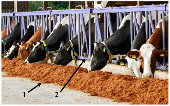
Figure 1.
Preliminary semantic segmentation Images: 1-feed, 2- frame of milking cows’ stall.
At the designing stage of the pusher robot control system, the expected trajectory of the robot motion was modeled. For autonomous positioning of the designed robot, its motion trajectory should be elementary; it moves in a straight line with minor deviations depending on the amount of feed residue on the feed table (Figure 2).
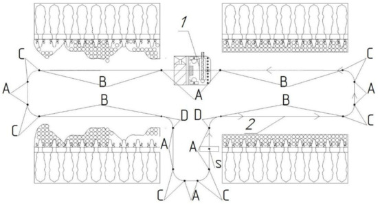
Figure 2.
Schematic diagram of the pusher robot travelling along the cattle farm. 1—pusher robot, 2—robot movement trajectory.
The robot starts travelling from the point (S) shown on the motion diagram (Figure 2); at this spot, the robot battery is charged, and the dispenser hopper is filled with feed additives.
Section (A)—the robot is moving in a straight line. At this moment, the pusher-auger and the dispenser drives are turned off; the drive of the right and left wheels operates at a constant speed.
Section (B)—the robot moves in a straight line along the feed table with slight deviations depending on the degree of spread of the feed by the animals. In the process of moving along section (B), the pusher auger rotates at a speed of 80 to 120 rpm, and the feed additives are dispensed from the dispenser hopper.
Section (C)—the robot turns to the left, so that the left wheel drive is fixed, and the right wheel drive rotates at a constant speed until the robot reaches the angle of 90°, while the drive of the dispenser and the pusher auger are disconnected.
Section (D)—the robot turns to the right so that the right wheel drive is fixed, and the left wheel drive rotates at a constant speed until the robot reaches the angle of 90°, while the drive of the dispenser and the pusher auger are disconnected.
2.2. Features of Cattle Feeding, Feed Additives and Their Ratio in the Diet
The productive qualities of cattle are maintained and increased by feeding natural, high-quality feed and adding other components of the diet. The energy value of the feed mixture can be increased by including concentrated feed, but high productivity often causes rapid deaths of animals. One of the most common opinions is that the increased productivity of dairy cows leads to the leaching of minerals (Ca, K, Na, Mg) from the animal’s body, and the farmer is often unable to identify the needs of animals in time [25].
If we consider the structure of the feeding ration, the mass fraction of Ca, K, Na, Mg supplied in the form of premixes is less than 1%. Consequently, animals may often receive less mineral supplements due to the technological features of machines that mix feed mixture components.
The developed robot is a tool for carrying out cyclic manipulations on the feed table, increasing animals’ interest in feed, and dosing energy compound feed or mineral supplements repeatedly during each feeding cycle, taking into account livestock breeding recommendations.
An installable feed additive dispenser with automatic performance control system, can provide an individual feeding mode for each group of animals.
Depending on the stage of lactation—from 15 to 30% of calcium is in a “mobile” state; it can pass from bone tissue into the blood and other tissues—it is essential to control this indicator at the peak of lactation when a large amount of minerals is released with a large volume of milk. It is also important to note that Phosphorus (P) is an antagonist of Calcium (Ca) and their ratio must equal Ca/P = 1.5 − 2/1 [26,27,28,29,30].
Phosphorus ranks second after calcium in terms of the level of content in the body. It is responsible for the formation of cell membranes and is necessary for rumen microorganisms’ regular activity. It also plays a vital role in the metabolism and transport of fats, proteins and carbohydrates. Therefore, it is necessary for the normal absorption of calcium, an active catalyst and stimulator of the effective use of feed.
Potassium (K) is a key element responsible for the reproduction of cows. Sodium (Na) provides the acid-base balance of the body and the rumen of the animal. The consumption rate is from 0.1 to 0.2% of dry matter of the daily ration Na/K = 1/2−4. When feeding cows with green mass, silage, haylage and root crops, it is necessary to introduce an increased amount of table salt into the rations than in case of the hay-concentrate feeding.
Large amounts of calcium and phosphorus in feed increase the animal’s need for magnesium (Mg). An excess of magnesium in the diet leads to increased excretion of calcium and phosphorus from the body. Its deficiency causes a slowdown in the growth of animals and a violation of their nervous and muscular activity.
Sulfur(S) helps improve the utilization of non-protein nitrogen, the digestion of fiber and starch in the rumen [30,31,32,33].
A controlled dispenser located in the robot body will provide for online manipulation of the dosage of mineral supplements and optimize the value of the animal ration.
2.3. Computer and Physical Modeling
Computer modeling involved the use of MATLAB Simulink software. Its libraries of configurable blocks, representing real-life components, such as electric motors, axis and frames, allow for the designing of an accurate robot model. The present research modeled a robot that uses two stepper motors with rigid linkage to the wheels through a reduction gear to drive, allowing a precise positioning of the robot. Also, a designed intelligent control system enabled the robot to follow the pre-configured path and react to unexpected obstacles [34].
The physical model was built on a scale of 1:1 using aluminum extrusions and equipped with stepper motors, a control and communication system, and sets of sensors for positioning. The model can provide feedback both through a wireless connection and an installed display. Also, the research team tested a binocular vision system based on an Nvidia Jetson platform. Figure 3 shows its double-camera configuration and a control board.
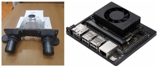
Figure 3.
Binocular vision system.
3. Results
3.1. Results of an Artificial Experiment (Kinematic Model and Dynamic Model of the Robot)
At the stage of selecting the element base of the pusher robot, kinematic and dynamic analysis was carried out, taking into account the robot’s mass, the indicators of the acting forces in the process of motion, according to the analysis scheme presented in Figure 4.
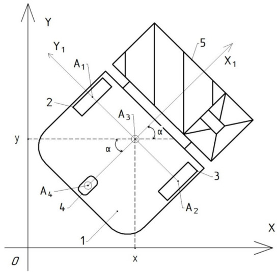
Figure 4.
Design scheme describing the robot motion kinematics. 1, mobile platform; 2, drive wheel; 3, drive wheel; 4, support wheels; 5, pushing auger. —the fulcrum of the left driving wheel, —the fulcrum of the right driving wheel, —the center of mass of the robot, —the point of support of the driven wheel.
The robot is a mobile platform with two driving wheels and one driven one. The driving wheels are located on the same axle. The center of each wheel is designated by the letter and , respectively, with . The robot moves on a surface that is located in the Oxy plane.
The robot’s gravity center is presumably located at point, belonging to the coordinate system. Attachments are mounted on the robot body, which are designed to push the distributed feed.
The axis is rigidly fixed to the robot and is the vertical of the movable base. The rotation angle of the base vertical line about the Ox axis is denoted by α, and the angular velocity of the platform is .
The position of the mobile robot relative to the Oxy world reference system is indicated by point with coordinates (x, y).
The motion speed of a point along the Ox and Oy coordinates is described by Equations (1) and (2), respectively:
The following equality holds true: = .
The speed of point is determined by Equation (3):
The rotation angles of the driving wheels (centered at points and , respectively) relative to the horizontal planes are , and , then the angular velocity will equal and , respectively.
The motion speed of point is determined by Equation (4)
where R—the radius of the driving wheels.
The system of motion equations of the robotic installation will take the form:
Equations for solving inverse kinematics:
To describe the dynamics of a mobile robot, we use the Appel equation, which can be presented in a matrix form as follows:
Here, the operation of differentiating the scalar Appel function S taking into account the vector of pseudo-accelerations is performed; is the vector of pseudo-generalized forces. In this case, the components of the vector of pseudo-generalized forces are determined with the Equations:
where , are the moments developed by the stepper electric drives of the wheels.
3.2. Control System Design
Figure 5 shows a mathematical model of a pusher robot, obtained using the Simulink Matlab library.
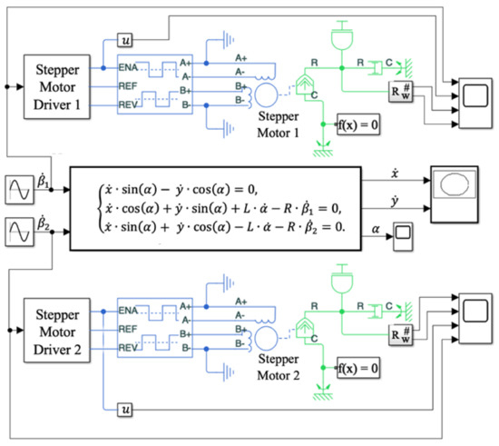
Figure 5.
Mathematical model of the feed pusher robot.
The central block of the mathematical model is the robot’s kinematic model, the input of which receives the angular velocities of the driving wheels and .
The aforementioned signals are also fed to the stepper motor controllers of the driving wheels, which generate control actions to operate them. Within the framework of the dynamic model, ready-made control blocks for stepper motors of the Simulink library are used. The motor control logic contained in the Stepper Motor Driver 1–2 blocks is a controller. The developed model makes it possible to change the geometric data of the mobile platform of the robot and design the transient processes of the dynamic and kinematic structural components.
Figure 6 shows a functional control diagram of the robot’s physical model described mathematically.
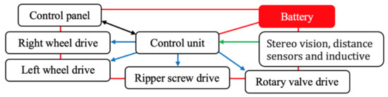
Figure 6.
Functional diagram of the pusher robot.
The control circuit includes a microprocessor-based controller that processes and analyzes input telemetry from inductive sensors and a binocular vision system. In turn, the control is carried out by the output signals of the mobile robotic system. All elements are battery-powered; visual control is carried out using the display on the remote control.
The system of automatic control of the robot’s motion implies determining the deviation from a given motion trajectory by signals from two inductive sensors and the binocular vision unit, and analyzing control pulses based on fuzzy-rules logical inference. The authors have established that stereo vision increases predictive properties of the sensor system. The structural diagram of the automatic robot motion control system is shown in Figure 7.
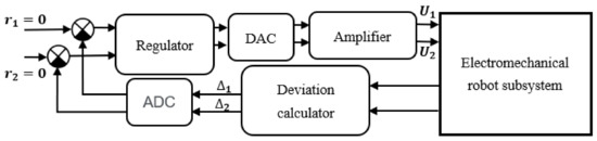
Figure 7.
Structural diagram of the automatic robot’s motion control system.
3.3. Simulations (Modeling)
The overview part of this paper analyses the planned motion trajectory of the pusher robot around a dairy farm. Figure 8 shows the scheduled motion trajectory. The mobile robot made a U-turn during the motion starting since it was oriented in the opposite direction. The different lines represent the trajectories of the other wheels of the platform. The mobile platform’s algorithm is designed so that the system tends to position the robot’s center of gravity at a given point.
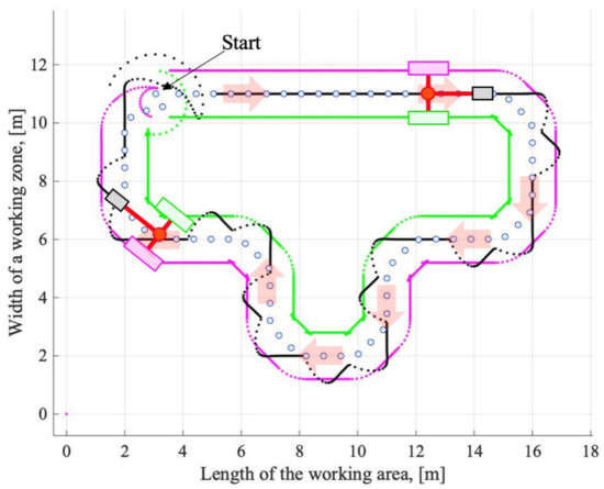
Figure 8.
The wheel trajectory of the mobile robot.
The stepper motor shaft rotates, performing discrete movements. This is achieved through a smart rotor shape and two/four windings. As a result, by alternating the voltage direction in the windings, it is possible to make the rotor have alternatively fixed values turns. The developed mathematical model makes it possible to track the engine operation dynamics and the control action pattern.
Figure 9 shows the transient processes of the rotation angle of the stepper motor shaft (a) and the control action received by the stepper motor controllers (b). Evident from the characteristics, the control action turns the engine rotor rigidly fixed to its shaft, thereby making it rotate. Nevertheless, the system has an inherent overshoot during positioning, observed in the transient response (a).
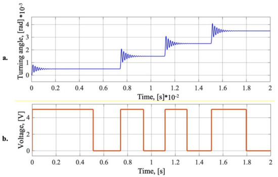
Figure 9.
Time charts, (a) transient process of the rotation angle of a stepper motor shaft, (b) transient process of the control action on stepper motor controllers.
The way of implementing the control system for the pusher robot is shown in Figure 10. The control unit consists of two boards, one of which is a driver for controlling the electric motor; the second board processes incoming signals from the sensors of the positioning system and the console to change the parameters of autonomous operation.
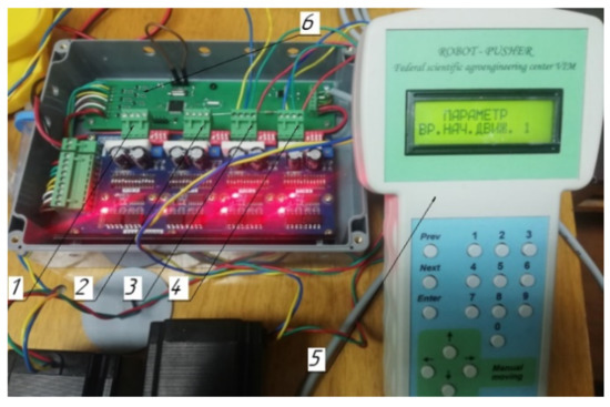
Figure 10.
Time Elements of the control system of the pusher robot; 1, output to the left wheel drive; 2, output to the right wheel drive; 3, output to the pusher auger drive; 4, output to the dispenser drive; 5, control panel for changing the parameters of automatic operation; 6, input signal processing board.
In most general industrial wheeled robots, GPS or Lidar systems are used for positioning. Still, the GPS inside the farm building does not always provide the necessary travelling accuracy, so Lidar is an expensive tool and difficult to program.
Therefore, according to the results of analyzing the positioning systems, it is reasonable to use inductive sensors installed in the robot’s base on both sides of a predetermined trajectory. This can be implemented in the form of a metal strip or cable capable of reflecting a signal mounted at the level of the feeding table surface, along which the robot moves.
The designed system can also position the robot according to the distance sensor to the objects standing aside from the trajectory. The distance sensor also allows for the determining of the necessary deviation from the trajectory, depending on the amount of feed residues on the feed table.
The distance sensor is used in this system as additional feedback on the mobile base position, serving as a verified element of the binocular vision system operation. The rigid mounting of the binocular vision system is a must as its signal forms the robot’s trajectory. In Figure 11, fodder 1 is segmented using an intelligent algorithm. Transition characteristic 3 shows the volume of feed distributed along its trajectory and detected while the robot is travelling. Due to the rigid mounting of the distance sensor on the body and the rectilinear motion of the robot, the trajectory of a fixation signal sent from the distance sensor also takes a linear form (No.3 in the figure).
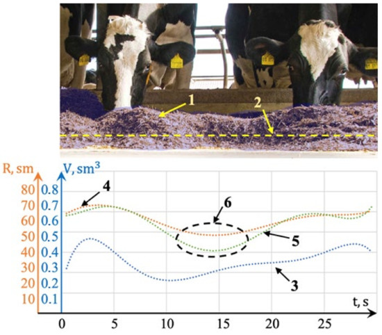
Figure 11.
Feed detection and data verification system for the binocular vision system and distance sensor; 1, feed detection zone, 2, trajectory signal fixation received from the distance sensor, 3, characteristics of the feed volume after scanning the table in the direction of movement of the robot, 4, the trajectory of movement set by the control signal of the distance sensor, 5, the trajectory of movement set by the control signal of binary vision, 6, the area of data inconsistency.
Transient characteristics 4 and 5 are the signal from the distance sensor and the result of the linear interpretation of the data from the binocular vision system, respectively. The linear interpretation of the data in the intelligent algorithm is an array of points that lie on the surveyed distance sensor path but are generated from the data acquired from the binocular vision system. The presence of short-term discrepancies (shown in Figure 11, 6) indicates the milking animal’s activity during feeding at the moment of feed dispensing. The data were obtained from the binocular vision system or a distance sensor. If discrepancies are not short-term, the operator will receive a message to check the attachment of the distance sensor and the binocular vision system.
Figure 12 shows the physical model of the pusher robot. Some parts of the robot (the pusher auger, the feed additives dispenser) were made in the laboratory using 3-D printing technology.
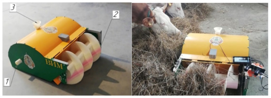
Figure 12.
Physical analogue of a robot pusher; 1, outlet of the feed additives dispenser; 2, pusher auger; 3, filler with a closer.
4. Discussion
The study examined how effectively the simulated and developed wheel drive system and the automatic positioning system interact with each other. The criterion for evaluating the effectiveness was the deviation of the robot’s center of mass from the given trajectory of motion.
Figure 13 shows simulated trajectories of the x and y coordinates of the gravity center of the mobile robot. The dashed lines represent the specified trajectories, the solid lines represent the results of modeling the developed intelligent algorithm. It is apparent that the maximum mismatch error between the set value and the result of modeling the positioning of the mass center of the movable platform reaches σ ≈ 30 mm.
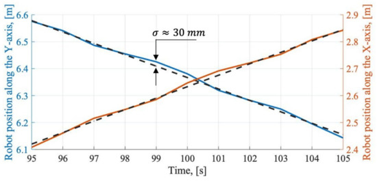
Figure 13.
Trajectories of x and y coordinates of the mobile robot’s gravity center.
The main factor influencing this error is the accuracy of the feedback sensors and the interaction quality of the kinematic pairs.
When conducting field tests, in one case, inductive sensors mounted in the inner part of the robot body and connected to the control board were used as a feedback system. In turn, a metal strip mounted on the feed table surface was used to guide the motion trajectory. An error has been minimized due to the reliability of the communication system.
When a binocular vision system served as a key tool for controlling the navigation system, there was a positioning error of the robot of up to 100 mm, since the system is sensitive to the movements of animals located at the fence of the feeding table. In this regard, the distance sensor telemetry provides the primary feedback for disorienting the robot on the plane (going off track).
Thus, when using stepper motors and rigidly articulated drive wheels with an electric drive, it was possible to minimize the inaccuracy of the operation of kinematic pairs. In turn, the positioning systems must be made reliable since the robot may be out of animals’ reach during feed dispensing, contributing to the inaccessibility of the distributed feed.
5. Conclusions
- The considered mathematical model of the mobile feed pusher presents a sufficient set of tools that can serve as the basis for designing and improving the robot in the engineering analysis and the selection of actuators.
- The use of the designed robot can significantly facilitate the farmer’s work by carrying out labor-intensive operations to push feed on the feed table without human intervention.
- When using inductive sensors and the metal strip contour, the minor positioning error of the wheeled robot was compared with the binocular vision system. The animals present at the feed table may cause interference in the binocular vision system and destabilize the control algorithm.
Author Contributions
Conceptualization and methodology, D.Y.P. and D.V.S.; validation, E.A.N.; formal analysis, D.V.S. and E.A.N.; investigation and resources, E.A.N. and I.A.K.; writing—original draft preparation, D.Y.P. and E.A.N.; writing—review and editing, I.A.K., visualization, D.V.S.; supervision and funding acquisition, D.Y.P.; project administration, D.V.S. All authors have read and agreed to the published version of the manuscript.
Funding
This work was supported by the Ministry of Education and Science of the Russian Federation in the framework of the State Assignment of “Federal Scientific Agroengineering Center VIM” (task No. 0581-2021-0009).
Institutional Review Board Statement
Not applicable.
Informed Consent Statement
Informed consent was obtained from all subjects involved in the study.
Conflicts of Interest
The authors declare no conflict of interest. The funders had no role in the design of the study; in the collection, analyses, or interpretation of data; in the writing of the manuscript, or in the decision to publish the results.
References
- Pavkin, D.Y.; Nikitin, E.A.; Zobov, V.A. Robotic System for Maintenance of Feed Table for Livestock Complexes. Agric. Mach. Technol. 2020, 14, 33–38. [Google Scholar] [CrossRef]
- Nabokov, V.I.; Novopashin, L.A.; Denyozhko, L.V.; Sadov, A.A.; Ziablitckaia, N.V.; Volkova, S.A.; Speshilova, I.V. Applications of feed pusher robots on cattle farmings and its economic efficiency. Int. Trans. J. Eng. Manag. Appl. Sci. Technol. 2020, 14, 11. [Google Scholar] [CrossRef]
- Oberschätzl, R.; Haidn, B.; Neiber, J.; Neser, S. Automatic feeding systems for cattle—A study of the energy consumption of the techniques. In Proceedings of the Environmentally Friendly Agriculture and Forestry for Future Generations XXXVI CIOSTA CIGR V Conference, Saint Petersburg, Russia, 26–28 May 2015. [Google Scholar]
- Buza, M.; Holden, L.; White, R.; Ishler, V. Evaluating the effect of ration composition on income over feed cost and milk yield. J. Dairy Sci. 2014, 97, 3073–3080. [Google Scholar] [CrossRef] [PubMed] [Green Version]
- Albright, J. Feeding Behavior of Dairy Cattle. J. Dairy Sci. 1993, 76, 485–498. [Google Scholar] [CrossRef]
- Harper, M.; Oh, J.; Giallongo, F.; Lopes, J.; Weeks, H.; Faugeron, J.; Hristov, A. Short communication: Preference for flavored concentrate premixes by dairy cows. J. Dairy Sci. 2016, 99, 6585–6589. [Google Scholar] [CrossRef] [PubMed]
- Miller-Cushon, E.; Devries, T. Feed sorting in dairy cattle: Causes, consequences, and management. J. Dairy Sci. 2017, 100, 4172–4183. [Google Scholar] [CrossRef]
- Bach, A.; Iglesias, C.; Busto, I. Technical Note: A Computerized System for Monitoring Feeding Behavior and Individual Feed Intake of Dairy Cattle. J. Dairy Sci. 2004, 87, 4207–4209. [Google Scholar] [CrossRef]
- Wolf, C. Understanding the milk-to-feed price ratio as a proxy for dairy farm profitability. J. Dairy Sci. 2010, 93, 4942–4948. [Google Scholar] [CrossRef]
- Deniz, N.N.; Chelotti, J.O.; Galli, J.R.; Planisich, A.M.; Larripa, M.J.; Rufiner, H.L.; Giovanini, L.L. Embedded system for real-time monitoring of foraging behavior of grazing cattle using acoustic signals. Comput. Electron. Agric. 2017, 138, 167–174. [Google Scholar] [CrossRef]
- De Berg, M.; Gerrits, D.H.P. Computing Push Plans For Disk-Shaped Robots. Int. J. Comput. Geom. Appl. 2013, 23, 29–48. [Google Scholar] [CrossRef] [Green Version]
- Rudolfs, R. Agris Nikitenko Development of Free-Flowing Pile Pushing Algorithm for Autonomous Mobile Feed-Pushing Robots in Cattle Farms. Eng. Rural. Dev. 2018, 23, 958–963. [Google Scholar] [CrossRef]
- Sekiguchi, S.; Yorozu, A.; Kuno, K.; Okada, M.; Watanabe, Y.; Takahashi, M. Human-friendly control system design for two-wheeled service robot with optimal control approach. Robot. Auton. Syst. 2020, 131, 103562. [Google Scholar] [CrossRef]
- Fonseca, L.M.; Savi, M.A. Nonlinear dynamics of an autonomous robot with deformable origami wheels. Int. J. Non-Linear Mech. 2020, 125, 103533. [Google Scholar] [CrossRef]
- Tsai, S.-H.; Kao, L.-H.; Lin, H.-Y.; Lin, T.-C.; Song, Y.-L.; Chang, L.-M. A Sensor Fusion Based Nonholonomic Wheeled Mobile Robot for Tracking Control. Sensors 2020, 20, 7055. [Google Scholar] [CrossRef] [PubMed]
- De León, J.; Cebolla, R.; Barrientos, A. A Sensor Fusion Method for Pose Estimation of C-Legged Robots. Sensors 2020, 20, 6741. [Google Scholar] [CrossRef]
- Wang, F.; Qin, Y.; Guo, F.; Ren, B.; Yeow, J.T.W. Adaptive Visually Servoed Tracking Control for Wheeled Mobile Robot with Uncertain Model Parameters in Complex Environment. Complexity 2020, 2020, 8836468. [Google Scholar] [CrossRef]
- Xin, L.; Wang, Q.; She, J.; Li, Y. Robust adaptive tracking control of wheeled mobile robot. Robot. Auton. Syst. 2016, 78, 36–48. [Google Scholar] [CrossRef]
- Wu, H.-M.; Karkoub, M. Hierarchical Fuzzy Sliding-Mode Adaptive Control for the Trajectory Tracking of Differential-Driven Mobile Robots. Int. J. Fuzzy Syst. 2018, 21, 33–49. [Google Scholar] [CrossRef]
- Wu, X.; Jin, P.; Zou, T.; Qi, Z.; Xiao, H.; Lou, P. Backstepping Trajectory Tracking Based on Fuzzy Sliding Mode Control for Differential Mobile Robots. J. Intell. Robot. Syst. 2019, 96, 109–121. [Google Scholar] [CrossRef]
- Shtessel, Y.; Taleb, M.; Plestan, F. A novel adaptive-gain supertwisting sliding mode controller: Methodology and application. Automatica 2012, 48, 759–769. [Google Scholar] [CrossRef]
- Khalil, H.K.; Praly, L. High-gain observers in nonlinear feedback control. Int. J. Robust Nonlinear Control 2014, 24, 993–1015. [Google Scholar] [CrossRef]
- Jin, X. Fault-tolerant iterative learning control for mobile robots non-repetitive trajectory tracking with output constraints. Automatica 2018, 94, 63–71. [Google Scholar] [CrossRef]
- Boukens, M.; Boukabou, A.; Chadli, M. Robust adaptive neural network-based trajectory tracking control approach for nonholonomic electrically driven mobile robots. Robot. Auton. Syst. 2017, 92, 30–40. [Google Scholar] [CrossRef]
- Bloch, V.; Levit, H.; Halachmi, I. Assessing the potential of photogrammetry to monitor feed intake of dairy cows. J. Dairy Res. 2019, 86, 34–39. [Google Scholar] [CrossRef] [PubMed]
- Halachmi, I.; Ben Meir, Y.; Miron, J.; Maltz, E. Feeding behavior improves prediction of dairy cow voluntary feed intake but cannot serve as the sole indicator. Animal 2016, 10, 1501–1506. [Google Scholar] [CrossRef]
- Bargo, F.; Muller, L.; Delahoy, J.; Cassidy, T. Milk Response to Concentrate Supplementation of High Producing Dairy Cows Grazing at Two Pasture Allowances. J. Dairy Sci. 2002, 85, 1777–1792. [Google Scholar] [CrossRef] [Green Version]
- Bach, A.; Cabrera, V. Robotic milking: Feeding strategies and economic returns. J. Dairy Sci. 2017, 9, 7720–7728. [Google Scholar] [CrossRef] [PubMed] [Green Version]
- Schneider, L.; Volkmann, N.; Kemper, N.; Spindler, B. Feeding Behavior of Fattening Bulls Fed Six Times per Day Using an Automatic Feeding System. Front. Vet. Sci. 2020, 7, 43. [Google Scholar] [CrossRef] [Green Version]
- Halachmi, I.; Edan, Y.; Maltz, E.; Peiper, U.; Moallem, U.; Brukental, I. A real-time control system for individual dairy cow food intake. Comput. Electron. Agric. 1998, 20, 131–144. [Google Scholar] [CrossRef]
- Bach, A.; Valls, N.; Solans, A.; Torrent, T. Associations between Nondietary Factors and Dairy Herd Performance. J. Dairy Sci. 2008, 91, 3259–3267. [Google Scholar] [CrossRef] [Green Version]
- Pezzuolo, A.; Chiumenti, A.; Sartori, L.; Da Borso, F. Automatic feeding system: Evaluation of energy consumption and labour requirement in north-east italy dairy farm. In Proceedings of the 15th International Scientific Conference: Engineering for Rural Development, Jelgava, Latvia, 25–27 May 2016; pp. 882–887. [Google Scholar]
- Reger, M.; Bernhardt, H.; Stumpenhausen, J. Navigation and personal protection in automatic feeding systems. Actual Tasks Agric. Eng. 2017, 45, 523–530. [Google Scholar]
- Grechin, G.; Shilin, D.; Zayceva, A. Development of an Algorithm for Searching the Optimal Trajectory of the Object in the Conditions of Given Restrictions. In Proceedings of the 2020 V International Conference on Information Technologies in Engineering Education (Inforino), Moscow, Russia, 14–17 April 2020; pp. 1–4. [Google Scholar]
Publisher’s Note: MDPI stays neutral with regard to jurisdictional claims in published maps and institutional affiliations. |
© 2021 by the authors. Licensee MDPI, Basel, Switzerland. This article is an open access article distributed under the terms and conditions of the Creative Commons Attribution (CC BY) license (https://creativecommons.org/licenses/by/4.0/).