An Attention-Based Convolutional Neural Network for Acute Lymphoblastic Leukemia Classification

Abstract

Leukemia is a kind of blood cancer that influences people of all ages and is one of the leading causes of death worldwide. Acute lymphoblastic leukemia (ALL) is the most widely recognized type of leukemia found in the bone marrow of the human body. Traditional disease diagnostic techniques like blood and bone marrow examinations are slow and painful, resulting in the demand for non-invasive and fast methods. This work presents a non-invasive, convolutional neural network (CNN) based approach that utilizes medical images to perform the diagnosis task. The proposed solution consisting of a CNN-based model uses an attention module called Efficient Channel Attention (ECA) with the visual geometry group from oxford (VGG16) to extract better quality deep features from the image dataset, leading to better feature representation and better classification results. The proposed method shows that the ECA module helps to overcome morphological similarities between ALL cancer and healthy cell images. Various augmentation techniques are also employed to increase the quality and quantity of training data. We used the classification of normal vs. malignant cells (C-NMC) dataset and divided it into seven folds based on subject-level variability, which is usually ignored in previous methods. Experimental results show that our proposed CNN model can successfully extract deep features and achieved an accuracy of 91.1%. The obtained findings show that the proposed method may be utilized to diagnose ALL and would help pathologists.

1. Introduction

Acute lymphoblastic leukemia, generally known as ALL, is a type of blood cancer that usually begins in the bone marrow where the blood cells are formed. It is the type of cancer that is associated with white blood cells (WBC). Based on the age of the disease, leukemia is divided into four main types: chronic lymphocytic leukemia (CLL), chronic myeloid leukemia (CML), acute myelogenous leukemia (AML), and acute lymphoblastic leukemia (ALL) [1,2]. In acute leukemia, the abnormal cells grow and spread rapidly and require immediate treatment, while chronic leukemia is hard to detect in its early stages. As a result, the blood cannot perform its normal function, making the immune system more susceptible. Moreover, in ALL bone marrow cannot produce healthy platelets and red blood cells, making most parts of the body vulnerable [3].

In ALL, bone marrow generates a large quantity of abnormal WBC. These WBC can stream into the blood and harm different parts of the body like the spleen, brain, kidney, and liver, which can lead to other dangerous types of cancer. Since ALL can spread quickly throughout the body, sometimes it can cause deaths if not treated or diagnosed in the early stage. According to the key statistics about ALL, in 2021 more than 5690 cases of ALL are identified in the United States only [4] and out of which more than 1550 people are anticipated to die including both youngsters and adults. If leukemia, and especially ALL is diagnosed in its early stages, it is easily curable. The symptoms of leukemia are similar to other diseases like anemia, joint pain, fever, weakness, and bone pain, which is why the diagnosis of leukemia sometimes becomes difficult.

There are a number of invasive methods which are usually used by hematologists to diagnose the disease. Generally, a biopsy is done which is an invasive method that is done by conducting tests on blood, bone marrow or spinal fluid [5]. These methods are painful, costly, and time-consuming. In these checkups, the medical specialist examines if the quantity of WBCs is sufficiently high and there are other relevant physical observations then it is highly likely the presence of ALL. These manual and expert-specific methods are also prone to error as the results of such methods are highly dependent on the knowledge and skills of the expert conducting the analysis [6]. To avoid the complexities involved with such invasive methods, and to provide faster, safe, and cost-effective solutions, medical image analysis-based techniques are employed. Image processing and computer vision-based methods are easy to generalize and eliminate the error of human factor.

The image-based analysis can easily be done by radiologists. Such methods can provide benefit in a way that these are non-invasive however they do suffer from the same issues as invasive methods. The manual analysis by radiologists becomes burdensome, error-prone, and tremendously tedious when human experts are required to analyze the large datasets consisting of hundreds and thousands of medical images. Inherent overlapping features like morphology and texture in medical, especially histopathology images make the task harder. This fact is shown clearly in Figure 1, where images of ALL cancer and healthy cells are given. One can observe that these leukocytes are difficult to detect and classify due to their high intraclass homogeneity and low interclass separability. Consequently, developing accurate and reliable methodologies for leukemia recognition is important for timely diagnosis and early treatment. However, in general, ALL cancer cells differ from healthy cells on the basis of various factors including morphology, cell size, shape, and texture [7]. A computational classifier can use any of these distinguishing features to distinguish ALL cancer and healthy cell images.

To remove the aforementioned issues associated with invasiveness and human experts, a fully automated solution based on convolutional neural networks is proposed in this work. The features associated with the dataset play a vital role for statistical, computational learners. Therefore, we trained the CNN model from scratch instead of the transfer learning paradigm used in other work [10,13,14,15]. Although the cell image features may differ significantly from natural images, a network trained from scratch on cell images may converge to a better solution. To improve the quality and quantity of available datasets, a number of preprocessing methods are used including data augmentation to improve the generalizability and class balancing to avoid overfitting or bias incorporation due to dataset. In this work, we proposed an attention-based CNN to address the task of categorization of ALL and healthy cell images. The designed deep learning model is trained from scratch on the preprocessed dataset to obtain parameter values that are most relevant and provide better convergence for the network.

2. Related Work

2.1. Conventional Machine Learning Algorithms

Joshi et al. [16] developed a method for the segmentation and classification of white blood cells. For the preprocessing of microscopic blood images, they used histogram equalization and contrast enhancement. In addition, to extract white blood cells, they used the Otsu thresholding segmentation. The extracted features were given to K nearest neighbor (KNN) clustering to categorize the blood images into normal and blast cells. The proposed method was tested on 108 images of peripheral blood smears from a publicly available dataset.

Another unsupervised segmentation method was developed by Mohapatra et al. [17] based on color scheme clustering for the classification of leukemia. A two-stage color segmentation approach based on fuzzy logic was used to differentiate leukocytes from other constituents of the blood. The authors extracted the features like the fractal dimension, shape, texture, and the signature of the contour. Their proposed method used 270 images for the classification of ALL. MoradiAmin et al. [7] proposed an enhanced method for ALL recognition. In this method, they utilized fuzzy c-means clustering for the segmentation of lymphocytes. After feature extraction, they used principal component analysis (PCA) to reduce the features and fed them to the support vector machine (SVM) classifier to distinguish between normal and blast cells. They conducted their experiment on 958 images.

Putzu et al. [18] proposed a method that isolates the leukocytes from a microscopic image and further distinguishes the nuclei and cytoplasm from the leukocytes. They trained different classification models and extracted shape, color, and texture features to determine which model is best suitable for leukemia classification. They used 368 images and tested several classifiers for classification purposes. Based on the classification accuracy they found that SVM with a Gaussian radial basis kernel outperforms other classifiers. Singhal et al. [19] developed an automatic detection algorithm for ALL based on local binary pattern (LBP) and geometric texture features. Their proposed model used a small dataset composed of 368 images for features extraction and these features are then fed to SVM for binary classification. Patel et al. [20] proposed a method for automatic detection of leukemia from 108 microscopic images. They applied some filtering techniques to extract the important parts from images and then K-means clustering was used to produce the binary clusters. For classification purposes, they used an SVM classifier to distinguish between healthy and malignant cells. Karthikeyan et al. [21] came up with a novel idea for leukemia detection using stained blood microscopic images. They used the median filter and histogram equalization for image preprocessing. For segmentation purposes, they used fuzzy c-means and SVM to classify the leukemia cells into normal and malignant classes. They used 19 microscopic images for leukemia cancer classification. Another segmentation and classification method proposed by Mohammad et al. [22] involves the transformation of grayscale images to color space YCbCr. Then they computed the Gaussian distribution on each color and calculated a number of features like texture, scale, and morphology. These features are then given as input to the random forest classifier. They used a dataset of 105 images to train their model for WBCs classification.

A significant drawback of these methods is they used small datasets to classify ALL cell images. A classifier trained on a small dataset is more vulnerable to overfitting and may not give an optimal result. The used datasets in the literature vary from 19 to 958 images. Another drawback is that these researchers used conventional machine learning algorithms (SVM, KNN, K-means clustering), which use handcrafted features that may not be an optimal set of features for classification. All these drawbacks can limit the final performance. Thus, there is still a need to devise high-performance algorithms based on a larger dataset and extract features using an automated technique to diagnose ALL with better accuracy.

2.2. Deep Learning-Based Methods

With the emergence of deep neural networks, we can achieve better performance in computer vision. A deep neural network can automatically extract task-specific features using two-dimensional convolutional filters to overcome the problem of predefined features. Deep neural networks are widely utilized in the field of computer vision, especially for medical image analysis, such as disease classification [23], localization [24], detection [25], registration [26], and segmentation [27,28]. However, the performance of a deep neural network depends on the size of the dataset, but unfortunately, it is hard to get a larger dataset for medical image analysis. In order to deal with small dataset transfer, learning strategy and data augmentation can be used to overcome the problem of the limited dataset. Rehman et al. [29] used a pre-trained AlexNet and fine-tuning to identify ALL subtypes on a private dataset composed of 330 images. Shafique et al. [30] proposed a deep CNN to classify all four subtypes of leukemia. To avoid training from scratch they used a pre-trained AlexNet to perform binary classification on 368 images. A classification model focused on both transfer learning and deep learning was proposed by Habibzadeh et al. [31] for WBC classification. The proposed approach began with preprocessing of the dataset and then employed transfer learning for feature extraction. Finally, the Inception and ResNet were used to perform WBCs classification. Their proposed model used 352 images for WBC classification. Ahmad et al. [32] proposed a CNN model that recognizes all subtypes of leukemia. Initially, they used 903 images for classification of ALL subtypes. They also used seven distinct data augmentation techniques to enhance the dataset size. In comparison to CNN, they also investigated other machine learning algorithms like decision tree (DT), SVM, Naïve Bayes, and KNN and found that CNN outperforms all other methods. Wang et al. [33] used SVM to identify spatial features and then suggested a neural network with marker-based learning vector quantization to detect and classify ALL cells. They used 24 samples (16 out of 27 ALL patients and 8 normal samples with no clinical history of leukemia) to train their proposed method for ALL diagnosis. Pansombut et al. [34] proposed a new method to identify ALL and its subtypes using a CNN network called ConVNet. They evaluated their model with other machine learning algorithms such as SVM, multilayer perceptron (MLP) and random forest. They used two types of datasets, one for ConVNet and the other for feature extraction. The overall dataset consists of 363 images.

Again, here is the problem of a limited number of images as many researchers used a tiny dataset consisting of 24 to 903 images. The performance results of such a small dataset cannot be considered an optimal performance indicator for medical image analysis. On the other hand, classification becomes extremely difficult when dealing with small datasets, which results in an incorrect and biased classification model [22]. In addition, using pre-trained models for classification needs to adjust the input image’s size according to the predefined input shape of the networks, which can alter the morphology of ALL cell images [35]. It is difficult to classify ALL cell images because these leukocytes are challenging to detect due to their high intraclass homogeneity and low interclass separability. Furthermore, they used transfer learning or fine-tuning of deep neural networks for ALL classification. A model trained on non-medical images and used for medical image classification may not achieve optimal results because the cell image features may differ significantly from natural images. A model trained from scratch on cell images may converge to a better solution.

Currently some researchers used a larger dataset for the classification of ALL. Kasani et al. [36] proposed an aggregated-based deep learning-based model for the classification of ALL. They used fine-tuning and transfer learning to propose an ensemble model based on VGG19 and NasNetLarge architecture. Kassani et al. [37] proposed a hybrid model based on VGG16 and MobileNet for the classification of ALL cell images. Global average pooling (GAP) was used between VGG16 and MobileNet to extract high-level features from ALL cell images. LeukoNet was proposed by Mourya et al. [38] for the classification of ALL cell images. The proposed model combines the discrete cosine transform (DCT) domain features extracted using CNN with the optical density (OD) space features to build an effective classifier. Although these researchers used the C-NMC 2019 dataset composed of more than 10,000 images, but they did not segregate the training data based on subject-level variability. Instead, the classifier was trained by combining all of the subject’s data into healthy and cancer classes. Because subject-specific features help in class discrimination, this pooling can restrict the classifier’s performance. As a result, a practical classifier would require training on data from certain subjects and testing using data from entirely unknown subjects. In this paper we used the C-NMC 2019 dataset for the diagnosis of ALL. The cell images in the C-NMC dataset are selected carefully based on subject-level variability. In order to get more robust results, we split the dataset into seven-fold cross-validation so that no two splits overlap in terms of subject data. This strategy also ensures that none of the cell images of a subject used in training were used to test the classifier. In comparison to other ALL datasets such as the ispat general hospital (IGH) [17], ALL image database for image processing (ALL-IDB) [39], medical image and signal processing research center (MISP) [22], and American society of hematology (ASH) [32], the C-NMC 2019 dataset has a substantially more significant number of images, which can aid in the development of a robust and scalable ALL diagnostic classifier. Our proposed simple model uses an attention module to refine features more and overcome the problem of morphological similarity bringing more reliability to the results and thus classifying the images as healthy or not. To the best of our knowledge, we are the first to use the attention module with a CNN model for ALL classification.

3. Materials and Methods

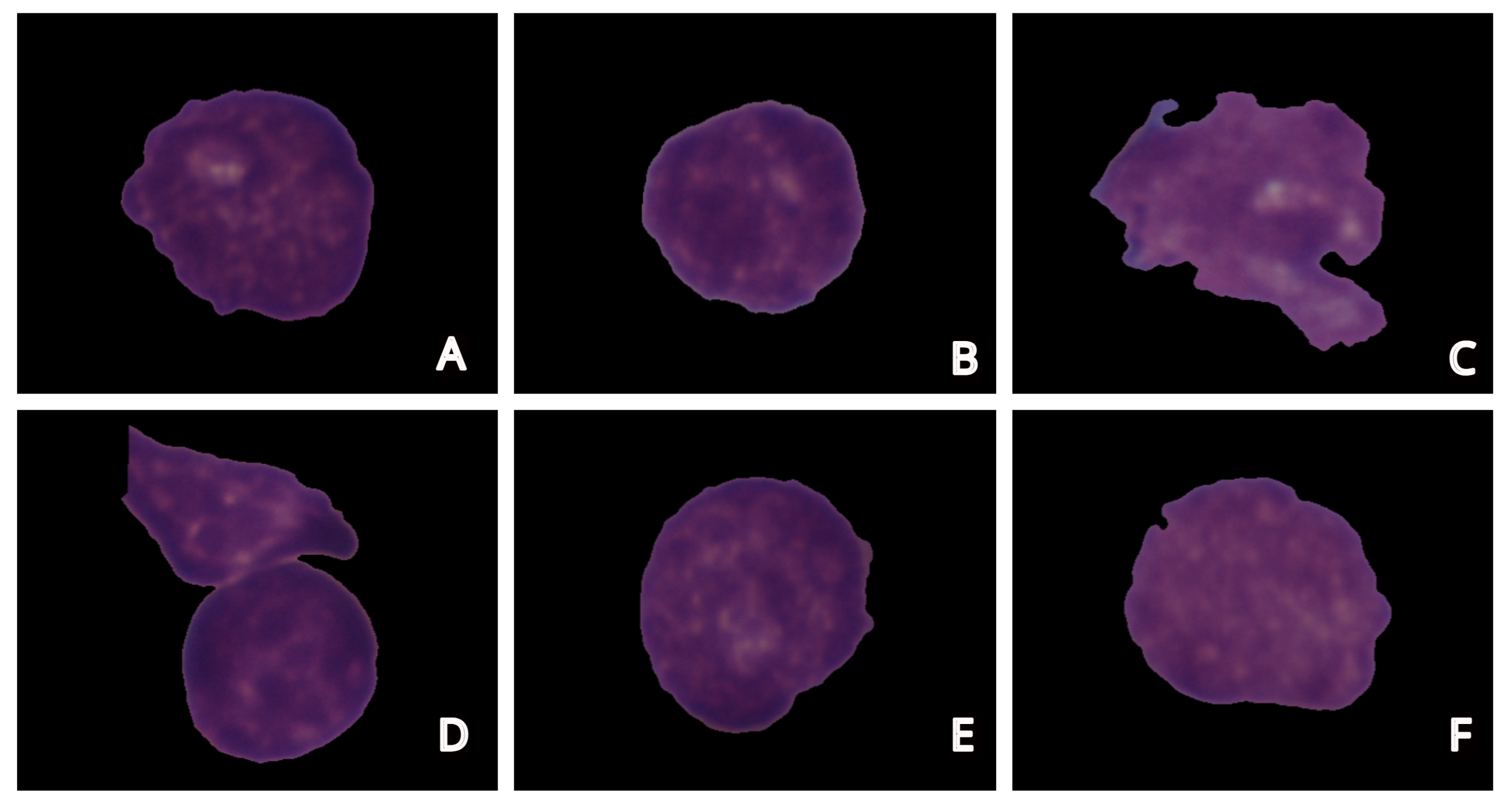
3.1. Dataset Description

We have used the publicly available dataset C-NMC 2019. The dataset is released by the cancer imaging archive (TCIA) for the ALL challenge competition. The objective of this competition is to create a computer-aided design (CAD) system to differentiate the normal cells from the leukemic blast (malignant cells) in microscopic images of blood clotting. Both training and test images have been processed to 24-bit RGB format with a consistent resolution of 450 × 450 pixels. Errors in lighting, uneven staining, and image noise have been resolved using the methods given by [11,12]. The images in this dataset were labeled as normal or malignant by an experienced oncologist. The dataset consists of 10,661 single cell images collected from 76 individual subjects, whereas 7272 images were taken from 47 patients having ALL, and the rest 3389 were taken from 26 healthy subjects. The C-NMC dataset includes a considerably large number of images that can help in designing a robust diagnostic ALL classifier. In our experiment, the dataset is divided into 7 folds based on subject-level variability as shown in

Table 1. The test and training data for each class is 7-fold. Folds 1–6 represents the training data. All cell images belonging to the same subject are placed in the same fold and not a single fold includes cell image from the same subject.

		Cancer Cell Images
Fold	No. of Subjects	No. of Images
1	8	1119
2	7	1100
3	4	1200
4	7	1218
5	8	1203
6	7	1209
Total	41	7049
		Normal Cell Images
Fold	No. of Subjects	No. of Images
1	3	562
2	4	473
3	4	538
4	3	541
5	3	524
6	3	538
Total	20	3176
		Testing Data
Class	Subjects	No. of Images
Healthy	6	213
Cancer	6	223
Total	12	436

. To avoid overfitting and to make the dataset balanced, we applied different data augmentation techniques.

3.2. Image Preprocessing

We first resized the input images into 224 × 224 as VGG16 takes an input image of size 224 × 224. Secondly, we normalized the input images by subtracting the channel-wise mean red, green, and blue (RGB) values of all images in the training set and dividing the images with standard deviation [40].

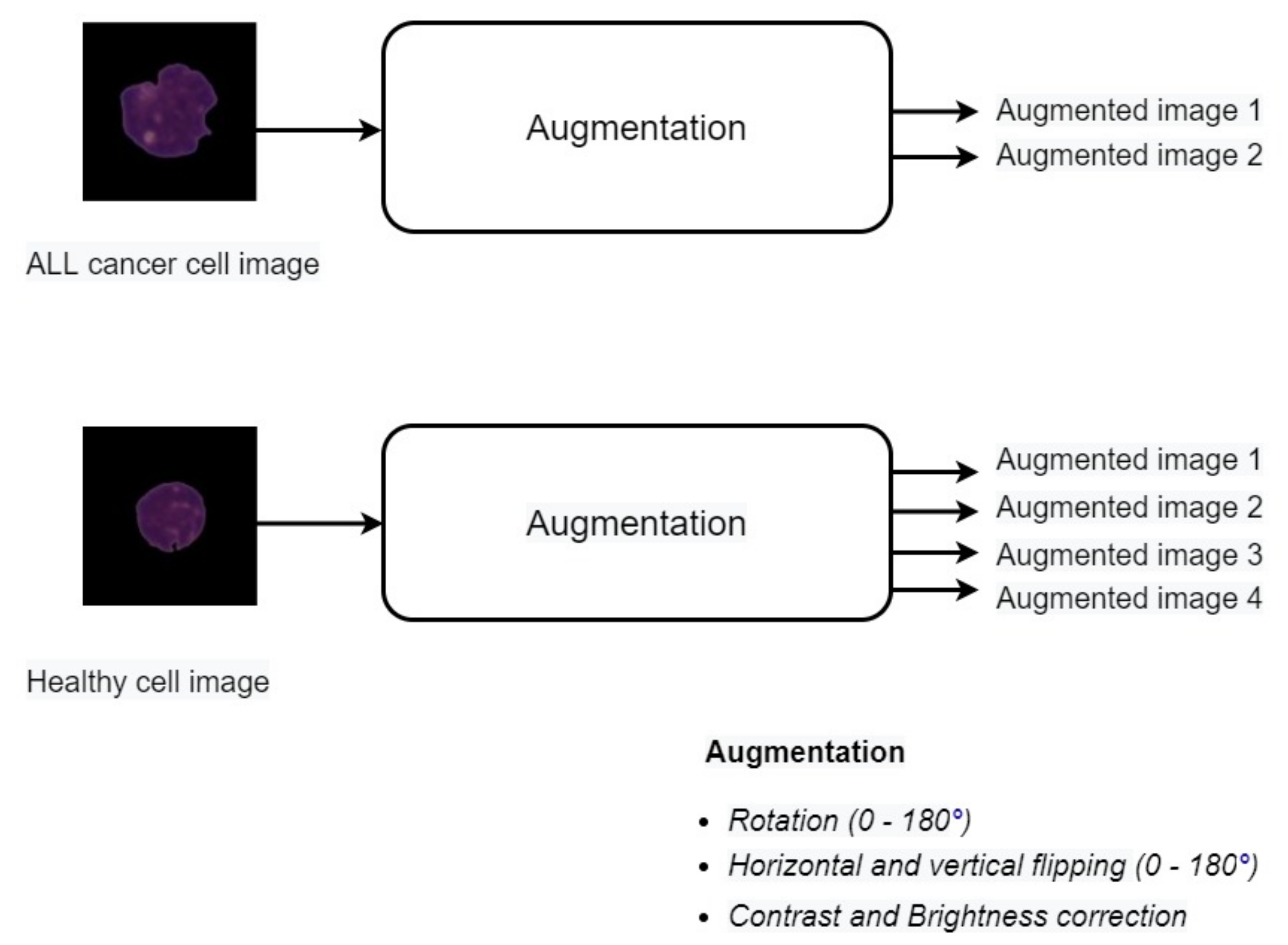
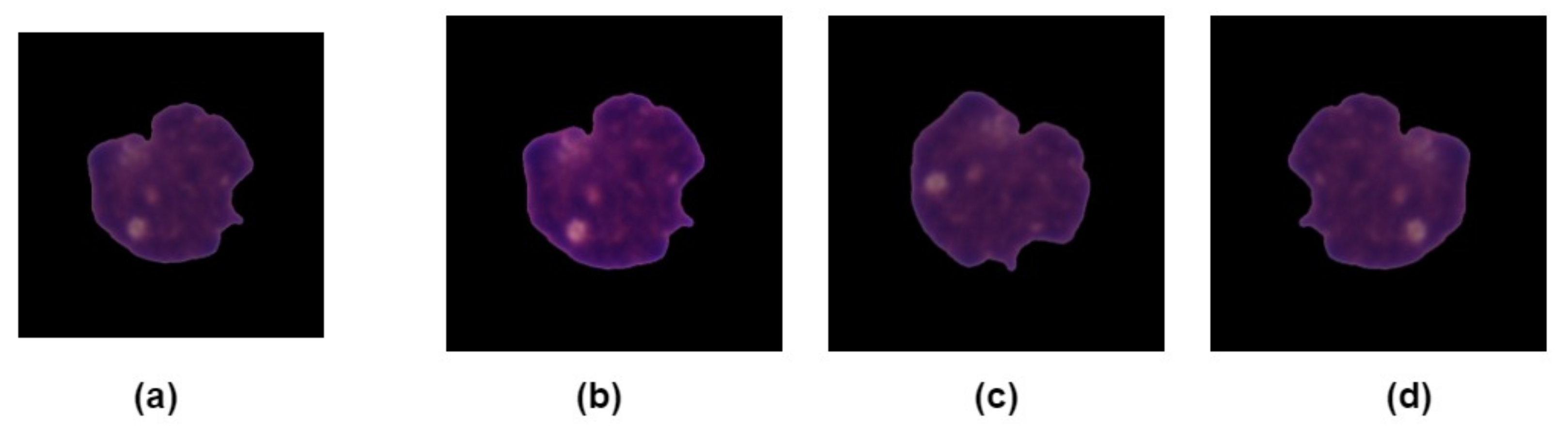
3.3. Data Augmentation

Data augmentation techniques can be used to overcome the problem of the limited size of a dataset, specifically in deep learning problems. Several techniques for image augmentation such as flipping, cropping, and rotation are used to obtain different copies of the original image. It gives the algorithm more generalization capabilities when we train our system not only with original images but with augmented images too. It has been stated that training a system with augmented images reduces the error rate and provides better generalization [41,42,43,44,45,46]. The CNM-C 2019 is an imbalanced dataset that may degrade the performance of deep learning models. Data imbalanced problems usually cause overfitting and lead the model towards poor generalization. In order to avoid the problem of overfitting and to increase the number of images in the dataset, we used different data augmentation techniques such as rotation, horizontal and vertical flip, brightness correction, and contrast adjustments on the training dataset. The augmentation on images is applied on the run for every single image. Every time the model gets an image, it loops through the image and generates four augmented images in case of healthy cell images and generates two images in case of ALL cancer cell images, as shown in Figure 2.

Random rotation is applied to rotate the images clockwise, according to the value between (−45 to 45) degrees. Horizontal and vertical flipping was also applied on images to horizontally and vertically flip the entire rows and columns of an image to produce a mirror image.

Table 2. Dataset distribution before and after data augmentation for each fold.

		Cancer Cell Images
Fold	Before Augmentation	After Augmentation
1	1119	2238
2	1100	2200
3	1200	2400
4	1248	2436
5	1203	2406
6	1209	2418
Total	7049	14,098
		Normal Cell Images
Fold	Before Augmentation	After Augmentation
1	562	2248
2	473	1892
3	538	2152
4	541	2164
5	524	2096
6	538	2152
Total	3176	12,704

represents our dataset distribution before and after augmentation for each fold, while Figure 3 represents the images before and after augmentation. There is a smaller number of healthy cell images than ALL cancer cell images in the C-NMC dataset. Therefore, to balance the dataset class-wise, we randomly applied the mentioned augmentation techniques on every image. These augmentation techniques always vary between flipping, rotation, contrast, and brightness correction. The healthy images are augmented at a double rate than ALL cancer cells to produce an equal number of images of both classes. Whenever the model gets an image, it generates two augmented images in the case of cancer cell images and four augmented images in the case of normal cell images.

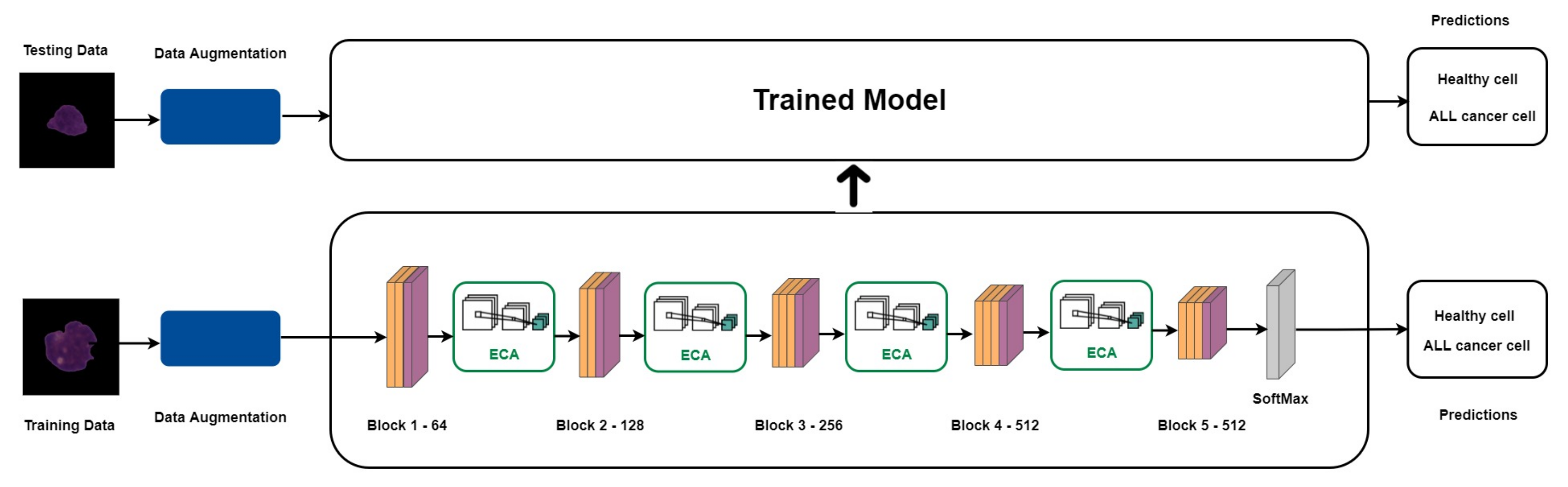
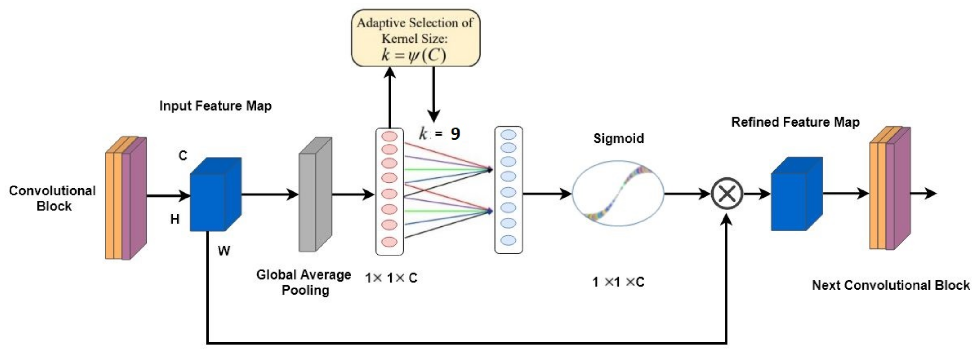
3.4. ECA-Net Based on VGG16

The Overall Architecture

The proposed model is based on VGG16, which is one of the famous CNN architecture that won the ImageNet large-scale visual recognition challenge (ILSVR) competition in 2014. There are two big motivations behind using VGG16 as our backbone model for ALL classification.

Table 3. The plain VGG16 model parameters in detail [51].

Layer Name	Input Shape	Output Shape	Stride	Conv Kernel Size
Conv1-1-64	224 × 224 × 3	224 × 224 × 64	1	3 × 3
Conv1-1-64	224 × 224 × 64	224 × 224 × 64	1	3 × 3
Maxpool-1	224 × 224 × 64	112 × 112 × 64	2	2 × 2
Conv2-1-128	112 × 112 × 64	112 × 112 × 128	1	3 × 3
Conv2-1-128	112 × 112 × 128	112 × 112 × 128	1	3 × 3
Maxpool-2	112 × 112 × 128	56 × 56 × 128	2	2 × 2
Conv3-1-256	56 × 56 × 128	56 × 56 × 256	1	3 × 3
Conv3-1-256	56 × 56 × 256	56 × 56 × 256	1	3 × 3
Maxpool-3	56 × 56 × 256	28 × 28 × 256	2	2 × 2
Conv4-1-512	28 × 28 × 256	28 × 28 × 512	1	3 × 3
Conv4-1-512	28 × 28 × 512	28 × 28 × 512	1	3 × 3
Maxpool-4	28 × 28 × 512	14 × 14 × 512	2	2 × 2
Conv5-1-512	14 × 14 × 512	14 × 14 × 512	1	3 × 3
Conv5-1-512	14 × 14 × 512	14 × 14 × 512	1	3 × 3
Maxpool-4	14 × 14 × 512	7 × 7 × 512	2	2 × 2
Fully connected-1	1 × 1 × 25,088	1 × 1 × 4096	1	1 × 1
Fully connected-2	1 × 1 × 4096	1 × 1 × 4096	1	1 × 1
Fully connected-3	1 × 1 × 4096	1 × 1 × 1000	1	1 × 1

provides a comprehensive overview of plain VGG16. To begin with, it extracts the features at a low level by utilizing a smaller kernel size and fewer layers as compared to its counterpart VGG19 network and other deep learning models. Instead of having a huge number of hyper-parameters, the network follows a simple design, where each block of VGG16 consists of convolutional layers with 3 × 3 filters and unit stride. Max pooling layers of 2 × 2 windows with the stride of 2 is used to reduce the size of the image to half. Throughout the network, each block follows the same combinations of max pooling and convolution layers. In the end, it uses 3 fully connected layers (FC) for the output. The stacking of convolutional layers enables the network to capture more information with lesser computational overhead hierarchically. The newer deep learning models such as DenseNet [47], ResNet [48], Inception [49], etc. use a lot of convolution layers, whereas our objective was to create a simple deep learning model for ALL classification. Secondly, the VGG16 model has a higher feature extraction ability for the classification of ALL cell images as shown in [50]. The shallow network keeps more information about the underlying features, which is important for cell texture identification. The overall architecture of proposed model is shown in Figure 4.

To explore high value featured related to ALL in the input image, we use an attention module to force the network to learn the high-level features. Attention not only illustrates where it should be focused, but also enhances the representation of features. Wang et al. [52] proposed a local cross-channel interaction strategy which is realized via 1D convolution called ECA, which can be widely used to boost the representation power of CNNs. In addition, considering the complexity of ALL features, it is difficult for the traditional CNNs to train these images. VGG16 with an attention module is more suitable for the proposed problem due to the improvement of feature representation. The shallow convolution modules can only extract the edge and texture features. The deep convolution modules can provide more abstract semantic features, which can better distinguish between ALL cancer and healthy cell images. The ECA module is added to enhance and amplify the difference of semantic features extracted by VGG16. This model is expected to overcome the morphological similarity and further improve the classification performance. Moreover, the ECA module also allows the model to focus on more important channel features. The salient feature information is used by ECA attention to accomplish task adaptive feature pooling operation. The ECA module aids in medical image analysis to automatically learn to focus on target structures of various shapes and sizes. Intuitively, a model trained using the ECA module learns to suppress irrelevant regions in input images while emphasizing silent features for a given task to improve the accuracy and efficiency of a deep learning model. The architecture of the ECA module is shown in Figure 5.

Human biological processes are the best approaches to demonstrate the intuition behind attention. For example, in order to assist perception, our visual processing system selectively focuses on specific portions of the image regardless of extraneous information [53]. The ECA module extracts the information from each channel of VGG16 results in a weighted sum of all the aggregated features. This allows the deep learning model to assign greater weight to certain elements of the input images. In Section 4.2 we show the feature maps generated by our proposed method clearly presented that our model focused on the cell itself rather than the image background. Attention modules are used to help CNN learn and to focus on more important features, instead of learning non-useful context knowledge. In order to learn more deep features, ECA has been employed after every VGG16 block. The ECA module helps to avoid feature dimensionality reduction caused by the convolutional block which inevitably brings side effects and is conducive to capturing the dependency between the channels. The ECA module only involves few parameters to explores the local cross-channel interaction by implementing a 1 × 1 convolution via adaptive selection of the kernel size k. In our proposed model we used k = 9 extra parameters with our backbone VGG16 following the original ECA paper. Gradient descent is also utilized to optimize these parameters. ECA module can increase the information interaction between channels of the feature maps, reduce the model complexity, and maintains the performance.

After the global average pooling (GAP), the ECA module considers each channel of the input feature maps and its k nearest neighbors, and quickly completes the channel weight calculation through one-dimensional convolution. Where k represents the number of neighboring channels involved in the calculation of a channel weight, and the value of k affects the efficiency and effectiveness of the ECA. The ECA module helps to adaptively compute k via a function of channel dimension C, and then performs 1D convolution followed by a sigmoid function to learn channel attention.

3.5. Experimental Setting

In our experiments, we resized the cell images to 224 × 224 resolution. The learning rate was set to 0.0001 with stochastic gradient descent (SGD) optimization and the network is trained for 50 epochs. The batch size is set as 16 in the training process. The cross entropy loss function is used as a loss function to train our model. The software environment used is Ubuntu 16.04, Python 3.5, and Pytorch 3.7. The hardware environment is CPU E5-2630 and a NVIDIA GV100GL Tesla V100 32GB graphics processing unit (GPU).

3.6. Evaluation Metrics

Five metrics, namely accuracy, sensitivity, precision, specificity, and F1 score are used to determine to evaluate the performance of the proposed method. Accuracy calculates the number of images correctly classified, divided by the total number of images in the test set, which is defined as:

$$\begin{array}{cc}\hfill Accuracy(\%)& =\frac{TP+TN}{TP+TN+FP+FN}\times 100\hfill \end{array}$$

(1)

Sensitivity (recall) or true positive rate (TPR) in the diagnosis of disease indicates the proportion of true positive outcomes over all actual positive cases (malignant cell images).

$$\begin{array}{cc}\hfill Sensitivity\left(Recall\right)(\%)& =\frac{TP}{TP+FN}\times 100\hfill \end{array}$$

(2)

Specificity or true negative rate (TNR) computes the true proportion of all true negative outcomes (normal cell images).

$$\begin{array}{cc}\hfill Specificity(\%)& =\frac{TN}{TN+FP}\times 100\hfill \end{array}$$

(3)

The precision is measured as the actual number of accurately labeled positive samples over the total number of positive samples (either correctly or incorrectly). The precision measures the model’s accuracy in classifying a sample as positive.

$$\begin{array}{cc}\hfill Precision(\%)& =\frac{TP}{TP+FP}\times 100\hfill \end{array}$$

(4)

F1 score is measured as the weighted average of sensitivity and precision. Therefore, this score takes both false positives and false negatives into account.

$$\begin{array}{cc}\hfill F1-score(\%)& =2\times \frac{(precision\times recall)}{(precision+recall)}\times 100\hfill \end{array}$$

(5)

4. Results

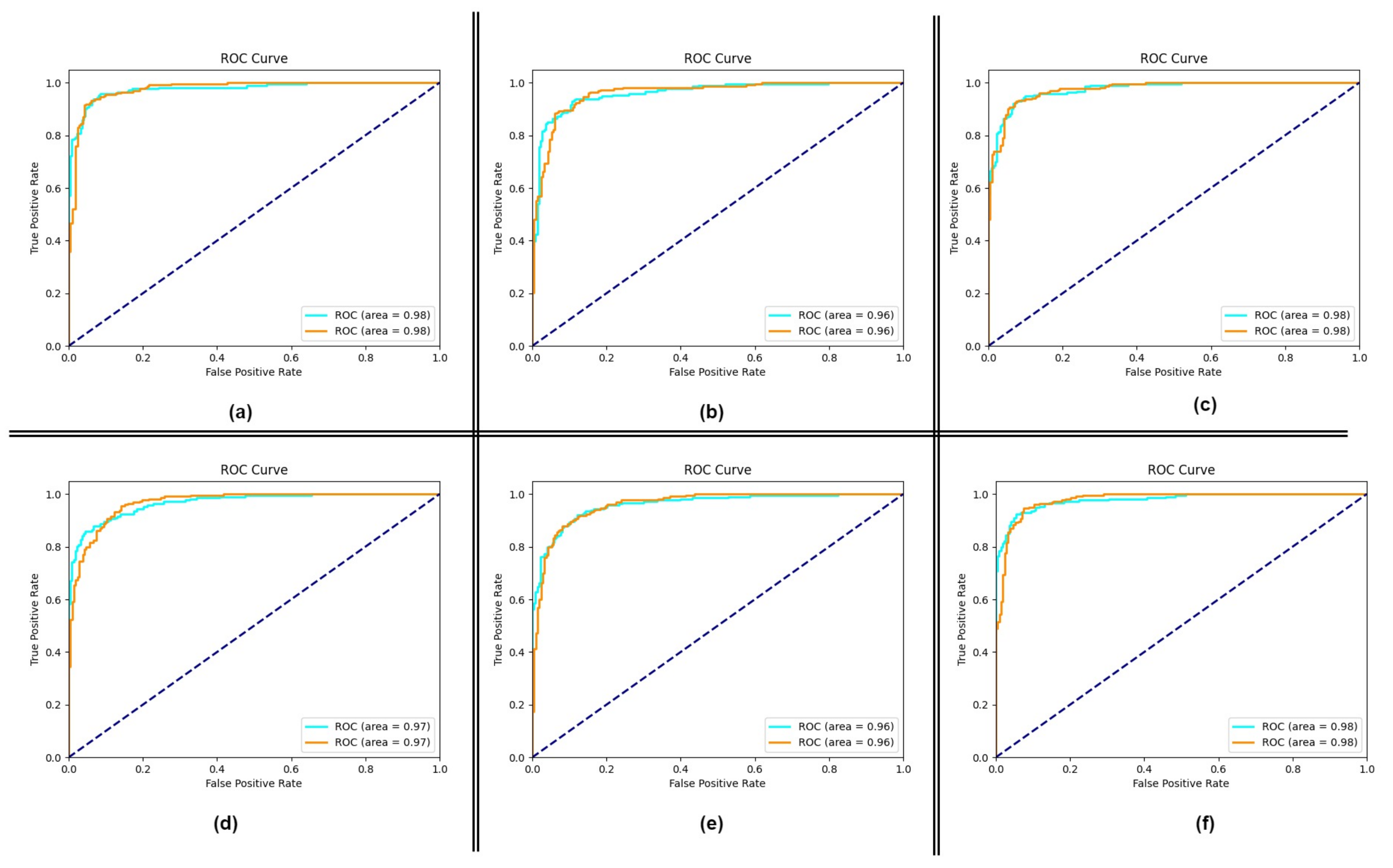
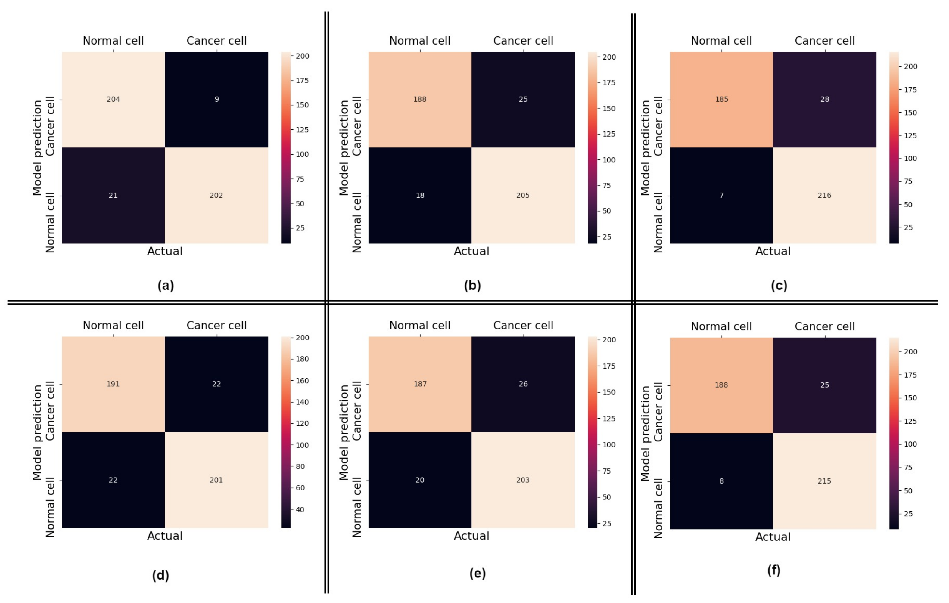
4.1. Performance of the Proposed Method

The original dataset is three-fold. We used the three-fold dataset and split it into seven folds based on subject-level variability. As a result, the experiment is performed six times with various combinations of training data each time. We first train/validate our model using fold-1 data and test it using fold-7 data for final accuracy. We apply the same strategy to the other remaining five folds. Fold-7 is only used to test the efficiency of our proposed model. The dataset is divided based on subject-level instead of image level. Furthermore, we divided the training set into 20% for model validation. The validation dataset is usually used to tune the hyperparameters such as the learning rate, number of epochs, etc. In our experiment, we set the epochs to 50. Our model is simple, which typically reaches an optimal point on the epochs between 40 to 45, and then possibly it stops converging. We used a validation set to get the best model while training. For example, whenever the model achieves good accuracy on the validation set in the training phase, it saves the best model with the best parameters. Later, we test this model using testing data to come up with overall accuracy. In order to verify the robustness of the model, we use different folds to train the model and calculate the average accuracy and standard deviation for each fold. Finally, the six performance estimates are summed to get an overall assessment of the classifier.

Table 4. Accuracy and standard deviation of our proposed model and plain VGG16 over 6-fold cross-validation. Each column in the table represents the fold number. The bold value represents the best performance among 6 folds, while the underline value shows the second best performance.

Methods	Fold-1	Fold-2	Fold-3	Fold-4	Fold-5	Fold-6	Mean	Std
VGG16 + Attention	0.931	0.901	0.919	0.899	0.894	0.924	0.911	0.013
VGG16	0.862	0.837	0.841	0.823	0.818	0.855	0.839	0.015

present the results of each fold’s performance for VGG16 with and without attention module. Our proposed VGG16 with the ECA module outperforms plain VGG16 by identifying the most pertinent information in an input image and aids in classification accuracy. Adding the ECA module helps the model increase the model performance (the attention module does not ignore the irrelevant features, but it just diminishes their importance).

Table 5. The evaluation metrics of the proposed model (VGG16 with attention) for ALL classification.

Folds	Accuracy	Sensitivity (Recall)	Specificity	Precision	F1 Score
Fold-1	0.931	0.906	0.957	0.957	0.930
Fold-2	0.901	0.912	0.891	0.882	0.891
Fold-3	0.919	0.963	0.885	0.868	0.913
Fold-4	0.899	0.896	0.901	0.901	0.898
Fold-5	0.894	0.903	0.886	0.877	0.889
Fold-6	0.924	0.959	0.895	0.882	0.918

and

Table 6. The evaluation metrics for plain VGG16.

Folds	Accuracy	Sensitivity (Recall)	Specificity	Precision	F1 Score
Fold-1	0.862	0.873	0.852	0.840	0.856
Fold-2	0.837	0.831	0.842	0.825	0.832
Fold-3	0.841	0.839	0.843	0.835	0.836
Fold-4	0.823	0.820	0.825	0.816	0.817
Fold-5	0.818	0.813	0.824	0.816	0.814
Fold-6	0.855	0.871	0.841	0.826	0.847

represent the evaluation matrices of VGG16 with and without attention module obtained from different folds. In ALL classification, we can see that fold-1 produces the best mean accuracy result for cancer and healthy cell images. We can presume that the sample selection for the training set can significantly affect the performance results. Figure 6 provided the receiver operating characteristic (ROC) curves generated in different folds on testing data, while Figure 7 shows the confusion matrices obtained from the proposed method. It can be seen that the proposed method successfully identified most of the cell images in their respective classes. The obtained results suggested that the ECA module helps to improve the model prediction. We tested our approach using six-fold cross-validation since it produces more trustworthy findings in evaluation.

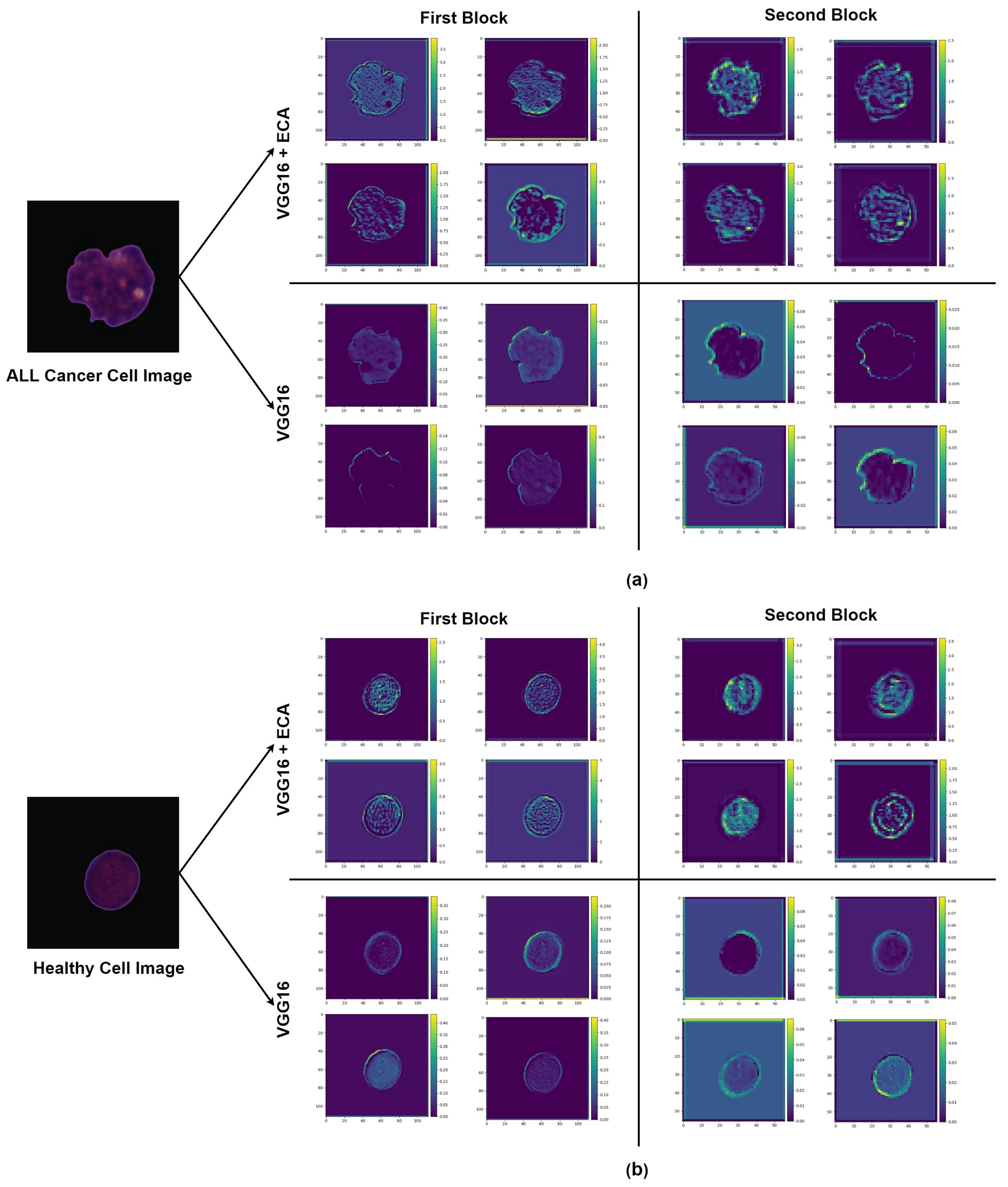
4.2. Impact of Using Attention

To test the efficiency of the attention module, we show the feature maps of the first and second block of VGG16 with and without attention module for the classification of ALL cancer and healthy cell images. We used plain VGG16 and VGG16 with attention to classify ALL cell images. Figure 8 illustrates the feature maps of ALL cancer and healthy cell images generated by the first and second blocks of VGG16 with and without the ECA module. The results indicated that the ECA module can enable the VGG16 model to automatically highlight the relevant features of the input images which, in ALL, is typically the whole cell area with the edges to improve the model performance. The feature maps generated with the ECA module spotlight more on the cell area and edges as compared to plain VGG16.

4.3. Comparisons with Other Approaches

Comparison of our proposed method with existing methods is provided in

Table 7. Performance comparisons between our proposed method and other approaches.

Methods	Accuracy	Year
NASNet-Large with VGG19 [36]	0.965	2020
Hybrid model (VGG16 + MobileNet) [37]	0.961	2019
LeukoNet [38]	0.896	2018
Proposed Method	0.911	2021

. These methods used the training part of the C-NMC 2019 dataset, but they did not consider the subject-level variability. They took the initial training (three-fold) part of the dataset and split the data into testing, training, and validation sets. However, it should be noted that no cross-validation was used in the evaluation, and how the test and training sets were chosen is unknown. In our proposed method, we split the training data of the C-NMC 2019 challenge into seven folds by keeping the subject-level variability in mind, which was ignored by previously proposed methods. We split the dataset so that all of the cell images belonging to the same subject are placed in the same fold, and not a single fold includes cell images from the same subject. It is observed that our proposed method gives satisfactory results as compared to the methods proposed in the literature. Classifying ALL cell images is challenging because of the morphological similarities between ALL cancer and healthy cell images and subject-level variability.

Table 8. Methods with the top entry of C-NMC 2019 Challenge.

Methods	F1-Score
SDCT-AuxNet [35]	0.948
Neighborhood-correction algorithm (NCA) [54]	0.910
Ensemble model based on MobileNetV2 [55]	0.894
Deep Multi-model Ensemble Network (DeepMEN) [50]	0.885
Ensemble CNN based on SENet and PNASNet [56]	0.879
Deep Bagging Ensemble Learning [57]	0.876
LSTM-DENSE [58]	0.866
Ensemble CNN model [59]	0.855
Multi-stream model [60]	0.848

presented methods with the top entry of the C-NMC 2019 Challenge. These methods used the C-NMC 2019 dataset’s three sets, i.e., training set, preliminary test composition, and final test set composition. They have only reported the F-1 score of their model performance and did not provide the results concerning other evaluation metrics for the classification of ALL.

5. Discussion

In this paper, a CNN-based method for the classification of ALL cancer and healthy cell images has been proposed. The proposed model is an enhancement of VGG16 CNN architecture. The attention module not only shows where attention should be taken, but it also improves feature representation. The results show that our proposed method based on the ECA module is able to extract and fuse deep features with a mean test accuracy of 0.911 in ALL classification.

By referring to the classification results, it is obvious that although our proposed method is relatively simple, it obtains acceptable performance for the ALL diagnosis. Hence, the proposed algorithm can be used as an assisting diagnostic tool for pathologists. Furthermore, the clinical impact of this research is that it helps the pathologists to examine a blood smear for finding cancerous cells. It should be noted that, from the performance comparisons of different networks, certain networks performed poorly which is not surprising considering the morphological similarity between the normal and cancerous cells. To conclude, the attention module can increase the CNN model’s efficiency in ALL classification. The proposed attention-based CNN has better adaptability, robustness, and classification accuracy than the state-of-art deep learning-based approaches. In this work, we have used only C-NMC 2019 training set for binary classification. As a future work direction, the model could easily be extended for multi-class classification and can be evaluated different data datasets of same or similar disease.

6. Conclusions

In this study, we proposed a diagnostic support system based on CNN architecture with an ECA module to accurately classify ALL cancer and healthy cell images. VGG16 is used as our backbone to extract the features from the source images. The ECA module was incorporated after each convolutional block to further enhance the relevance of extracted features from VGG16. The performance comparison between the VGG16 model with and without the ECA module showed that the attention mechanism helps in improving the model accuracy since it explores the relationship between channels and obtains better feature representation. The findings of this study revealed that our proposed deep learning-based model outperforms the state-of-the-art approaches. Integrating the attention module in the deep learning architectures may yield a significant performance gain. We evaluated our method on the C-NMC 2019 dataset. The obtained results showed a mean accuracy of 0.911 on this challenging dataset. In the future researchers can focus more on reducing the false positive rate to further improve the final accuracy.

References

1. Laosai, J.; Chamnongthai, K. Classification of acute leukemia using medical-knowledge-based morphology and CD marker. Biomed. Signal Process. Control 2018, 44, 127–137. [Google Scholar] [CrossRef]
2. Vogado, L.H.; Veras, R.M.; Araujo, F.H.; Silva, R.R.; Aires, K.R. Leukemia diagnosis in blood slides using transfer learning in CNNs and SVM for classification. Eng. Appl. Artif. Intell. 2018, 72, 415–422. [Google Scholar] [CrossRef]
3. American Society of Hematology. Hematology. Available online: https://www.hematology.org (accessed on 24 April 2021).
4. Key Statistics for Acute Lymphocytic Leukemia. American Cancer Society. Available online: https://www.cancer.org/cancer/acute-lymphocytic-leukemia/about/key-statistics.html (accessed on 24 April 2021).
5. Curesearch for Childrens Cancer Research. Curesearch. Available online: https://curesearch.org/Acute-Lymphoblastic-Leukemia-in-Children (accessed on 20 April 2021).
6. Mohamed, M.; Far, B.; Guaily, A. An efficient technique for white blood cells nuclei automatic segmentation. In Proceedings of the 2012 IEEE International Conference on Systems, Man, and Cybernetics (SMC), Seoul, Korea, 14–17 October 2012; pp. 220–225. [Google Scholar]
7. Amin, M.M.; Kermani, S.; Talebi, A.; Oghli, M.G. Recognition of acute lymphoblastic leukemia cells in microscopic images using k-means clustering and support vector machine classifier. J. Med. Signals Sens. 2015, 5, 49. [Google Scholar]
8. Duggal, R.; Gupta, A.; Gupta, R. Segmentation of overlapping/touching white blood cell nuclei using artificial neural networks. CME Series on Hemato-Oncopathology; All India Institute of Medical Sciences (AIIMS): New Delhi, India, 2016. [Google Scholar]
9. Duggal, R.; Gupta, A.; Gupta, R.; Mallick, P. SD-layer: Stain deconvolutional layer for CNNs in medical microscopic imaging. In Proceedings of the International Conference on Medical Image Computing and Computer-Assisted Intervention, Quebec City, QC, Canada, 10–14 September 2017; pp. 435–443. [Google Scholar]
10. Duggal, R.; Gupta, A.; Gupta, R.; Wadhwa, M.; Ahuja, C. Overlapping cell nuclei segmentation in microscopic images using deep belief networks. In Proceedings of the Tenth Indian Conference on Computer Vision, Graphics and Image Processing, Guwahati, India, 18–22 December 2016; pp. 1–8. [Google Scholar]
11. Gupta, A.; Duggal, R.; Gehlot, S.; Gupta, R.; Mangal, A.; Kumar, L.; Thakkar, N.; Satpathy, D. GCTI-SN: Geometry-inspired chemical and tissue invariant stain normalization of microscopic medical images. Med. Image Anal. 2020, 65, 101788. [Google Scholar] [CrossRef]
12. Gupta, R.; Mallick, P.; Duggal, R.; Gupta, A.; Sharma, O. Stain color normalization and segmentation of plasma cells in microscopic images as a prelude to development of computer assisted automated disease diagnostic tool in multiple myeloma. Clin. Lymphoma Myeloma Leuk. 2017, 17, e99. [Google Scholar] [CrossRef]
13. Bayramoglu, N.; Heikkilä, J. Transfer learning for cell nuclei classification in histopathology images. In Proceedings of the European Conference on Computer Vision, Amsterdam, The Netherlands, 11–14 October 2016; pp. 532–539. [Google Scholar]
14. Gao, Z.; Wang, L.; Zhou, L.; Zhang, J. HEp-2 cell image classification with deep convolutional neural networks. IEEE J. Biomed. Health Inform. 2016, 21, 416–428. [Google Scholar] [CrossRef] [Green Version]
15. Zhao, J.; Zhang, M.; Zhou, Z.; Chu, J.; Cao, F. Automatic detection and classification of leukocytes using convolutional neural networks. Med. Biol. Eng. Comput. 2017, 55, 1287–1301. [Google Scholar] [CrossRef]
16. Joshi, M.D.; Karode, A.H.; Suralkar, S. White blood cells segmentation and classification to detect acute leukemia. Int. J. Emerg. Trends Technol. Comput. Sci. (IJETTCS) 2013, 2, 147–151. [Google Scholar]
17. Mohapatra, S.; Patra, D.; Satpathy, S. An ensemble classifier system for early diagnosis of acute lymphoblastic leukemia in blood microscopic images. Neural Comput. Appl. 2014, 24, 1887–1904. [Google Scholar] [CrossRef]
18. Putzu, L.; Caocci, G.; Di Ruberto, C. Leucocyte classification for leukaemia detection using image processing techniques. Artif. Intell. Med. 2014, 62, 179–191. [Google Scholar] [CrossRef] [Green Version]
19. Singhal, V.; Singh, P. Local binary pattern for automatic detection of acute lymphoblastic leukemia. In Proceedings of the 2014 Twentieth National Conference on Communications (NCC), Kanpur, India, 28 February–2 March 2014; pp. 1–5. [Google Scholar]
20. Patel, N.; Mishra, A. Automated leukaemia detection using microscopic images. Procedia Comput. Sci. 2015, 58, 635–642. [Google Scholar] [CrossRef] [Green Version]
21. Karthikeyan, T.; Poornima, N. Microscopic image segmentation using fuzzy c means for leukemia diagnosis. Int. J. Adv. Res. Sci. Eng. Technol. 2017, 4, 3136–3142. [Google Scholar]
22. Mohamed, H.; Omar, R.; Saeed, N.; Essam, A.; Ayman, N.; Mohiy, T.; AbdelRaouf, A. Automated detection of white blood cells cancer diseases. In Proceedings of the 2018 First International Workshop on Deep and Representation Learning (IWDRL), Cairo, Egypt, 29 March 2018; pp. 48–54. [Google Scholar]
23. Rajpurkar, P.; Irvin, J.; Zhu, K.; Yang, B.; Mehta, H.; Duan, T.; Ding, D.; Bagul, A.; Langlotz, C.; Shpanskaya, K.; et al. Chexnet: Radiologist-level pneumonia detection on chest x-rays with deep learning. arXiv 2017, arXiv:1711.05225. [Google Scholar]
24. Yan, Z.; Zhan, Y.; Peng, Z.; Liao, S.; Shinagawa, Y.; Metaxas, D.N.; Zhou, X.S. Bodypart recognition using multi-stage deep learning. In Proceedings of the International Conference on Information Processing in Medical Imaging, Sabhal Mor Ostaig/Isle of Skye, UK, 28 June–3 July 2015; pp. 449–461. [Google Scholar]
25. Sermanet, P.; Eigen, D.; Zhang, X.; Mathieu, M.; Fergus, R.; LeCun, Y. Overfeat: Integrated recognition, localization and detection using convolutional networks. arXiv 2013, arXiv:1312.6229. [Google Scholar]
26. Yang, X.; Kwitt, R.; Styner, M.; Niethammer, M. Quicksilver: Fast predictive image registration–a deep learning approach. NeuroImage 2017, 158, 378–396. [Google Scholar] [CrossRef] [PubMed]
27. Stefano, A.; Comelli, A. Customized Efficient Neural Network for COVID-19 Infected Region Identification in CT Images. J. Imaging 2021, 7, 131. [Google Scholar] [CrossRef]
28. Comelli, A.; Dahiya, N.; Stefano, A.; Vernuccio, F.; Portoghese, M.; Cutaia, G.; Bruno, A.; Salvaggio, G.; Yezzi, A. Deep learning-based methods for prostate segmentation in magnetic resonance imaging. Appl. Sci. 2021, 11, 782. [Google Scholar] [CrossRef] [PubMed]
29. Rehman, A.; Abbas, N.; Saba, T.; Rahman, S.I.u.; Mehmood, Z.; Kolivand, H. Classification of acute lymphoblastic leukemia using deep learning. Microsc. Res. Tech. 2018, 81, 1310–1317. [Google Scholar] [CrossRef]
30. Shafique, S.; Tehsin, S. Acute lymphoblastic leukemia detection and classification of its subtypes using pretrained deep convolutional neural networks. Technol. Cancer Res. Treat. 2018, 17, 1533033818802789. [Google Scholar] [CrossRef] [PubMed] [Green Version]
31. Habibzadeh, M.; Jannesari, M.; Rezaei, Z.; Baharvand, H.; Totonchi, M. Automatic white blood cell classification using pre-trained deep learning models: Resnet and inception. In Proceedings of the Tenth International Conference on Machine Vision (ICMV 2017), International Society for Optics and Photonics, Vienna, Austria, 13–15 November 2017; Volume 10696, p. 1069612. [Google Scholar]
32. Ahmed, N.; Yigit, A.; Isik, Z.; Alpkocak, A. Identification of leukemia subtypes from microscopic images using convolutional neural network. Diagnostics 2019, 9, 104. [Google Scholar] [CrossRef] [PubMed] [Green Version]
33. Wang, Q.; Wang, J.; Zhou, M.; Li, Q.; Wang, Y. Spectral-spatial feature-based neural network method for acute lymphoblastic leukemia cell identification via microscopic hyperspectral imaging technology. Biomed. Opt. Express 2017, 8, 3017–3028. [Google Scholar] [CrossRef] [Green Version]
34. Pansombut, T.; Wikaisuksakul, S.; Khongkraphan, K.; Phon-On, A. Convolutional neural networks for recognition of lymphoblast cell images. Comput. Intell. Neurosci. 2019, 2019. [Google Scholar] [CrossRef]
35. Gehlot, S.; Gupta, A.; Gupta, R. SDCT-AuxNetθ: DCT augmented stain deconvolutional CNN with auxiliary classifier for cancer diagnosis. Med. Image Anal. 2020, 61, 101661. [Google Scholar] [CrossRef] [PubMed]
36. Kasani, P.H.; Park, S.W.; Jang, J.W. An Aggregated-Based Deep Learning Method for Leukemic B-lymphoblast Classification. Diagnostics 2020, 10, 1064. [Google Scholar] [CrossRef] [PubMed]
37. Kassani, S.H.; Kassani, P.H.; Wesolowski, M.J.; Schneider, K.A.; Deters, R. A hybrid deep learning architecture for leukemic B-lymphoblast classification. In Proceedings of the 2019 International Conference on Information and Communication Technology Convergence (ICTC), Jeju Island, Korea, 16–18 October 2019; pp. 271–276. [Google Scholar]
38. Kant, S.; Kumar, P.; Gupta, A.; Gupta, R. Leukonet: Dct-based cnn architecture for the classification of normal versus leukemic blasts in b-all cancer. arXiv 2018, arXiv:1810.07961. [Google Scholar]
39. Labati, R.D.; Piuri, V.; Scotti, F. All-IDB: The acute lymphoblastic leukemia image database for image processing. In Proceedings of the 2011 18th IEEE International Conference on Image Processing, Brussels, Belgium, 11–14 September 2011; pp. 2045–2048. [Google Scholar]
40. Iqbal, S.; Ghani, M.U.; Saba, T.; Rehman, A. Brain tumor segmentation in multi-spectral MRI using convolutional neural networks (CNN). Microsc. Res. Tech. 2018, 81, 419–427. [Google Scholar] [CrossRef] [PubMed]
41. Cireşan, D.C.; Meier, U.; Masci, J.; Gambardella, L.M.; Schmidhuber, J. High-performance neural networks for visual object classification. arXiv 2011, arXiv:1102.0183. [Google Scholar]
42. Krizhevsky, A.; Sutskever, I.; Hinton, G.E. Imagenet classification with deep convolutional neural networks. Adv. Neural Inf. Process. Syst. 2012, 25, 1097–1105. [Google Scholar] [CrossRef]
43. Wong, S.C.; Gatt, A.; Stamatescu, V.; McDonnell, M.D. Understanding data augmentation for classification: When to warp? In Proceedings of the 2016 International Conference on Digital Image Computing: Techniques and Applications (DICTA), Gold Coast, Australia, 30 November–2 December 2016; pp. 1–6. [Google Scholar]
44. Perez, L.; Wang, J. The effectiveness of data augmentation in image classification using deep learning. arXiv 2017, arXiv:1712.04621. [Google Scholar]
45. Shijie, J.; Ping, W.; Peiyi, J.; Siping, H. Research on data augmentation for image classification based on convolution neural networks. In Proceedings of the 2017 Chinese Automation Congress (CAC), Jinan, China, 20–22 October 2017; pp. 4165–4170. [Google Scholar]
46. Mikołajczyk, A.; Grochowski, M. Data augmentation for improving deep learning in image classification problem. In Proceedings of the 2018 International Interdisciplinary PhD Workshop (IIPhDW), Swinoujscie, Poland, 9–12 May 2018; pp. 117–122. [Google Scholar]
47. Huang, G.; Liu, Z.; Van Der Maaten, L.; Weinberger, K.Q. Densely connected convolutional networks. In Proceedings of the IEEE Conference on Computer Vision and Pattern Recognition, Honolulu, HI, USA, 21–26 July 2017; pp. 4700–4708. [Google Scholar]
48. He, K.; Zhang, X.; Ren, S.; Sun, J. Deep residual learning for image recognition. In Proceedings of the IEEE Conference on Computer Vision and Pattern Recognition, Las Vegas, NV, USA, 26–27 June 2016; pp. 770–778. [Google Scholar]
49. Szegedy, C.; Liu, W.; Jia, Y.; Sermanet, P.; Reed, S.; Anguelov, D.; Erhan, D.; Vanhoucke, V.; Rabinovich, A. Going deeper with convolutions. In Proceedings of the IEEE Conference on Computer Vision and Pattern Recognition, Boston, MA, USA, 7–12 June 2015; pp. 1–9. [Google Scholar]
50. Xiao, F.; Kuang, R.; Ou, Z.; Xiong, B. DeepMEN: Multi-model Ensemble Network for B-Lymphoblast Cell Classification. In Proceedings of the ISBI 2019 C-NMC Challenge: Classification in Cancer Cell Imaging, Venicee, Italy, 8–11 April 2019; pp. 83–93. [Google Scholar]
51. Simonyan, K.; Zisserman, A. Very deep convolutional networks for large-scale image recognition. arXiv 2014, arXiv:1409.1556. [Google Scholar]
52. Qilong, W.; Banggu, W.; Pengfei, Z.; Peihua, L.; Wangmeng, Z.; Qinghua, H. ECA-Net: Efficient Channel Attention for Deep Convolutional Neural Networks. In Proceedings of the IEEE Conference on Computer Vision and Pattern Recognition, (CVPR), Seattle, WA, USA, 16–18 June 2020. [Google Scholar]
53. Xu, K.; Ba, J.; Kiros, R.; Cho, K.; Courville, A.; Salakhudinov, R.; Zemel, R.; Bengio, Y. Show, attend and tell: Neural image caption generation with visual attention. In Proceedings of the International Conference on Machine Learning, PMLR, Lille, France, 7–9 July 2015; pp. 2048–2057. [Google Scholar]
54. Pan, Y.; Liu, M.; Xia, Y.; Shen, D. Neighborhood-correction algorithm for classification of normal and malignant cells. In Proceedings of the ISBI 2019 C-NMC Challenge: Classification in Cancer Cell Imaging, Venicee, Italy, 8–11 April 2019; pp. 73–82. [Google Scholar]
55. Verma, E.; Singh, V. ISBI Challenge 2019: Convolution Neural Networks for B-ALL Cell Classification. In Proceedings of the ISBI 2019 C-NMC Challenge: Classification in Cancer Cell Imaging, Venicee, Italy, 8–11 April 2019; pp. 131–139. [Google Scholar]
56. Shi, T.; Wu, L.; Zhong, C.; Wang, R.; Zheng, W. Ensemble Convolutional Neural Networks for Cell Classification in Microscopic Images. In Proceedings of the ISBI 2019 C-NMC Challenge: Classification in Cancer Cell Imaging, Venicee, Italy, 8–11 April 2019; pp. 43–51. [Google Scholar]
57. Liu, Y.; Long, F. Acute lymphoblastic leukemia cells image analysis with deep bagging ensemble learning. In Proceedings of the ISBI 2019 C-NMC Challenge: Classification in Cancer Cell Imaging, Venicee, Italy, 8–11 April 2019; pp. 113–121. [Google Scholar]
58. Shah, S.; Nawaz, W.; Jalil, B.; Khan, H.A. Classification of normal and leukemic blast cells in B-ALL cancer using a combination of convolutional and recurrent neural networks. In Proceedings of the ISBI 2019 C-NMC Challenge: Classification in Cancer Cell Imaging, Venicee, Italy, 8–11 April 2019; pp. 23–31. [Google Scholar]
59. Ding, Y.; Yang, Y.; Cui, Y. Deep learning for classifying of white blood cancer. In Proceedings of the ISBI 2019 C-NMC Challenge: Classification in Cancer Cell Imaging, Venicee, Italy, 8–11 April 2019; pp. 33–41. [Google Scholar]
60. Xie, X.; Li, Y.; Zhang, M.; Wu, Y.; Shen, L. Multi-streams and Multi-features for Cell Classification. In Proceedings of the ISBI 2019 C-NMC Challenge: Classification in Cancer Cell Imaging, Venicee, Italy, 8–11 April 2019; pp. 95–102. [Google Scholar]
Figure 1. ALL cell image samples from C-NMC 2019 dataset [8,9,10,11,12]. Images (AC) show ALL cancer cell images while (DF) show healthy cell images.
Applsci 11 10662 g001
Figure 2. The illustration of the image augmentation process.
Applsci 11 10662 g002
Figure 3. The result of applying data augmentation (bd). (a) Original image (b) brightness correction and contrast adjustments, (c) rotation, and (d) vertical and horizontal flipping.
Applsci 11 10662 g003
Figure 4. Our proposed model for the classification of ALL cell images.
Applsci 11 10662 g004
Figure 5. The ECA module takes the feature map, which is the output of a convolutional block and is 3-dimensional in shape (W × H × C). W, H, and C represent the width, height, and number of the feature map channels. The GAP reduces the dimensionality of the input feature map into 1 × 1 × C. Then the ECA module explores the local cross-channel interaction by implementing a 1 × 1 convolution via an adaptive selection of the kernel size k. After passing through the sigmoid function, the output channel weights of dimension 1 × 1 × C are used to refine the input feature map via element-wise product. Finally, the refined feature map is used as the input of the next convolutional block.
Applsci 11 10662 g005
Figure 6. The result of ROC curves obtained from different folds in our proposed model (a) shows the roc curve obtained from fold-1, (b) fold-2 roc curve, (c) fold-3 roc curve, (d) fold-4 roc curve, (e) fold-5 roc curve, and (f) fold-6 roc curve for the classification of ALL cell images.
Applsci 11 10662 g006
Figure 7. The confusion matrices obtained from different folds in our proposed model. (a) shows the confusion matrix ordained from fold-1, (b) the fold-2 confusion matrix, (c) the fold-3 confusion matrix, (d) the fold-4 confusion matrix, (e) the fold-5 confusion matrix, and (f) the fold-6 confusion matrix for the classification of ALL cell images.
Applsci 11 10662 g007
Figure 8. Feature maps generated by the first and second block of VGG16 with and without the ECA module. (a) The feature maps of ALL cancer cell image (b) the feature maps of healthy cell image.
Applsci 11 10662 g008