1. Introduction
The accurate estimation of production possibility set (PPS) boundaries is crucial for performance analysis and efficient estimation. Different papers propose alternative approaches to handle the issue of estimating PPSs and their respective boundaries. Non-parametric data envelopment analysis (DEA) is possibly one of the most used linear programming (LP) approaches to build up piecewise PPS boundaries. DEA is a useful tool to evaluate decision making units (DMUs). Efficiency criterion can be considered as a number between 0 and 1 for evaluating a DMU in DEA. If the efficiency criterion for a DMU is 1, the mentioned DMU is efficient, else, it is inefficient. Evaluating DMUs in input-oriented, output-oriented, and combined-oriented radial and non-radial models were developed from a proposal by Farrell (1957) [
1], and were then followed by the development of the CCR model by Charnes et al. (1978) [
2]. The CCR model was then developed into the BCC model by Banker et al. (1984) [
3]. Additive models were then suggested to separate efficient and non-efficient DMUs [
4]. Tone (2001) proposed a slack based model which evaluates DMUs considering the relationship between CCR models [
5]. The Russel Graph Model (RGM) and the relationship between SBM and additive DEA models are very important subjects that have been studied [
6]. These models determine the benchmark for efficient DMUs, in addition to calculating efficiency and non-efficiency criterion of DMUs. Over three decades, extensive and useful studies on DEA have been undertaken to calculate DMU efficiencies [
7,
8] and to find DMU benchmarks [
9,
10]. Chen and Zhu (2020) completed efficient and non-efficient definitions on the basis of slack variables using the slack based method, and showed that additive slacks-based models (ASBM) and enhanced RGM are equal. Moreover, the authors showed that the simultaneous use of ASBM and network DEA models can create a comparable DEA score. Finding DMU targets in ASBM by eliminating convexity conditions can be investigated in practical studies [
11]. The use of non-radial FDH models based on ASBM can also be beneficial in practical studies.
Specifically, Free Disposal Hull (FDH) is a subclass of DEA models where DMUs are not projected on the piecewise convex envelope, but are projected on the actual maximal attainable boundary, which results in a staircase shape for the single input–output case. In other words, FDH, which was first introduced by Deprins et al. (1984), evaluates DMU efficiency by considering the closest inner approximation of the true non-convex (disposable) boundary [
12]. Many studies have been investigated FDH models. Soleimani-Damaneh et al. estimated returns-to-scale in FDH models [
13]. Soleimani-Damaneh and Rashidi proposed a polynomial-time algorithm to estimate returns to scale in FDH models [
14]. Mostafaee and Soleimani-Damaneh proposed the definition, characterization and calculation of global sub-increasing and global sub-decreasing returns to scale in FDH technologies [
15]. Fukuyama et al. measured efficiency with non-convex FDH technology [
16]. Manzari Tavakoli and Mostafaee studied FDH efficiency scores of units with network structures [
17]. Arfa et al. measured the efficiency of hospital cardiology wards using the FDH approach [
18]. Kerstens and Van De Woestyne reviewed solution methods for nonconvex FDH models and give some critical comments [
19]. Soleimani-Damaneh and Mostafaee identified the anchor points in FDH models [
20]. Mirmozaffari et al. proposed an improved DEA model based on SBM and FDH models [
21]. One issue that is frequently neglected in FDH models is the identification of DMU targets, which is a cumbersome task due to boundary non-convexity, especially when the number of inputs and outputs increase. A possible approach is to define a multiple objective function for measuring the closeness among the DMU under analysis and its eventual targets [
22].
Multiple objective linear programming (MOLP) is a form of multiple objective decision making (MODM). In MODM problems, more than one objective is considered in regard to the opinions of the decision maker (DM). Interactive methods (IMs) are a kind of MODM and MOLP methods. IMs explore the criterion space on the progressive definition of the DM’s preferences at each iteration [
23]. IMs have been used in some reported works [
24,
25]. Traditional DEA models tend to ignore the DM’s preferences and value judgment in the computation of the DMU targets, completely. The use of IMs allows the obtainment of DMU targets which have perfect adaptation for the DM’s preferences [
24]. An IM was applied for the extension of DEA to effectiveness analysis [
26]. The step method (STEM) that was introduced in 1971 [
27] is an IMs in MOLP, and has been reported in several studies [
28,
29,
30,
31]. To the best of our knowledge, STEM has not yet been used by researchers to find targets in non-radial FDH models which consider ASBM and enhanced Russel measures in variable return to scale technology (the first research gap).
Multiple criteria decision making (MCDM) is divided into multiple attribute decision making (MADM) and MODM. In situations where the data are fuzzy, a combination of DEA and fuzzy MCDM [
32,
33,
34] can be used for the development of the proposed technique. In this study, as the data of the second case study were deterministic, it was not necessary to use fuzzy methods.
FDH is a well-known subclass of DEA models and is based on two distinctive features that are reflected in the PPS boundary. First, FDH ensures that efficiency evaluations are affected only by actually observed performances. Secondly, FDH relies on the non-convexity assumption which satisfies free disposability in PPS. There is inherent computational complexity to solve FDH models. As a matter of fact, FDH models are mixed 0–1 LP, and solving them is difficult. In this regard, a ratio-based approach (RBA) is proposed to solve radial FDH models without solving any mathematical programming models [
13]. This approach has been employed by some other studies [
15,
20]. To the best of our knowledge, RBA is one of the most suitable suggested methods to find DMU targets of radial FDH models without solving any mathematical programming models. DMU target finding of non-radial FDH models without solving any mathematical programming models can be considered as another research gap. It can be achieved by extending RBA. As ASBM relates to enhanced Russel measures, finding non-radial DMU targets has been possible using extended RBA.
In Fars province pharmaceutical distributing companies (the second case study), there was a variable return to scale assumption. Moreover, as the combination of pharmaceutical distributing companies was impossible, using FDH models was beneficial. Non-radial FDH models based on ASBM in variable return to scale technology can therefore be considered in the proposal for a technique for finding DMU targets. Therefore, considering mentioned research gaps, two research questions have considered as follows:
- (1)
Is it possible to propose a technique to find all DMU targets in non-radial FDH models based on ASBM using IM?
- (2)
Is it possible to find DMU targets of non-radial FDH models in the proposed technique without solving any mathematical models?
A hybrid technique to answer the above two research questions with the following properties has been proposed as the innovation of this research:
- (a)
DMU target finding in non-radial FDH models based on ASBM are more realistic because they are based on a non-convexity assumption,
- (b)
Proposing a new LP formulation of ASBM,
- (c)
Applying IMs instead of regular DEA methods to find FDH models targets which have more adaptation to the DM’s preferences,
- (d)
Finding the required DMU targets in FDH models using an algorithm that works by checking some conditions for DMUs without solving of any mathematical models.
To the best of our knowledge, proposing a hybrid technique with the mentioned properties has not been reported until now. It is notable that, according to the practical view, the proposed technique will be beneficial if finding DMU targets in a studied organization is useful. According to the theoretical view, as the proposed technique works based on mathematical modelling, considering assumptions and determining suitable parameters to compose related models are important subjects, too. Therefore, to implement and generalize the results, practical and theoretical views should be simultaneously considered.
There are several outlier detection methods, such as parametric robust regression in statistics [
35] and non-parametric k-means in data mining [
36]. Moreover, a predictive DEA model for outlier detection was proposed, and a comprehensive set of simulation experiments were conducted to examine the relative performance of the suggested method with two popular mentioned methods under the influence of five factors. The results provide users with practical guidelines on how to choose appropriate methods to detect outliers [
37]. Outlier detection and investigation of the sensitivity of the modeling approach to outliers can be applied for the development of the proposed technique.
The paper is structured in following sections: first, the background on ASBM, MOLP, STEM, and RBA is provided. After that, a new hybrid technique is introduced to find DMU targets in non-radial FHD models based on ASBM. Finally, the presented technique is applied in two real case studies.
2. Background
In this section, ASBM, STEM to solve MOLP, and RBA for finding targets of radial FDH models are briefly described. The purpose of this section is to introduce the theoretical basis for finding targets of non-radial FDH models based on ASBM using STEM and extended RBA.
2.1. Additive Slack Based Model
Suppose
, j = 1, …, n by consuming m inputs
can produce s outputs
. The background of ASBM can be related to the additive model in Charnes et al. (1985) [
4] and Green et al. (1997) [
6]. Therefore, efficiency for output r of DMU
o is defined as
and non-efficiency for output r of DMU
o is defined as
. Furthermore, efficiency for input i of DMU
o is defined as
and non-efficiency for output r of DMU
o is defined as
. Therefore, by suggesting model (1), the relationship between non-efficiency calculated by Greek et al. (1997) [
6] and ASBM based on efficiency and non-efficiency definitions have presented [
11].
Model (1) is a nonlinear mathematical programming model containing linear constraints and linear fractional objective function. In this regard, model (1) by Chen and Zhu (2020) [
11] is equivalent to RGM developed by Fare et al. (1985). Moreover, finding DMU targets using slack variables are important because focus is given to the summation of slack variables. In this regard, the projection of DMU with respect to Model (1) is calculated by
and
which
and
are optimal solutions of Model (1).
2.2. MOLP and STEM
A general formulation of the MOLP problem is given in model 2.
where
represents the objective function vector. Linear objective functions are denoted by
where u = (u
1, …, u
v) is the decision-making vector. The symbol T is a transposed vector. g
l(u), C
l, and c
il are the l
th objective function, the vector of decision-making variable coefficients in the l
th objective function, and the coefficients of l
th objective function namely C
l, l = 1, …, k, per n existing variables, respectively. W is the feasible region of the MOLP problem and k is the number of the objective function. The decision-making variable multiples matrix is denoted by A, while b represents the right-hand side vector of the constraints.
is the constraints of the feasible region and
, representing the Euclidean space comprising all nonnegative vectors in a v-dimensional space. In this MOLP problem, the l
th objective function is formulated as
. The vector u* ∈ W is considered as an efficient (non-dominated) solution, if there does not exist another u ∈ W, such that g
l(u) ≥ g
l(u∗) for all l and g
l(u) > g
l(u∗) for at least one l.
STEM is an IM that can be used to solve MOLP problems. It works based on the obtained information from DM preferences and reduces the feasible region, step by step. STEM relies on DMs information to identify feasible and efficient solutions during the procedure. STEM includes following steps [
27,
30]:
- Step 0:
building-up the pay-off table
Objective functions should be optimized separately as follows (cf. model 3 and
Table 1):
The diagonal elements, represented by , are the optimal solutions for the single , l = 1, …, k problem obtained through the solving of model 3. zdl values are the results for dth objective function, computed upon the optimal solution obtained for lth objective function, l = 1, …, k, d = 1, …, k, .
- Step 1:
Calculation Phase
The computation of coefficients β
l, l = 1… k, is the cornerstone to compute the relative importance (Equation (4)) of each distance from the optimal objective function value. Suppose that π
l denotes the relative importance of the distance between objective functions and their optimal values. Although these coefficients are locally meaningful, they cannot capture the overall importance, unlike other utility models. It is therefore necessary to solve model 5, where the solution obtained in the p
th iteration is denoted by
.
and
. Model 5 is given as follows:
Wp represents the feasible region in the pth iteration. In order to find the vector u ∈ Wp, which provides the minimum of maximum distance between the objective function vector of and its optimal vector, , h should be minimized. h indicates the maximum distance of the functions from their optimal values based on their relative importance for each individual feasible solution in the feasible region. In other words, h indicates the closest possible distance to the optimal value of the lth objective function, that is . Before proceeding to Step 2, the minimum value in column l of the pay-off table should be picked up. It is denoted as .
- Step 2:
Decision Phase
In this phase, the DM provides relative importance information with respect to the solution collected during the first step of the p
th iteration, that is
where u
p denotes the feasible solution in the p
th iteration. If all objective function values are be satisfied, in light of DM preferences, the best compromise solution is obtained, and the STEM algorithm finished. Otherwise, the DM should modify some of the
to confirm that the values of the l
th objective function in the p
th iteration is satisfied. In other words, this modification amount,
, is necessary to collectively improve other remaining objective functions. Thus, the feasible region should be also adjusted for the next iteration.
denotes the number of modifications made to the lth objective function in order to improve the other objective functions, and Wp+1 denotes the feasible region in iteration p + 1. When the coefficients in the subsequent iterations are computed, the coefficients within πl should be zeroed. Therefore, other values for πl and should be re-determined using Equation (4), before re-solving model 5 in the p = p + 1 iteration.
2.3. Ratio Based Approach
The ratio based approach is an approach to find DMU targets of radial FDH models without solving any mathematical programming models. To the best of our knowledge, Soleimani-Damaneh et al. (2006) [
13] were the first researchers to propose RBA to find targets of radial FDH models. They considered a set of n peer DMUs (DMU
j, j = 1, …, n), such that each DMU
j produces multiple outputs y
rj > 0 (r = 1, …, s) by utilizing multiple inputs x
ij > 0 (I = 1, …, m). Considering DMU
o(x
o,y
o) (o = 1, …, n) as the unit under assessment, the basic input-oriented and output-oriented linear mixed-integer radial FDH model under variable returns-to-scale technology are shown by models 7 and 8, respectively [
13,
20].
In model 7, DMU
o is called radial input-oriented FDH-efficient if θ
o = 1. Moreover, in model 8, DMU
o is called radial output-oriented FDH-efficient if
. The targets of radial models 7 and 8 can be found by computing some simple ratios using RBA. After considering DMU
o (o = 1, …, n) as an under assessment DMU, for j = 1, …, n,
and
are defined. The optimized objective function in radial models 7 and 8 is then calculated as
and
, respectively [
13]. The details on RBA validity have been reported previously [
13,
14,
19]. The targets of radial FDH models 7 and 8 can be found by RBA.
3. A New Hybrid Technique for Finding DMU Targets in Non-Radial FHD Models
In this section, a hybrid technique including two main parts is proposed. At first, an algorithm containing two interactive stages is introduced to find DMU targets in non-radial FDH models. Applied models are obtained based on ASBM. The first interactive stage is proposed to determine efficient DMUs and their targets. STEM is used in the second interactive stage to find targets of other DMUs. Finding DMU targets of three kinds of non-radial FDH models was required in the first part of hybrid technique. RBA is one of the suitable suggested methods to find DMU targets of radial FDH models. In the second part of the hybrid technique, extended RBA is proposed to find DMU targets of non-radial FDH models without solving any mathematical models. Extended RBA, included two steps, found alternative DMU targets just by checking some conditions for DMUs in non-radial FDH models without solving any mathematical models. In the first step, DMUs of feasible region were found. In the second step, the optimum objective function value was calculated and DMU targets were found.
3.1. The Interactive Algorithm
In this section, an algorithm is proposed to find DMU targets in non-radial FDH models. The interactive algorithm (the first part of proposed hybrid technique) contains two interactive stages. The purpose of the first interactive stage is to determine efficient DMUs and their targets. The second interactive stage determines the target of other DMUs using STEM. DMU targets are found through solving three non-radial FDH models in interactive algorithm. Applied models are obtained based on ASBM.
Classical DEA models have been created based on decreasing inputs and increasing outputs. Moreover, only one variable has been defined for decreasing all inputs and only one another variable has been defined for increasing all outputs in classical radial models. However, in non-radial classical models, different variables have been defined separately for decreasing each input, and different variables have been defined separately for increasing different outputs. In addition, all DMUs in the research area should be considered, and the relationship
existes between the number of DMUs (n), number of inputs (m), and number of outputs (s) parameters. In this regard, the main improvements that are obtained from solving DEA models relates to non-efficient DMUs. Therefore, decreasing the number of DMUs may increase the number of efficient DMUs [
38]. In DEA models, choosing appropriate inputs and outputs is an important step which may significantly affect the efficient frontier. In this regard, inputs and outputs should be relevant to the research area, gathering related data for DMUs should be possible, and experts should confirm them. It is considerable that using real data is preferred rather than gathering from experts’ opinions. However, if gathering real data is not impossible, experts’ judgment is used. In this situation, experts should have enough information about the problem. As classical DEA models are created based on decreasing inputs and increasing outputs, this subject should be considered for selecting inputs and outputs as well. Moreover, all DMUs in the research area should be considered, and the establishment of the relationship
between inputs, outputs, and DMU numbers is recommended. As a matter of fact, in situations where
, the number of efficient DMUs may be increased. Therefore, a set of non-duplicated DMU
j, j = 1, …, n, that utilizes m positive inputs, x
ij, i = 1, …, m, to produce s positive outputs, y
rj, r = 1, …, s, are considered. Moreover, objective functions e
l, l = 1, …, m + s, and decision making variables, u
v, v = 1, …, n + m + s are defined as
and
, respectively.
By modifying objective functions coefficients and turning min into max objective functions, a multi objective non-linear FDH model based on ASBM is formulated as follows (model 9):
It is considerable that model 9 is a non-linear mathematical model because
are non-linear. By considering
instead of
, the equivalent multi objective linear FDH model is composed as model 10.
Now by considering
,
, and considering 1 for w and w′ in objective functions, model 11 is built as follows:
It is mentionable that in non-radial model 11, DMU targets are obtained by decreasing inputs () and increasing outputs (), simultaneously. Now, two related interactive stages are described as follows.
3.1.1. The First Interactive Stage
In the first interactive stage, efficient DMUs are determined, and the targets of these DMUs defined. For DMU
o, o = 1, …, n, variables
, j = 1, …, n, and
are defined. Non-radial FDH model 12 is then composed for
to distinguish DMUs over efficient frontier as follows.
After the solving of non-radial model 12 for , M (the members of M set are DMUs that lay on the efficient frontier) and sets (the process of targets determination of set members should be carried out through the second interactive stage of the interactive algorithm) are defined as and , respectively. It is considerable that of non-radial model 12 is efficient if . The targets of DMUs that are members of M set are then defined as , . If (in the situations where the process of targets determination for all DMUs has been carried out in the first interactive stage of the interactive algorithm), the interactive algorithm is finished; else (in situation that ), the second interactive stage is run.
3.1.2. The Second Interactive Stage
In the second interactive stage, non-efficient DMUs targets are determined by STEM. In this regard, a
is considered as DMU
o (a non-proceed DMU
j, j = 1, …, n) and
, j = 1, …, n, and
, are defined; then the pay-off table (as described in
Section 2.2) is constructed by composing and solving the non-radial model 13 for
, l = 1, …, m + s (step 0 of STEM).
It is considerable that a DMU in S (in non-radial model 13) is efficient if all
and all
. The DM is then asked to suggest a new target for DMU
o. If DM does not suggest a new target for DMU
o, “There is no target for DMU
o in FDH model”, then
(omit
from
set), and go to the second interactive stage (to find targets of another non-proceed DMU
j). If DM suggest a new target for DMU
o, extract DM’s opinions about the desired value of f
l, l = 1, …, m + s from the suggested DMU
o target. This means that the value of f
l, l = 1, …, m + s should be as good as the suggested DMU
o target by DM. So the proposed target of DM is considered as DM’s opinions for all m + s objective functions (f
l, l = 1, …, m + s). Attempt are then made to find the best compromise solution considering DM’s opinions using the required iterations of step 1 and 2 of STEM (
Section 2.2).
After that, the first iteration of STEM begins (set p = 1). In step 1 of STEM (
Section 2.2), first
is calculated by Equation (4) considering the results of the second interactive stage, then
is calculated. If at least one
, l = 1, …, m + s is not calculable, there is no compromise solution (in this situation, obtaining the suggested target of DM for
is impossible) and the interactive algorithm continues from the start of the second interactive stage (to find another suitable target for
). In the situation that the value of all
, l = 1, …, m + s, are calculable, model 14 is as follows:
It is considerable that
denotes the feasible region in the p
th iteration. By solving model 14, alternative targets of
are found. The required parameters for Step 2 of STEM (
Section 2.2) are then calculated. In this phase, the objective function values of the first step in the p
th iteration are considered as
where u
p denotes the feasible solution in the p
th iteration. If all objective function values are satisfied considering the DM’s opinion (the situation that the best compromise solution is found), “consider suggested target as the target of DMU
o”,
, go to the second interactive stage. If “DM is not satisfied with all objective function values”, or “no feasible integer solution is found” (no compromise solution exists in these two situations), algorithm is continued from the start of the second interactive stage. Otherwise
considering DM’s opinions, which means the values of f
l in the p
th iteration are satisfied. Consequently, in order to improve the other objective functions, the f
l values are modified by the amounts of
considering DM’s opinions. In this case, DMUs in the feasible region are distinguished in the next iteration.
As mentioned, finding the best compromise solution in the second interactive stage is desired through STEM. If the best compromise solution is obtained using required iterations of step 1 and 2 of STEM, suggested targets are considered as targets of DMUo. In the situation that no compromise solution is found (in two situations a compromise solution does not exist: 1- at least one , l = 1, …, m + s is not calculable, 2- there is only one similar unsatisfied objective function in two consecutive steps of STEM), the second interactive stage repeats.
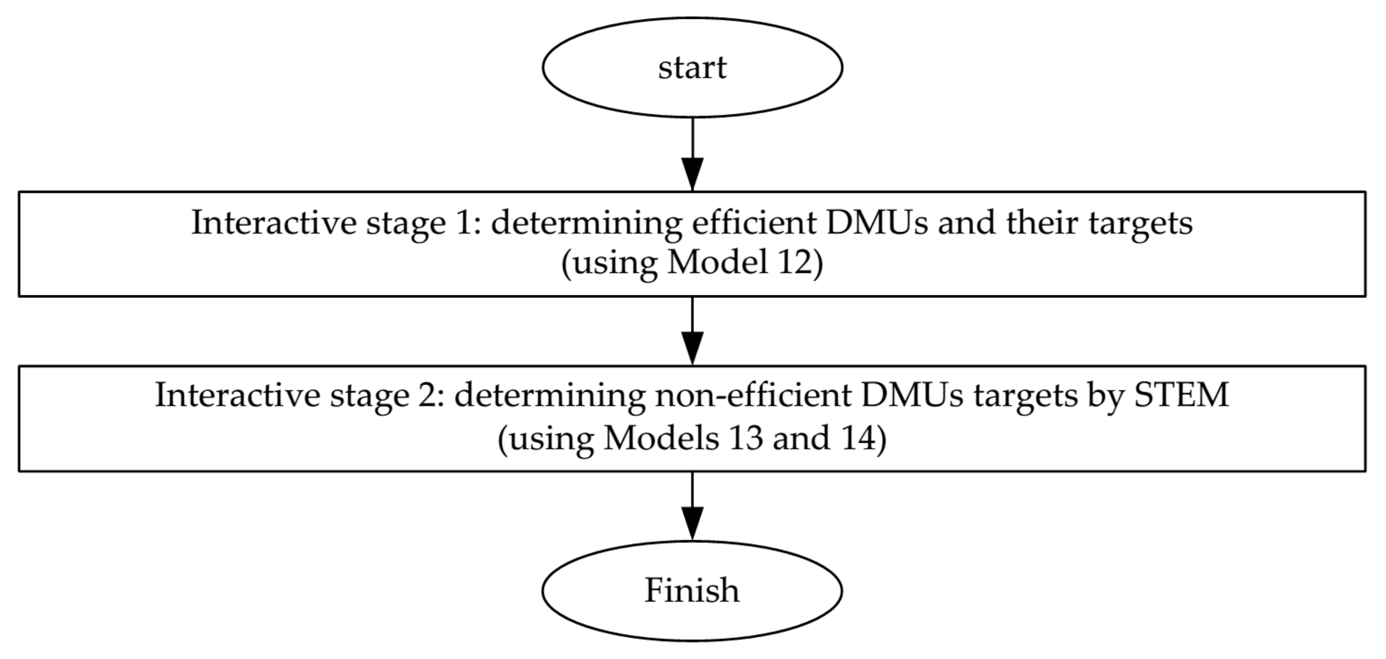
The brief of the interactive algorithm for finding DMU targets is shown in
Figure 1. In the interactive stage 1, efficient DMUs and their targets are determined. It is remarkable that by applying the first interactive stage of the interactive algorithm, at least one DMU
j, j = 1, …, n is efficient (at least, one member belongs to M set). The number of
set members are determined by composing and solving of non-radial model 12 for all DMUs. The required number of iterations for the interactive algorithm depends on the number of
set members. Non-radial model 12 should be constructed and solved n (number of DMUs) times. If the ratio of “the number of
set members” to “all DMUs” is near to 0, the interactive algorithm needs lesser iterations. If this ratio is near to 1, the interactive algorithm needs more iterations. In the interactive stage 2, non-efficient DMUs targets are determined using STEM.
The required times to construct and find targets of non-radial model 13 (step 0 of STEM) are equal to the number of set members. The required times to construct and find targets of non-radial model 14 (steps 1 and 2 of STEM) is dependent on DM’s opinions about the suitable target for each considered DMUo. The required iteration number to apply the second interactive stage is equal to the number of set’s members, which is defined the first time. As the number of set’s members is less than n (because at least, one member belongs to M set and set is defined as in the first interactive stage), the targets of all DMUs are therefore found in less than n iterations applying the second interactive stage of the interactive algorithm. This means that the interactive algorithm is completed by applying the second interactive stage in less than n iterations.
It is considerable that finding DMU targets of three kinds of non-radial FDH models (models 12–14) is required in the first part of hybrid technique. These targets can be found by solving related non-radial FDH models. RBA is one of the suitable methods to find DMU targets of radial FDH models, without solving of any mathematical models. In the second part of the hybrid technique, extended RBA is proposed to find DMU targets of non-radial FDH models without solving any mathematical models.
3.2. Extended RBA
In this section, extended RBA (the second part of proposed hybrid technique) to find DMU targets in non-radial FDH models of the interactive algorithm is described. As described in
Section 3.1, finding DMU targets of three non-radial FDH models of the interactive algorithm (models 12–14) are required. All mentioned models are mixed 0–1 LP and finding DMU targets by solving them is difficult. RBA can find DMU targets of radial FDH models without solving them. Only non-radial model 12 has a lot of similarity to radial FDH models (models 7 and 8). Therefore, finding DMU targets of non-radial model 12 may be possible using RBA with a little modification. However, RBA cannot apply to find DMU targets of non-radial FDH models 13 and 14, because these models have some complicated constraints. In this section, extended RBA is proposed to find DMU targets of non-radial FDH models without solving any mathematical programming models.
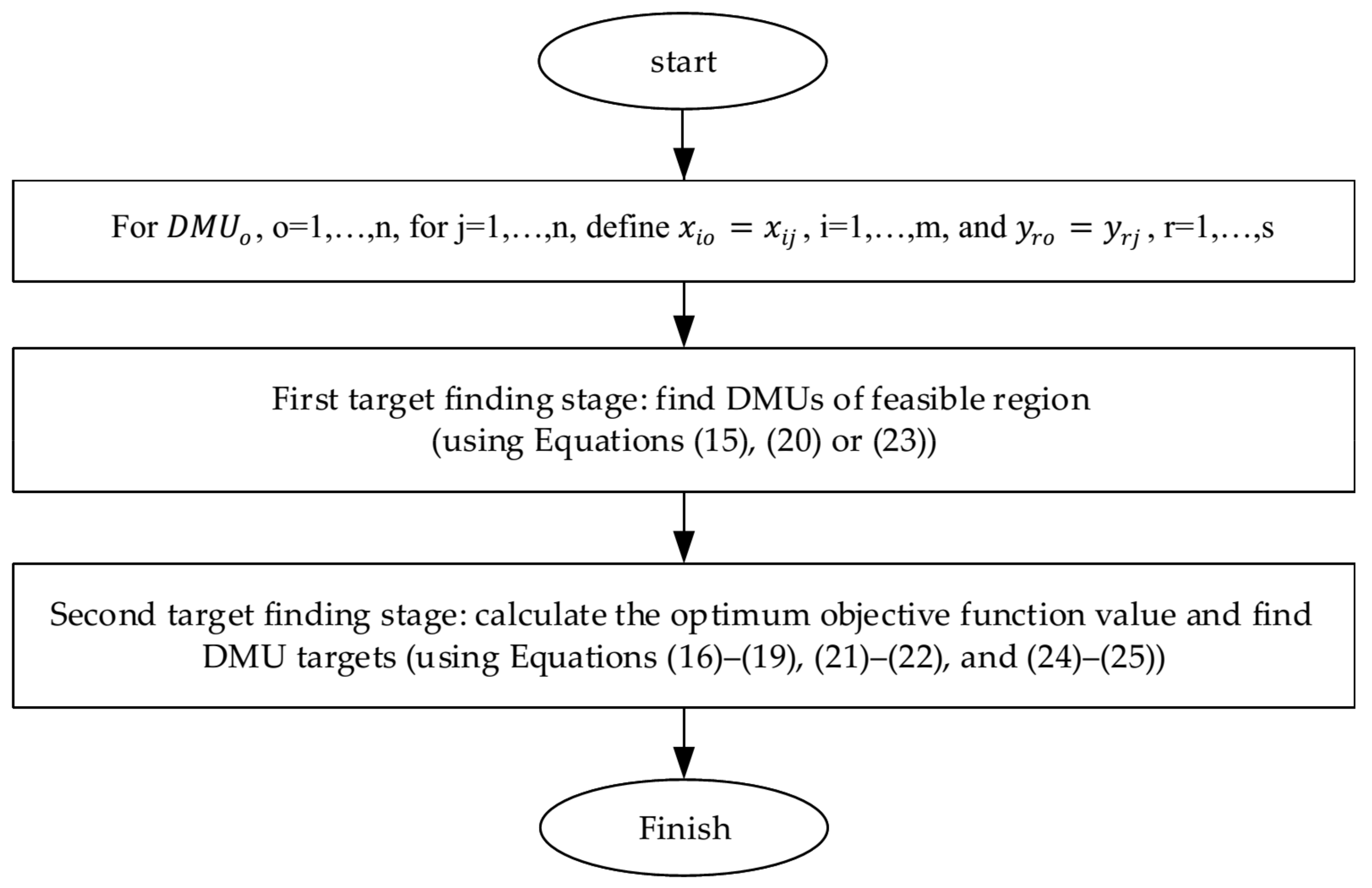
Define and for , o = 1, …, n, for j = 1…n. The extended RBA then find DMU targets of non-radial FDH models of the interactive algorithm (models 12–14) through two target finding stages. In the first target finding stage, DMUs of feasible region are found. In this regard, DMUs that have one, two or three conditions are considered as DMUs of feasible region. The number of required conditions for this stage depends on the constraints of the model. The first condition of extended RBA is similar to RBA and can be applied for non-radial FDH models 12–14. The second and third conditions are applied for non-radial model 14. In the second step, the optimum objective function value is calculated and DMU targets are found. Extended RBA are described in the following subsections.
3.2.1. Finding DMU Targets of Non-Radial FDH Models 12 and 13
As the constraints of non-radial FDH models 12 and 13 are exactly the same, finding DMU targets of these models are described simultaneously.
First, DMUs of feasible region should be found. Similar to RBA, if the constraints
and
are satisfied for DMU
j, j = 1, …, n (the first condition), DMU j, j = 1, …, n belongs to
. So, the DMUs of feasible region of non-radial FDH models 12 and 13 are determined using Equation (15).
As mentioned above, the first condition of extended RBA is similar to RBA.
The optimum objective function values should be calculated and DMU targets should be found in the second target finding stage. To achieve this, the objective function value of each DMU
j, j = 1, …, n in
(in non-radial model 12,
and in non-radial model 13,
) is calculated. The maximum obtained value for DMUs belonging to
, shows optimum objective function value (the optimum objective function value of non-radial FDH models 12 and 13 are
and
, respectively). Therefore, the optimum objective function values of non-radial FDH models 12 and 13 are calculated by Equations (16) and (17), respectively.
Then, the DMUs of
which have optimum objective function value show the targets of
in each model. Therefore, DMU
o targets in non-radial FDH models 12 and 13 are determined by Equations (18) and (19), respectively.
As described in
Section 3.1, both steps 1 and 2 of STEM’s model are shown by non-radial model 14. Finding DMU targets of related non-radial FDH models by extended RBA are described in
Section 3.2.2 and
Section 3.2.3.
3.2.2. Finding DMU Targets of Step 1 of STEM’s Model
The process of applying extended RBA to find DMU targets of step 1 of STEM’s model is described in two target finding stages as follows:
In the first target finding stage, finding DMUs of feasible region (in step 1 of STEM model) is desired. In DMUs of feasible region (DMU
j, j = 1, …, n), two conditions should be satisfied. Firstly, in these DMUs, similar to non-radial FDH models 12 and 13, constrains
, i = 1, …, m, and
, r = 1, …, s should be satisfied for DMU
j, j = 1, …, n. The method of checking this condition for DMUs of feasible region (DMU
j, j = 1, …, n) has been described in
Section 3.2.1. Secondly, in DMUs of feasible region, the constraint
should be satisfied for DMU
j, j = 1, …, n. In constraints of the second condition, the values of
and
are obtained from solving non-radial model 13 and calculated using Equation (4), respectively. For checking the second condition,
and
are calculated for DMU
j, j = 1, …, n that were compatible in the first condition. Then constraints
are checked for mentioned DMUs. In DMUs belonging to the feasible region of non-radial model 14 (step 1 of STEM), in addition to the first condition, constraints
should be satisfied for j = 1, …, n (the second condition), too. In DMUs of feasible region, the first and second conditions should be satisfied in DMU
j, j = 1, …, n, simultaneously. Therefpre, the DMUs of
are determined using Equation (20).
The optimum objective function values of step 1 of the STEM model should be calculated and DMU targets of the model should be found in the second target finding stage. The optimum objective function value of step 1 of STEM model is calculated by Equation (21).
After that, the DMUs of
which have optimum objective function value shows the targets of
in the model. Therefore, the DMU
o targets in step 1 of STEM are determined using Equation (22).
3.2.3. Finding DMU Targets of Step 2 of STEM’s Model
Finding the optimum solutions of non-radial model 14 (step 2 of STEM), without solving any mathematical models, is described in two target finding stages below.
First, DMUs of feasible region in step 2 of the STEM model should be found. In DMUs of feasible region, three conditions should be regarded. The first and second conditions should be tested for DMU
j, j = 1, …, n as described in
Section 3.2.2, but in the second condition,
should be determined again. The third condition relates to
and
constraints that
are obtained from suggested target of DM. So in DMUs of feasible region, constraints
and
for j = 1, …, n should be satisfied, too. So, the selected DMU
j of
set are defined as Equation (23).
The optimum objective function value of step 2 of the STEM model should be calculated and DMU targets of mentioned model should be found in the second target finding stage. The optimum objective function value of step 1 of the STEM model is calculated by Equation (24).
After that, the DMUs of feasible region which have optimum objective function values show the targets of
in the model (Equation (25)).
It is remarkable that
exists, if the best compromise solution is found in step 2 of the STEM model (
Section 3.1). The brief of applying extended RBA to find non-radial FDH models targets of the interactive algorithm is shown in
Figure 2.
4. Two Real Case Studies
The proposed technique was applied in two real case studies. The description is provided in
Section 4.1 and
4.2.
4.1. The First Case Study: University Departments
The data set of 17 university departments of Islamic Azad University of Mobarakeh Iran (mobarakeh.iau.ir), denoted by DMU
01, …, DMU
17, were extracted from reported research [
39]. These data were also used by another study [
15]. Each DMU
j, j = 1, …, 17 has two inputs and two outputs.
The names of inputs are “the number of bachelor students” and “the number of (full time and part time) faculty members”. The names of outputs are “the number of graduates” and “the number of research papers”. The data of the first case study are shown in
Table 2.
As mentioned previously, in DEA models, choosing appropriate inputs, outputs, and DMUs is an important subject. In this case study, the relationship existed ()).
4.1.1. Applying the Interactive Algorithm for the First Case Study
To find DMU targets, the interactive algorithm (
Figure 1), including two interactive stages, was applied for universities departments.
In this stage, efficient DMUs and their targets were determined. For o = 1, …, 17, parameters
, j = 1, …, 17, and
were defined. Non-radial model 12 was then composed for
. The results of solving of model 12 for
are shown in
Table 3.
Considering
Table 3,
and
were defined. Then
,
was also defined. So, obtained results from 17 times (number of DMUs) composing and solving non-radial model 12 (the first interactive stage) showed that 14 DMUs lay on the efficient frontier, and 3 DMUs did not. By applying the second interactive stage, the DMU targets of these three DMUs were distinguished.
In the second interactive stage, the targets of DMUs belonging to set
were found by STEM. First, the pay-off tables for non-proceed DMUs were constructed. As
(
has 3 members), the interactive algorithm (
Figure 1) should be continued to find targets of
set considering
, one by one. But here, the process of applying the interactive algorithm for
,
and
are described simultaneously. So, each of these three DMUs
was considered as a non-proceed DMU that their targets should be defined.
Firstly,
, j = 1, …, 17, and
were defined for DMU
o, o = 5,6, and 16. Then the pay-off tables (
Table 4) were constructed by composing and solving of model 13 for
l = 1, …, 4. In model 13, n = 17 and m = s = 2 are considered for each DMU
o, o = 5, 6, and 16.
It is mentionable that the required times to construct and solve model 13 in the interactive algorithm were equal to 3 (the number of
set members). In this interactive stage, finding a suitable DMU in feasible region as the target of
, o = 5, 6, and 16 was desired which the value of f
l, l = 1, …, 4 was as good as the suggested
target, o = 5, 6, and 16 by DM. Supposed that the targets of
,
and
according to DM’s opinions were
,
and
, respectively. So, suggested targets of DM were considered as DM’s opinions for f
l, l = 1, …, 4. After that, the first iteration of STEM (p = 1) was started. In step 1 of STEM (calculation phase), first
was calculated by Equation (4) considering
Table 4, then
,
was calculated as shown in
Table 5.
Then model 14 for
,
and
(Step 1 of STEM for p = 1) were composed. The results of solving these models and DM’s opinions about them are shown in
Table 6. As seen in the last column of
Table 6, the targets of
,
and
via solving of model 14 (Step 1 of STEM for p = 1) were
,
and
, respectively.
As described previously, these targets were acceptable according to DM’s opinion, too. As the obtained solutions for and were satisfied via DM’s opinions, the best compromise solutions were obtained for these DMUs.
Then,
(
) from
set removed (
(
has 1 member). As the value of the fourth target of
was not satisfied via DM’s opinions, the obtained solution was not the best compromise solution. So, composing model 14 related to Step 2 of STEM (p = 1) was required for
. The required parameters were calculated as shown in
Table 7.
Non-radial model 14 for
was then composed for the first iteration of step 2 of STEM. The results of solving this model showed that there was only one similar unsatisfied objective function (fourth objective function) in two consecutive steps of STEM. Therefore, the target of
could not be considered as
. Therefore, the interactive algorithm was continued by asking DM to suggest a new target for each DMU
o. DM did not suggest new DMUs target for
so there were no targets for
in the FDH model. Then,
(
) from
set was removed (
). As there was no non-proceed DMUs and the process of targets determination for all DMUs had been carried out (
), the interactive algorithm was finished. The results of applying the interactive algorithm for all DMUs are shown in
Table 8.
As shown in the last column of
Table 8, applying the interactive algorithm for university departments are considered as three cases.
were members of M set and the targets of these DMUs were themselves (case 1). As best compromise solutions were found through step 1 of STEM for
,
, these DMUs belonged to case 2. As there was only one similar unsatisfied objective function in two consecutive steps of STEM for
, this DMU belonged to case 3.
It should be mentioned that in the first case study, 14 DMUs from 17 DMUs (about 82%) lay on the efficient frontier. Moreover, non-radial FDH models 13 and 14 were composed and solved, three and four times through the second interactive stage, respectively. Here, the process of target determination for all DMUs was carried out, and the interactive algorithm finished. In fact, the required repetition times for composing and solving non-radial model 14 depend on DM’s opinions about suitable targets for each considered DMUo.
4.1.2. Applying Extended RBA for the First Case Study
As described in
Section 4.1.1, for applying the interactive algorithm for the first case study, solving of non-radial FDH models 12, 13, model 14 of step 1 of STEM (p = 1), and model 14 of step 2 of STEM (p = 1), 17, 3, 3, and 1 times were needed, respectively. So, solving 24 mixed 0–1 LP models were required to find all DMU targets. The DMU targets of mentioned non-radial FDH models could be found using extended RBA through two target finding stages without solving any mathematical programming models. In this section, applying extended RBA for finding DMU targets of these non-radial FDH models (models 12–14 for DMU05 of university departments) are described. First
and
(j = 1, …, 17) were defined for
= DMU
05 (
Figure 2).
Target finding of non-radial FDH models 12 and 13 for DMU05 in the first case study
In this regard, DMUs of feasible region should be found in applying the first target finding stage. Firstly, DMUs of feasible region (
) should be found using Equation (15) (
Figure 2). In DMUs of feasible region, constraints
and
(j = 1, …, 17) should be satisfied. The results of checking constraints of the first condition are shown in
Table 9. As it is observed in the last column of
Table 9, only DMU
03 and DMU
05 satisfied all four constraints of the first condition. So,
.
The optimum objective function values and DMU targets should then be found in applying the second target finding stage. At first, the optimum objective function values of models should be calculated by Equations (16) and (17) (
Figure 2). The objective function values of DMU
03 and DMU
05 (in model 12,
, and in model 13,
) are shown in
Table 10.
The last row of
Table 10 shows the maximum values of
,
and
, respectively. These values show the optimum objective function value of each model (
). The
targets were then found by comparing the optimum objective function values of each model with the objective function value of each DMU by Equations (18) and (19) (
Figure 2). It is considerable that non-radial model 13 with
objective function had alternative solutions.
First, step 1 of STEM (p = 1) should be considered. DMUs of feasible region (in step 1 of STEM model) should be found through applying the first target finding stage. First, DMUs belonging to the feasible region should be found. In DMUs of feasible region, two conditions should be satisfied. Firstly, constraints
and
(j = 1, …, 17) should be satisfied (the first condition). As it is seen in
Table 9, only DMU
03 and DMU
05 satisfied these constraints. Moreover, the constraints
should be satisfied for each DMU of feasible region (the second condition). Checking the second condition for DMU
03 and DMU
05 are shown in
Table 11.
As seen in
Table 11, the constraints of the second condition were also satisfied for DMU
03 and DMU
05. So,
.
The optimum objective function value of step 1 of STEM model was then calculated, and DMU targets were found through applying the second target finding stage. With respect to Equation (21), the minimum values of the left-hand side of the second condition for DMU
03 and DMU
05 showed the optimum objective function value of non-radial model 14 (last row of
Table 11). As is seen in Equation (22), each DMU with an objective function value equal to the optimum objective function value, showed the targets of
. So, the target of DMU
05 was DMU
03, as seen in the last column of
Table 11 (
.
It is mentionable that the obtained results from target finding of all non-radial FDH models 12–14 for the first case study for DMU05 using extended RBA are the same as the results obtained from solving the mentioned mathematical models. Here, target finding of three non-radial FDH models of 24 mathematical programming models using extended RBA were described. A similar process should be undertaken to find targets of other 21 non-radial FDH models.
4.2. The Second Case Study: Operations Strategies of Fars Province Pharmaceutical Distributing Companies
By considering expert opinions, 13 active pharmaceutical distributing companies (Fars province of Iran) in 2019 were investigated. These companies were Daroo Pakhsh, Pakhshe Razi, Adora Teb, Mahya Daroo, Alborz, Hejrat, Daroo Gostare Razi, Behestan Pakhsh, Ghasem Iran, Yasin, Ferdos, Elit Daroo, and Soha Helal. The operations strategies of these companies denoted as DMU01, …, DMU13.
There are five generic performance objectives including cost, delivery speed, quality, dependability, and flexibility. Joining the market requirements through a beneficial method for operations is the purpose of these objectives. These objectives are applicable for different operations. Satisfaction of customers can be obtained through reaching these mentioned objectives [
40]. According to expert opinions, these five generic performance objectives were very important in the operation strategies of Fars province pharmaceutical distributing companies. In this regard, cost was defined as the lower cost for producing products and services, and decreasing the cost of distributing medicinal drugs and increasing customers are desirable for pharmaceutical distributing companies. Delivery speed was defined as an elapsed time between the beginning of an operations process and its end, and increasing trucks, vans, and motorcycles numbers could improve delivery speed. Quality was defined as fit-for-purpose, and comparing distributed medicinal drugs with orders and checking the temperature of transportation refrigerators could improve quality. Dependability was defined as keeping delivery promises and distributing medicinal drugs in the promised time and increasing transportation vehicles could improve dependability. Flexibility was defined as treating the operation as a ‘black box’ and considering the types of flexibility that would contribute to its competitiveness (product or service flexibility, mix flexibility, volume flexibility, and delivery flexibility) and having up to date information about existing medical drugs and having a powerful team to prepare them could improve flexibility.
As mentioned previously, in DEA models, choosing appropriate inputs and outputs is an important subject. As classical DEA models are based on decreasing inputs and increasing outputs, in operations strategies of Fars province pharmaceutical distributing companies, cost and delivery speed were considered as inputs that denoted by I1 and I2. Furthermore, quality, dependability, and flexibility were considered as outputs that were denoted by O1, O2 and O3. These inputs and outputs were relevant to the research area and expert(s) confirmed them. All DMUs in the research area were considered as DMUs. So, each DMUj, j = 1, …, 13 had two inputs (I1 and I2), and three outputs (O1, O2 and O3). As mentioned previously, establishing a relationship between inputs, outputs, and DMU numbers is recommended. Here, all DMUs in the research area were considered and increasing DMUs to reach exact relationship was impossible in a practical view (this relationship almost existed (). As we will see later, only two DMUs were efficient in the second case study. So, in this case study, decreasing the number of DMUs did not also create difficulty in the theoretical view.
As only experts accessed real data related to inputs and outputs of each DMU, expert judgement was used. With respect to each input and output, the performance of each DMU was scaled by 1 to 9 considering expert opinions (
Table 12). The data of inputs and outputs of operations strategies of Fars province pharmaceutical distributing companies (the second case study) are shown in
Table 13.
As the process of applying the hybrid technique for the second case study had a lot of similarity with the first case study, its main results are described in
Section 4.2.1 and
Section 4.2.2. The details of applying the method for the second case study are shown in
Appendix A.
4.2.1. The Main Results of Applying the Interactive Algorithm for the Second Case Study
To find DMU targets for the second case study, the interactive algorithm, including two interactive stages (
Figure 1), was applied. In applying the first interactive stage (
Appendix A,
Appendix A.1), non-radial model 12 was composed and solved 13 times. The results show that only 2 DMUs (about 15%) lay on the efficient frontier, and 11 DMUs did not (
Appendix A,
Table A1). By applying the second interactive stage (
Appendix A,
Table A2,
Table A3,
Table A4,
Table A5 and
Table A6), DMU
07 target was obtained, but DMU
04 and DMU
10 target were not obtained. The brief results of applying the interactive algorithm (
Figure 1) for all DMUs are shown in
Table 14.
As seen in the last column of
Table 14, applying the interactive algorithm for the second case study can be categorized into four cases. As shown in
Table 14, DMU
01 and DMU
06 are members of M set and the target of these DMUs are themselves (case 1). The obtained targets by solving step 1 of the STEM model and via DM’s opinions of DMU
02, DMU
03, DMU
05, DMU
07, DMU
09, and DMU
11 are DMU
01. By applying step 1 or 2 of STEM, the best compromise solutions for these DMUs are found (DMU
01) via DM’s opinions (case 2). By solving step 1 of the STEM model, DMU
01 is obtained as the target of the rest DMUs. But the target of these DMUs via DM’s opinions are DMU
06 (case 3 and 4). For DMU
04, DMU
08, and DMU
13, a compromise solution is not found because there is only one similar unsatisfied objective function in step 1 and the first iteration of step 2 of STEM (case 3). The best compromise solution is not obtained for DMU
10 because
, l = 1, …, 5 is not calculable for the first iteration of step 2 of STEM (case 4). The required repetition times of composing and solving non-radial model 14, depends on DM’s opinions about suitable target for each considered DMU
o. In
Appendix A, finding the target of a DMU in each case are described.
4.2.2. The Main Results of Applying Extended RBA for the Second Case Study
As described in
Appendix A.2 (
Appendix A), through applying the interactive algorithm for the second case study, non-radial FDH models 12, 13, non-radial FDH model 14 of step 1 of STEM (p = 1), and non-radial model 14 of step 2 of STEM (p = 1) should be solved 13, 11, 11, and 5 times, respectively. So, finding targets of 40 mixed 0–1 LP models were required. The target of these non-radial FDH models could be obtained using extended RBA through two target finding stages (
Figure 2). In
Appendix A.2, applying extended RBA for solving three of these non-radial FDH models (models 12–14 for DMU
05 of the second case study) are described.
The detail results of applying extended RBA (
Figure 2) to solve non-radial FDH models 12–14 for DMU
07 of the second case study (related non-radial FDH models in the interactive algorithm) are described in
Appendix A.2 (
Appendix A). Each target of model was found using two target finding stages for DMU
07 of the second case study considering related conditions.
and
(j = 1, …, 13) were firstly defined for
= DMU
07.
Applying extended RBA for non-radial FDH models 12 and 13 (
Appendix A,
Appendix A.2), showed that
and some non-radial FDH models had alternative targets. Applying extended RBA for non-radial FDH model 14 (
Appendix A,
Appendix A.2), showed that
and DMU
01 was the only target (
Table A9).
By solving step 1 of the STEM model (non-radial FDH model 14), DMU
01 was obtained as the DMU
07 target (
Appendix A,
Table A10). However, the obtained target via DM’s opinions was DMU
06. A compromise solution was not found because no feasible integer solution could be found in the first iteration of step 2 of STEM.
It is mentionable that the results obtained from solving of all non-radial FDH models 12–14 for the second case study DMU
07 using extended RBA were the same as the results obtained from solving of mentioned models using regular approaches. As described in
Appendix A.2 (
Appendix A), solving three models of 40 non-radial FDH models were described. A similar process should be undertaken to solve other 37 mathematical models.
As mentioned previously, the suggested hybrid technique contains the interactive algorithm (the first part) and extended RBA (the second part). The interactive algorithm contains two stages. In the interactive stage 1, inputs, outputs, DMUs, and then efficient DMUs and their targets are determined. According to the proposed technique, using real data is preferred rather than gathering them from experts’ opinions. In the first case study, inputs, outputs, and DMUs information were real and extracted from a published paper. In the second case study, only experts accessing the real data related to inputs and outputs of each DMU. So, experts’ judgements, in situations where experts accessed real data, were used. The number of set members are determined by composing and solving non-radial model 12 for all DMUs. The required number of iterations for the interactive algorithm depends on the number of set members. Non-radial model 12 should be constructed and solved n (number of DMUs) times. It is considerable that the number of DMUs in the first and second case studies are 17 and 13, respectively. If the ratio of “the number of set members” to “all DMUs” is near to 0, the interactive algorithm needs fewer iterations. If this ratio is near to 1, the interactive algorithm needs more iterations. As it is found for applying the first interactive stage in the first case study, if the number of DMUs that lie on the efficient frontier is considerable (14 DMUs from 17 DMUs, about 82%), the interactive requires fewer iterations. However, as it is found for the second case study, if the number of DMUs that lie on the efficient frontier of model 12 is not considerable (2 DMUs from 13 DMUs, about 15%), the interactive algorithm requires more iterations.
In the interactive stage 2, non-efficient DMUs targets are determined using STEM. The required times to construct and find targets of model 13 (step 0 of STEM) are equal to the number of set members. The number of set members in the first and second case studies were 3 and 11, respectively. The required time for constructing and finding targets of model 14 (steps 1 and 2 of STEM) is dependent on DM’s opinions about a suitable target for each considered DMUo. These numbers in the first and second case studies were 3 and 11, respectively. Therefore, by applying 3 and 11 times of interactive stage 2, the process of targets determination for non-efficient DMUs of the first and second case studies was carried out, respectively, and the interactive algorithm finished. Moreover, solving 24 and 40 non-radial FDH models were required in the first and second case study, respectively.
5. Conclusions
Finding DMU targets or DMU projections is useful for strategic planning in some organizations. In these organizations, a convexity assumption does not exist, and decisions are made on the basis of pareto solutions. Therefore, these properties should be considered in practical models. Moreover, by eliminating the convexity assumption, FDH models can be applied. As suggesting a technique with mentioned properties has been neglected in previous research, the main novelty of this paper is in its suggestion of this technique. In this regard, the answers to the two research questions are as follow:
- (a)
Is it possible to propose a technique to find all DMU targets in non-radial FDH models based on ASBM using IM? Using IMs such as STEM to find DMU targets in non-radial FDH models on the basis of slack variables can be an important subject and it is applied in the proposed technique.
- (b)
Is it possible to find DMU targets of non-radial FDH models in the proposed technique without solving any mathematical models? In this research, in addition to using STEM for finding DMU targets in non-radial FDH models, DMU targets of non-radial FDH models were found by extended RBA without solving any mathematical models.
As has been explained previously, after determining inputs, outputs and DMUs in the first and second case studies, four DMUs from 17 DMUs (76% of DMUs) and two DMUs from 13 DMUs (15% of them) lay on the efficient frontier, respectively. So, in applying the second interactive stage for the first and second case studies, 76% and 20% of DMUs could be selected as targets, respectively. Moreover, the targets of all non-radial FDH models were found using extended RBA without solving any mathematical programming model. In fact, the obtained results can be extended to other cases considering practical and theoretical views.
As mentioned previously, using real data related to inputs, outputs, and DMUs is preferred rather than gathering them from experts’ opinions according to the proposed technique. However, if gathering real data was impossible, experts’ judgement would be used. In this situation, experts should access real data or have enough information about the problem. The existence of, and access to, such experts can be considered as the first limitation of this study. We assumed that there are no outliers, and this assumption can be considered as the second limitation of this research. Furthermore, all required data existing in deterministic form can be considered as the third limitation of this study.
Detecting outliers and investigating the sensitivity of the modeling approach to outliers in the proposed technique, finding DMU targets using other IMs, using impressive data in supply chain management, and adopting the proposed technique in situations where data are fuzzy can be considered as future studies.


