Simulation of Wood Combustion in PATO Using a Detailed Pyrolysis Model Coupled to fireFoam

Abstract

The numerical simulation of fire propagation requires capturing the coupling between wood pyrolysis, which leads to the production of various gaseous species, and the combustion of these species in the flame, which produces the energy that sustains the pyrolysis process. Experimental and numerical works of the fire community are targeted towards improving the description of the pyrolysis process to better predict the rate of production and the chemical nature of the pyrolysis gases. We know that wood pyrolysis leads to the production of a large variety of chemical species: water, methane, propane, carbon monoxide and dioxide, phenol, cresol, hydrogen, etc. With the idea of being able to capitalize on such developments to study more accurately the physics of fire propagation, we have developed a numerical framework that couples a detailed three-dimensional pyrolysis model and fireFoam. In this article, we illustrate the capability of the simulation tool by treating the combustion of a wood log. Wood is considered to be composed of three phases (cellulose, hemicellulose and lignin), each undergoing parallel degradation processes leading to the production of methane and hydrogen. We chose to simplify the gas mixture for this first proof of concept of the coupling of a multi-species pyrolysis process and a flame. In the flame, we consider two separate finite-rate combustion reactions for methane and hydrogen. The flame evolves during the simulation according to the concentration of the two gaseous species produced from the material. It appears that introducing different pyrolysis species impacts the temperature and behavior of the flame.

1. Introduction

Charring materials (timber and composite materials) are widely used in many civil [1] and aeronautical [2] applications. On the one hand this leads to a sustainable development with lower energy requirements and less pollution, but on the other hand, this may lead to fire hazards. These materials have a flammable nature, and this makes necessary the prediction of a fire potential with the consequent loss of stiffness, strength and resistance of a structure [3]. In the recent few decades, different studies approached the topic and aimed to characterize the performance of charred materials under combustion. Fire retardancy [4], flammability properties [5] and gaseous emissions [6] are just a few examples of the main properties that have been studied. The main strength of this fire community lies in its ability to describe how a fire behaves for a given material, including the description of ignition, fire growing, propagation and extinction processes [7]. Different numerical simulation programs have been developed for such purposes. One of the most successful is fireFoam [8], an opensource code to simulate and visualize the fire behavior in a defined geometry. Different application cases can be found in the literature [9,10,11].

In a numerical simulation, modeling the flame is not enough. A description of the charred material degradation process in the absence of oxygen (the pyrolysis), as well as the coupling between material and environment, are fundamental aspects that need to be captured. Pyrolysis leads to the production of a large variety of chemical species: water, methane, propane, carbon monoxide and dioxide, phenol, cresol, hydrogen, etc. The production of these species and their concentration is strongly affected by the imposed conditions [12,13]. This would not affect only the material, but even the combustion process. The gaseous species, once produced, will percolate in the material and eventually reach the external environment. Many of these species are fuels, therefore the correct prediction of their formation could change the outcome of the simulation. Different pyrolysis models have been developed during the years, each characterized by a different level of accuracy in the description of the chemical reactions. The simplest one is the single reaction mechanism [14] in which only a single decomposition reaction is considered. A next step is done with the multi-component single reaction model [15] where the description becomes sensible to the feed-stock. With an increase in complexity, there is the competitive model [16] that introduces competitive reactions to predict different product distributions depending on the conversion conditions, such as heating rate and pressure. Finally, there are the competitive multi-component models [17,18] which represent efficiently the dependence on the feed-stock as well as the temperature effect on the yields.

Pyrolysis is not the only process to model in charring materials. Mass, momentum and energy of the material need to be conserved, and the transport of gaseous species also need to be taken also into account. A generic combustion problem with a charring material is schematized in Figure 1.

The problem may be split in two regions: the environment, where combustion happens, and the material, characterized by a thermal degradation process, the pyrolysis. Two different models are required for the numerical resolution. We chose to couple fireFoam with a detailed pyrolysis model. The latter enters in the type-3 models classification proposed by Lachaud et al., 2011 [19], and it has already been applied to different applications, like ablative heat-shield design and pyrolysis of lignocellulosic biomass [20,21,22].

The main objective of this paper is to propose for the first time a numerical framework that couples a detailed three-dimensional pyrolysis model and fireFoam. The numerical framework with the description of the two numerical models is given in the next sections: Section 2 presents the detailed pyrolysis model and Section 3 presents the combustion process. The coupling conditions between the two models are given in Section 4. The capabilities of the solver are showed in Section 5, where two different applications are considered. The first one aims to show how the introduction of different pyrolysis species impacts the temperature and the behavior of the flame. The second application is a 2D simulation of a wood log combustion. Here, we chose to simplify the gas mixture for this first proof of concept of coupling of a multi-species pyrolysis process and a flame. Results show a perfect coupling between the two models and highlight the impact of the species, whose concentration change in time, on the fire behavior. Finally, conclusions are drawn in Section 6.

2. Numerical Model: Material Region

The model to describe the material region is presented in this section. It consists of a generic pyrolysis model that allows the description of the interaction between several solid phases and a gas phase [22]. A summary of the governing equations of the solid phases, gas and species are presented in the following subsections.

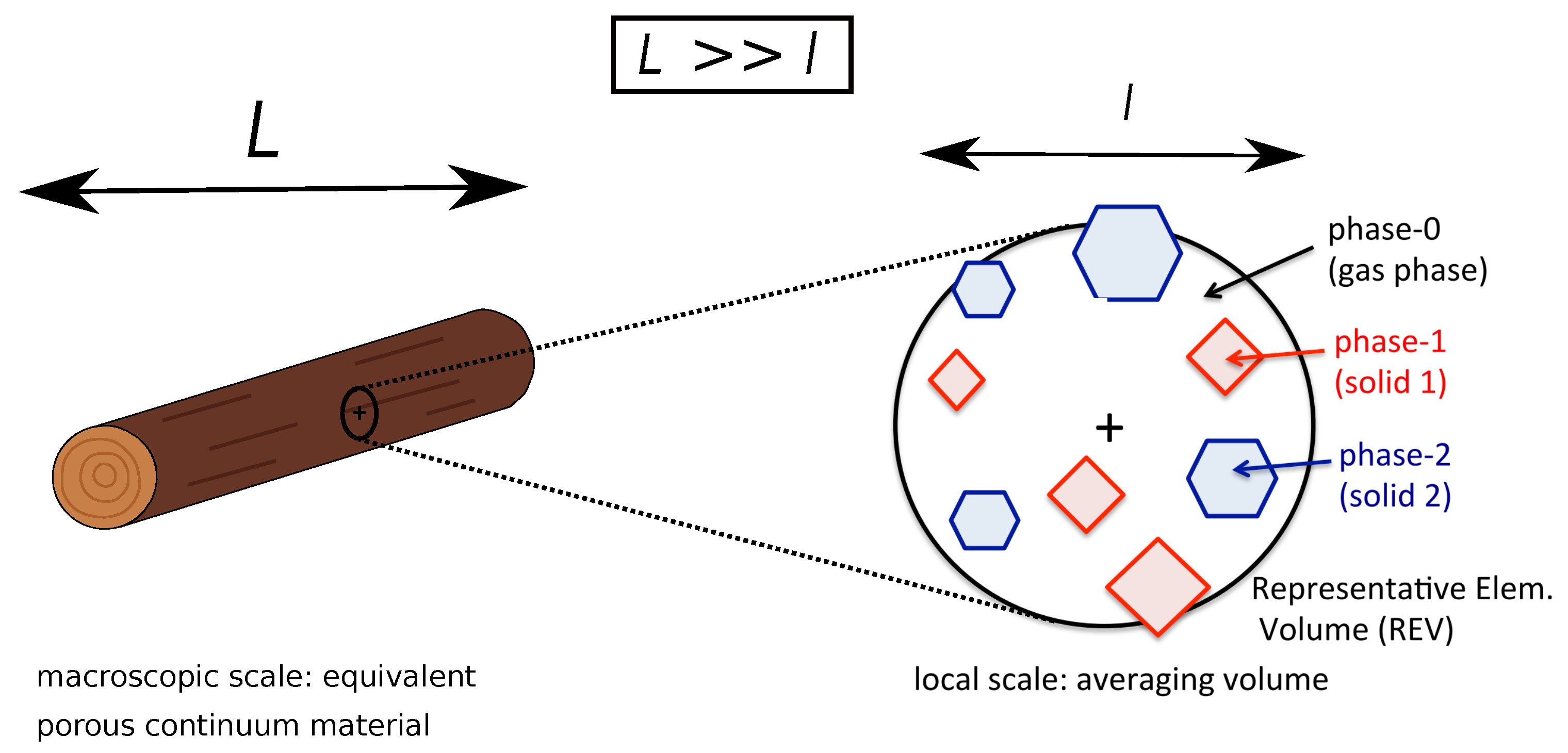
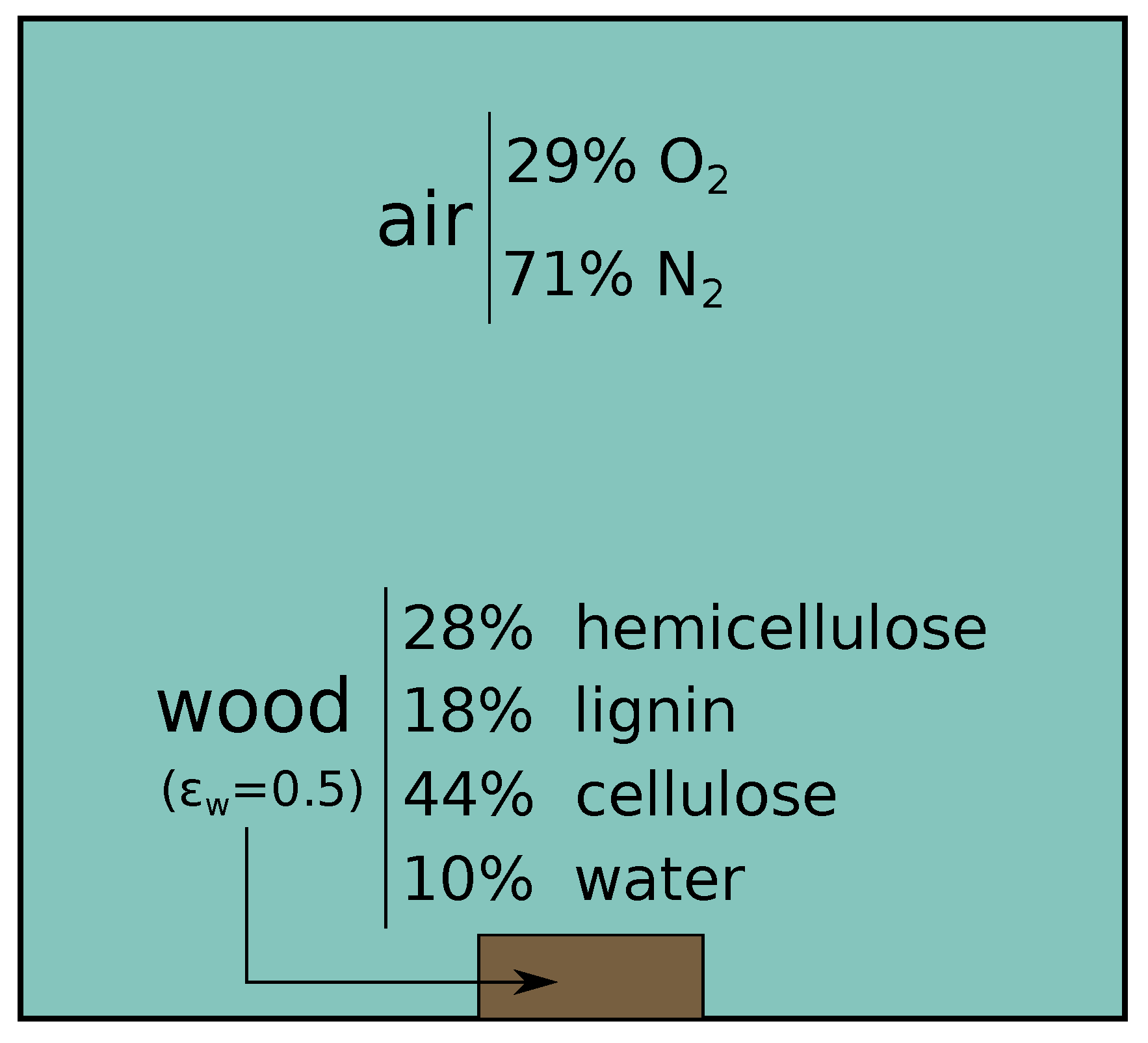
2.1. Main Assumptions

The model considers the interaction between a multi-phase reactive material ($N_p$ solid phases) with a multi-species reactive gas mixture ($N_g$ gaseous elements/species). No liquid phase is modeled. Any liquid present in the material (water) is modeled as a solid phase. The description is done at the macroscopic scale, where the governing equations can be derived from upscaling theories. Their derivation relies on the existence of a representative elementary volume (REV) of the domain and on the assumption of scales separation, as illustrated in Figure 2.

2.2. Pyrolysis

The material is assumed to be composed of $N_p$ solid phases. For example, in the wood-cell walls the main components are cellulose, hemicellulose, and lignin, which are modeled as three phases. Each solid phase $s_i$ may decompose following several pyrolysis kinetics in the absence of oxygen. For this reason, each phase i is split into $P_i$ sub-phases to model the different degradation mechanisms. A generic decomposition of a sub-phase j (from solid phase i) leads to the production of species $A_k$ according to the stoichiometric coefficients ${\xi }_{i,j,k}$ as follows

$$s_{i,j}⟶\sum _{k=1}^{N_g}{\xi }_{i,j,k}{A}_k,\forall i\in [1,N_p],\forall j\in [1,P_i]$$

(1)

where $N_g$ is the total number of the gaseous species accounted for in the gas mixture. Pyrolysis reactions are modeled by Arrhenius laws. In this way, the advancement of the pyrolysis reaction ${\chi }_{i,j}$ of sub-phase j within phase i can be defined as

$${\partial }_t{\chi }_{i,j}={(1-{\chi }_{i,j})}^{m_{i,j}}{T}_g^{n_{i,j}}{\mathcal{A}}_{i,j}exp\left(-{\displaystyle \frac{{\mathcal{E}}_{i,j}}{R{T}_g}}\right),\forall i\in [1,N_p],\forall j\in [1,P_i]$$

(2)

where R is the perfect gas constant, $T_g$ the temperature of the gas, $\mathcal{A}$ the Arrhenius law pre-exponential factor, $\mathcal{E}$ the Arrhenius law activation energy, and m and n the Arrhenius law parameters. The total advancement in the pyrolysis process, $\tau$, is evaluated as follows

$$\tau =\sum _{i\in [1,N_p]}\sum _{j\in [1,P_i]}{\displaystyle \frac{{ϵ}_{i,0}{\rho }_{i,0}{F}_{i,j}}{{\sum }_{i\in [1,N_p]}{\sum }_{j\in [1,P_i]}{ϵ}_{i,0}{\rho }_{i,0}{F}_{i,j}}}(1-{\chi }_{i,j})$$

(3)

where ${ϵ}_i$, ${\rho }_i$, and $F_{i,j}$ denote, respectively, the volume fraction of phase i, the intrinsic density of phase i and the mass fraction of sub-phase j within phase i. The subscript 0 indicates the initial time ($t=0$).

The total production rate of species ${\pi }_k$ is given by

$${\pi }_k=\sum _{i\in [1,N_p]}\sum _{j\in [1,P_i]}{\xi }_{i,j,k}{ϵ}_{i,0}{\rho }_{i,0}{F}_{i,j}{\partial }_t{\chi }_{i,j}$$

(4)

By summing all the contributions in the gas mixture, it is possible to obtain the overall pyrolysis-gas production rate

$$\mathsf{\Pi }=\sum _{k\in [1,N_g]}{\pi }_k$$

(5)

2.3. Mass Conservation

We assume no heterogeneous reactions between the gaseous species and the solid phase. The only production terms come from the pyrolysis.

All the solid phases, the species, and the gas mixture should be taken into account. Each of them is characterized by a different mass conservation equation. For the solid phases, the equation reads

$$-{\partial }_t\left({ϵ}_i{\rho }_i\right)=\sum _{j\in [1,P_i]}{ϵ}_{i,0}{\rho }_{i,0}{F}_{i,j}{\partial }_t{\chi }_{i,j}$$

(6)

For a generic specie with mass fraction $y_i$, the conservation equation is

$${\partial }_t\left({ϵ}_g{\rho }_g{y}_i\right)+{\partial }_x·\left({ϵ}_g{\rho }_g{y}_i{v}_g\right)+{\partial }_x·F_i={\pi }_i,\forall i\in N_g^s$$

(7)

For the gas phase, the mass conservation needs to take into account the pyrolysis production rate. The term is added on the right hand-side

$$-{\partial }_t\left({ϵ}_g{\rho }_g\right)+{\partial }_x·\left({ϵ}_g{\rho }_g{v}_g\right)=-\sum _{i\in [1,N_p]}{\partial }_t\left({ϵ}_i{\rho }_i\right)=\mathsf{\Pi }$$

(8)

where $v_g$ is the averaged gas velocity.

2.4. Momentum Conservation

The average gas velocity is obtained from the Darcy’s law

$$v_g=-{\displaystyle \frac{1}{{ϵ}_g{\mu }_g}}\underline{\underline{\mathit{K}}}·{\partial }_x{p}_g$$

(9)

where $\underline{\underline{\mathit{K}}}$ is the permeability tensor and $p_g$ the gas pressure. This expression for the velocity can be substituted back into the gas mass conservation law, Equation (8). By assuming the gas obeys the perfect gas, the overall equation becomes

$${\partial }_t\left({\displaystyle \frac{{ϵ}_g\mathcal{M}}{R{T}_g}}{p}_g\right)-{\partial }_x·\left({\displaystyle \frac{p_g\mathcal{M}}{R{T}_g}}{\displaystyle \frac{1}{{\mu }_g}}\underline{\underline{\mathit{K}}}·{\partial }_x{p}_g\right)=\mathsf{\Pi }$$

(10)

where $\mathcal{M}$ is the mean molar mass of the gas mixture. This equation in pressure is directly solved instead of handling the mass conservation law (Equation (8)), the momentum equation (Equation (9)), and the perfect gas law.

2.5. Energy Conservation

The Local Thermal Equilibrium (LTE) condition is assumed between the phases: $T_s=T_g=T$. A single energy conservation is then necessary

$$\begin{array}{cc}\sum _{i\in [1,N_p]}\left[\left({ϵ}_i{\rho }_i{C}_{p,i}\right){\partial }_{t}T\right]-{\partial }_x·\left({\underline{\underline{k}}}_{eff}{\partial }_{x}T\right)=\hfill & -\sum _{i\in [1,N_p]}{h}_i{\partial }_t\left({ϵ}_i{\rho }_i\right)-{\partial }_t({ϵ}_g{\rho }_g{h}_g-{ϵ}_g{p}_g)+{\partial }_x·\left({ϵ}_g{\rho }_g{h}_g{v}_g\right)+\hfill \\ \hfill & +{\partial }_x·\sum _{k\in [1,N_g]}\left(Q_k\right)+{\mu }_g{ϵ}_g^2({\underline{\underline{\mathit{K}}}}^{-1}·v_g)·v_g\hfill \end{array}$$

(11)

where $C_p$ is the heat capacity at constant pressure, ${\underline{\underline{k}}}_{eff}$ is the effective thermal conductivity tensor, h is the enthalpy, and $Q_k$ is the heat transport by effective diffusion of the species.

3. Numerical Model: Environment Region

The model to describe the environment region is now presented. The governing equations are derived from the Navier-Stokes equations after applying the LES filtering process and using the Favre mean variables [23]. By considering a generic $\mathsf{\Phi }$ variable, the following notations are introduced: $\overline{\mathsf{\Phi }}$ the filtered variable over a time period $\mathcal{T}$

$$\overline{\mathsf{\Phi }}={\displaystyle \frac{1}{\mathcal{T}}}{\int }_{\mathcal{T}}\mathsf{\Phi }\left(t\right)dt$$

(12)

and the filtered density-weighted variable $\tilde{\mathsf{\Phi }}$

$$\tilde{\mathsf{\Phi }}={\displaystyle \frac{\overline{\rho \mathsf{\Phi }}}{\mathsf{\Phi }}}$$

(13)

3.1. Continuity Equation

The continuity equation reads

$${\displaystyle \frac{\partial \overline{\rho }}{\partial t}}+\nabla ·\left(\overline{\rho }\tilde{\mathbf{u}}\right)=0$$

(14)

3.2. Momentum Conservation

By considering Newtonian fluids the equation takes the following form

$${\displaystyle \frac{\partial \overline{\rho }\tilde{\mathbf{u}}}{\partial t}}+\nabla ·\left(\overline{\rho }\tilde{\mathbf{u}}\tilde{\mathbf{u}}\right)=-\nabla \overline{p_m}-(g·x)\nabla \overline{\rho }+\nabla ·\left[{\mu }_{eff}\left(\nabla \tilde{\mathbf{u}}+{(\nabla \tilde{\mathbf{u}})}^T-{\displaystyle \frac{2}{3}}(\nabla ·\tilde{\mathbf{u}})\underline{\underline{I}}\right)\right]$$

(15)

where $\overline{p_m}$ is the modified pressure, introduced to improve the effectiveness of the numerical solution [24]. It is defined from the thermodynamic pressure as $\overline{p_m}=\overline{p}-\overline{\rho }g·x$. The isotropic part of the sub-grid scale stress tensor is neglected since in this work Mach $<0.4$ [25].

3.3. Energy Conservation

The equation is solved in terms of the enthalpy $\tilde{h}$

$${\displaystyle \frac{\partial \overline{\rho }\tilde{h}}{\partial t}}+\nabla ·\left(\overline{\rho }\tilde{\mathbf{u}}\tilde{h}\right)={\displaystyle \frac{D\overline{p}}{Dt}}+\nabla ·(\overline{\rho }{\alpha }_{eff}\nabla \tilde{h})+\overline{Q_{comb}}-\nabla ·\overline{{\mathit{q}}_{\mathit{R}}}$$

(16)

where ${\alpha }_{eff}$ is the effective thermal diffusivity, defined as the sum of the mixture thermal diffusivity $\alpha$ with the sub-grid scale thermal diffusivity ${\alpha }_{sgs}$. $Q_{comb}$ is the heat generated by combustion and $\overline{{\mathit{q}}_{\mathit{R}}}$ the thermal radiation flux.

3.4. Species Transport Equations

The gas is a mixture of different species. In order to determine its composition, a transport equation for each specie is needed

$${\displaystyle \frac{\partial \overline{\rho }\widetilde{y_k}}{\partial t}}+\nabla ·\left(\overline{\rho }\tilde{\mathbf{u}}\widetilde{y_k}\right)=\nabla ·(\overline{\rho }{D}_{eff}\nabla \widetilde{y_k})+\overline{{\omega }_i}$$

(17)

where $D_{eff}$ is the effective mass diffusivity, that is the sum of the diffusion coefficient of each species $D_k$ with the sub-grid scale mass diffusivity $D_{sgs}$. ${\omega }_k$ is the rate of reaction of the generic k-th specie.

3.5. Ideal Gas

The gas mixture is assumed ideal. The following equations of state are considered

$$\overline{\rho }={\displaystyle \frac{\overline{p}M}{R\tilde{T}}},M={\left[\sum _{k=1}^{N_g}{\displaystyle \frac{\widetilde{y_k}}{M_k}}\right]}^{-1}$$

(18)

$$\tilde{h}=\sum _{k=1}^{N_g}\widetilde{y_k}{h}_k\left(\tilde{T}\right),h_{s,k}\left(\tilde{T}\right)=h_k^{ref}+{\int }_{{\tilde{T}}^{ref}}^{\tilde{T}}{C}_{p,k}dT$$

(19)

where the Janaf model is used to evaluate the specific heat at constant pressure

$$C_p\left(\tilde{T}\right)=R\left[{\displaystyle \frac{a_1}{{\tilde{T}}^2}}+{\displaystyle \frac{a_2}{\tilde{T}}}+a_3+a_4\tilde{T}+a_5{\tilde{T}}^2+a_6{\tilde{T}}^3+a_7{\tilde{T}}^4\right]$$

(20)

where $a_1,..,a_7$ are the Janaf coefficients [26] given as input.

The dynamic viscosity $\mu$ is calculated by the Sutherland’s viscosity law

$$\mu ={\displaystyle \frac{C_1{\tilde{T}}^{3/2}}{\tilde{T}+C_2}}$$

(21)

where $C_1$ and $C_2$ are the Sutherland coefficients [27].

The thermal conductivity is determined from the modified Eucken approximation [28]. The thermal diffusivity, $\alpha$, is given by

$$\alpha ={\displaystyle \frac{k}{\overline{\rho }{C}_p}},C_p=\sum _{k=1}^{N_g}\widetilde{y_k}{C}_{p,k}\left(\tilde{T}\right)$$

(22)

3.6. Combustion Model

Combustion is a high-temperature exothermic chemical reaction between a fuel and an oxidant (oxygen in this case). It is modeled by means of a laminar finite rate model. The effect of turbulent fluctuations is ignored and the reaction rates are determined by Arrhenius kinetic expressions. This model is then generally inaccurate for turbulent flames and exact for laminar ones.

The generic z-th chemical reaction can be written as

$$\sum _{k=1}^K{\xi }_{kz}^{{}^{\prime }}{A}_k^{\prime }\rightleftharpoons \sum _{k=1}^K{\xi }_{kz}^{″}{A}_k^{″}$$

(23)

where ${}^{{}^{\prime }}$ and ${}^{{}^{″}}$ distinguish between the forward and backward hand-sides and K is the number of species involved in the z-th reaction. The overall reaction rate of this chemical reaction is

$${\omega }_z=k_z^{\prime }\prod _k{\left[A^{\prime }\right]}_k^{{\xi }^{{}^{\prime }}}-k_z^{″}\prod _k{\left[A^{″}\right]}_k^{{\xi }^{{}^{″}}}$$

(24)

whereas the reaction rate of the specie k is

$${\omega }_k={\displaystyle \frac{d\left[A_k^{{}^{″}}\right]}{dt}}=\sum _z{\omega }_z({\xi }^{{}^{\prime }}-{\xi }^{{}^{″}})$$

(25)

The forward and backward reaction rate constant $k^{\prime }$ and $k^{{}^{″}}$ are needed in order to evaluate the reaction rates. Their calculation is done again by means of the Arrhenius law.

Finally, the heat generated by the k-th reaction is

$$\overline{Q_{comb,z}}=\Delta h_z\overline{{\omega }_z}$$

(26)

where $\Delta h_z$ is enthalpy variation in the z-th reaction.

3.7. Turbulence Model

Turbulence is modeled through the Large Eddy Simulation (LES) method. The one-equation eddy viscosity model has been used to model the sub-grid scale stress tensor. The following conservation equation for the turbulent kinetic energy is solved

$${\displaystyle \frac{\partial \left(\overline{\rho k}\right)}{\partial t}}+\nabla ·\left(\overline{\rho }\tilde{\mathbf{u}}k\right)=\nabla ·({\mu }_{eff}\nabla k)-\overline{\rho }{\underline{\underline{\tau }}}_{sgs}:\widetilde{\underline{\underline{S}}}-C_{B,1}\overline{\rho }{\displaystyle \frac{k^{1.5}}{\Delta }}$$

(27)

where $\Delta$ is the local filter cutoff width, calculated by taking the cubic root of the grid cell volume. $\widetilde{\underline{\underline{S}}}$ is the strain rate tensor and $C_{B,1}$ is a constant which value is usually set equal to 1.048 [29]. The Boussinesq approximation is considered to model the sub-grid scale stress tensor and dynamic viscosity

$${\underline{\underline{\tau }}}_{sgs}=-2{\mu }_{sgs}{\displaystyle \frac{1}{2}}[\nabla \tilde{\mathbf{u}}+{(\nabla \tilde{\mathbf{u}})}^T]+{\displaystyle \frac{2}{3}}\overline{\rho }k\underline{\underline{I}}$$

(28)

$${\mu }_{sgs}=\rho C_{B,2}\Delta k^{0.5}$$

(29)

where the constant $C_{B,2}$ is usually set equal to 0.094 [29].

3.8. Radiation Model

In this work no radiation model has been considered. We wanted to keep the model as simple as possible in order to prove the feasibility of the numerical tool. Moreover, for the simulations considered, the fire is so small that the radiation contribution may be negligible.

4. Numerical Model: Interface

The coupling between the two regions is schematized in Figure 3.

As can be seen, at the interface the flow updates its velocity with the one of the gases, whereas for the pressure, it is the other way around. From the thermal point of view, the coupling is done by imposing the equality of the temperatures and the normal heat fluxes at the interface. Finally, for the species concentrations, the coupling depends on the flux direction. If the flux is coming from the flow to the porous material, then the concentration of the species inside the porous domain are taken equal to the ones in the flow. In the opposite case, it is the concentration of the species in the flow which are taken equal to the ones of the gas in the porous material.

5. Results

Two test cases have been considered to illustrate the capability of the simulation tool. All the details are presented in the next subsections.

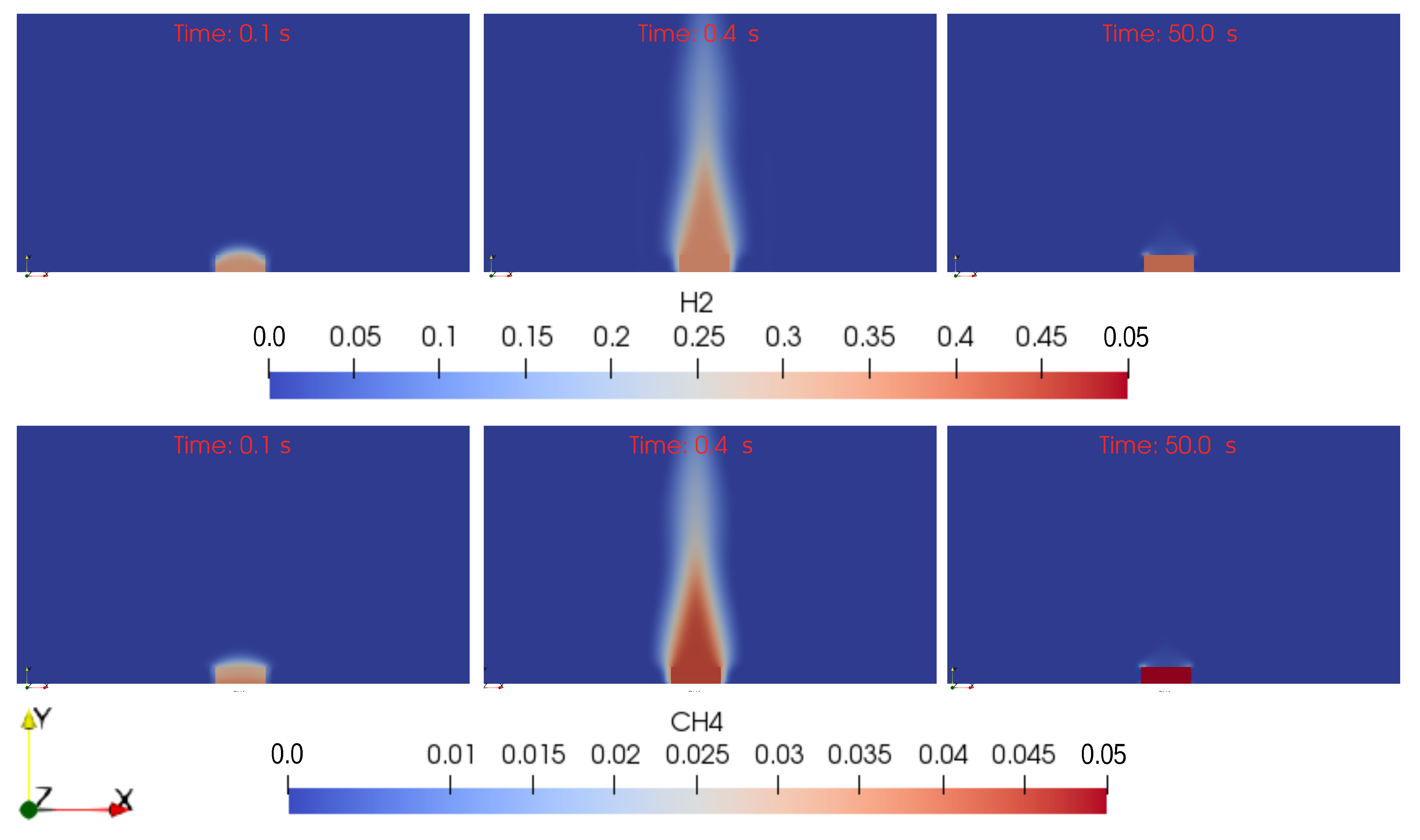
5.1. Hydrogen vs. Methane Flames

The first case considers the combustion of two gaseous species in the same domain. Two separate finite-rate combustion reactions have been considered

$${\mathrm{CH}}_4+2{\mathrm{O}}_2\to {\mathrm{CO}}_2+2{\mathrm{H}}_2\mathrm{O}$$

(30)

$$2{\mathrm{H}}_2+{\mathrm{O}}_2\to 2{\mathrm{H}}_2\mathrm{O}$$

(31)

The first reaction describe the combustion reaction for methane, CH${}_4$, where O${}_2$, CO${}_2$ and H${}_2$O indicate respectively the oxygen, carbon dioxide and the water. The second reaction is the combustion of hydrogen, H${}_2$. The kinetics of the two reactions has been modeled with an Arrhenius type formulation. The relative input parameters are showed in

Table 1. Kinetics parameters of the two combustion reactions. CH${}_4$ indicates the combustion of the methane, whereas H${}_2$ the combustion of the hydrogen.

	$\mathcal{A}$	$\mathit{\beta }$	${\mathit{T}}_{\mathit{a}}$
CH${}_4$	5.2 × 10${}^{16}$	0	14,906
H${}_2$	4.74 × 10${}^{12}$	0	10,064

.

The test case is schematized in Figure 4.

The domain corresponds entirely to the environment region. Air is considered as fluid. Air is initially composed of $21\%$ of O${}_2$ and $79\%$ of N${}_2$. At time $t=0$, methane and hydrogen are injected in the domain at two different positions at temperature 500 K. This temperature is high enough to trigger the two combustion reactions. Two flames propagate in the domain as shown in Figure 5.

Different time intervals are considered. For each of them the flames are colored based on the temperature. The two flames are different. The one on the left, that is the one due to the hydrogen combustion, is smaller and generates more energy than the one due to the combustion of methane. This is just a confirmation of what is known from the theory [30]. The hydrogen mixture burns faster than the one of methane and reaches higher temperatures (2500 K against 2100 K).

This simple case proves the importance of introducing different pyrolysis species in the overall problem. The flame, and so the overall simulation, strongly depends on the species taken into account.

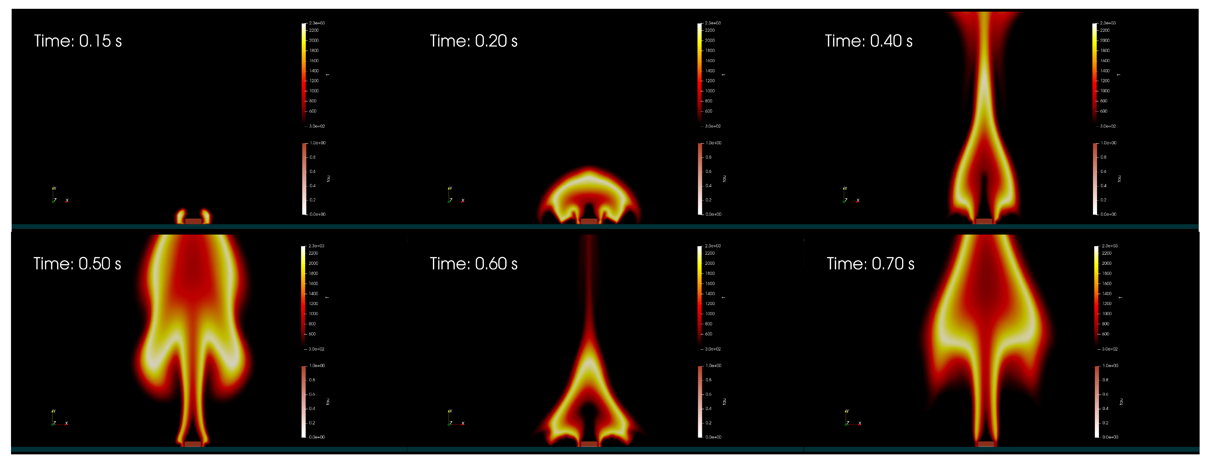
5.2. Wood Log Combustion

The second case aims to simulate the combustion of a wood log. The computational domain is schematized in Figure 6.

A wood log with a porosity ${ϵ}_w=0.5$ is placed at the bottom of the domain. It is modeled as being composed of 4 phases: hemicellulose, lignin, cellulose and water. The phases composition reflects a generic hardwood. Air, with the same composition as in the previous case, is surrounding it. At time $t=0$ the bottom part of the log is heated up by a Dirichlet condition at 800 K. Due to the heat, different pyrolysis reactions are triggered. A list of them with the considered kinetic parameters can be found in

Table 2. Pyrolysis reactions and kinetic parameters. The four species (hemicellulose, cellulose, lignin, and water) undergo different degradation processes according to the chemical reactions listed in this table.

j	Hemicellulose	${\mathit{F}}_{1,\mathit{j}}$	${\mathcal{A}}_{1,\mathit{j}}$	${\mathcal{E}}_{1,\mathit{j}}$	${\mathit{m}}_{1,\mathit{j}}$	${\mathit{n}}_{1,\mathit{j}}$
1	$p_{1,1}⟶0.4{\mathrm{H}}_2+0.4\mathrm{CO}+0.1{\mathrm{CO}}_2+0.05{\mathrm{CH}}_4+0.05{\mathrm{N}}_2$	0.40	7.94 × 10${}^{16}$	195,000	1	0
2	$p_{1,2}⟶0.4{\mathrm{H}}_2+0.4\mathrm{CO}+0.1{\mathrm{CO}}_2+0.05{\mathrm{CH}}_4+0.05{\mathrm{N}}_2$	0.30	1.26 × 10${}^7$	106,000	1	0
	Cellulose
1	$p_{2,1}⟶0.4{\mathrm{H}}_2+0.4\mathrm{CO}+0.1{\mathrm{CO}}_2+0.05{\mathrm{CH}}_4+0.05{\mathrm{N}}_2$	0.75	7.94 × 10${}^{18}$	202,650	1	0
2	$p_{2,2}⟶0.4{\mathrm{H}}_2+0.4\mathrm{CO}+0.1{\mathrm{CO}}_2+0.05{\mathrm{CH}}_4+0.05{\mathrm{N}}_2$	0.16	1.26 × 10${}^7$	245,000	1	0
	Lignin
1	$p_{3,1}⟶0.4{\mathrm{H}}_2+0.4\mathrm{CO}+0.1{\mathrm{CO}}_2+0.05{\mathrm{CH}}_4+0.05{\mathrm{N}}_2$	0.66	6.0 × 10${}^7$	120,000	1	0
	Water
1	$p_{4,1}⟶{\mathrm{H}}_2\mathrm{O}$	1	5.13 × 10${}^6$	86,000	1	0

.

All the phases undergo different pyrolysis reactions, each characterized by different parameters. The species, once produced, percolate through the material and eventually reach the external environment. At time $t=0.15$ s, two sparks are simulated at the two sides of the log. These sparks have the purpose of triggering the combustion. Methane and hydrogen start to burn and the fire evolves according to the concentration of the species in the air. Some snapshots of the first physical second of the simulation are collected in Figure 7.

At around 30 s of physical time, the wood log is completely pyrolyzed. At around 50 s of physical time, the fire is turned off due to the lack of fuel. Results in terms of H${}_2$ and CH${}_4$ concentration are showed in Figure 8.

In the figure it can be appreciated how the concentrations of the gaseous species change in time and depend on the pyrolysis activity in the material region. The latter is captured by the parameter $\tau$ (Equation (3)), that describes the advancement of the overall pyrolysis process. When $\tau =1$, no chemical reaction has yet occurred. When $\tau =0$ all the pyrolysis mechanisms have taken place and only char is left in the material. Some snapshots of the evolution of this parameter during the simulation are shown in Figure 9.

Four different time steps have been captured, and each of them focuses on the material region. It can be appreciated how the log evolves from the initial state to the final one, where only char is left. At around 30 s of physical time, all the pyrolysis reactions are completed and gas is no longer produced. Once the flame in the environment region has consumed all the fuels (CH${}_4$ and H${}_2$), the fire extinguishes.

A particular effect that is captured in this simulation is the so called “puffing phenomenon”. It is an instability effect of the fire due to gravity, which results in a pulsation behavior. These periodic fluctuations of the fire are repeated in time with a frequency f. In Figure 7 the effect can be observed by looking the time laps $t=0.5\mathrm{s}$ and $t=0.7$ s. The two snapshots both represent the end of the respective pulsation and they are quite similar. We can deduce that for the numerical simulation, the frequency of the puffing effect is about $f_{sim}\approx 5$ Hz. Different studies attempted to study this effect and to try to correlate it with physical dimensions [31,32,33]. A power law has been defined to fit the data

$$f_{pl}=1.5{\displaystyle \frac{1}{\sqrt{L}}}$$

(32)

where L in this case is the burner diameter. By considering the diameter of the fire at the base as the measure of L, it is possible to find out that this correlation gives us $f_{pl}\approx 7$ Hz. The two measures of the puffing frequency are approximately the same.

6. Conclusions

This study proposes a new numerical framework to investigate the combustion of pyrolysis materials. A detailed three-dimensional pyrolysis model is coupled with fireFoam, a numerical solver for combustion processes. The pyrolysis model captures the physics in the material region and describes the interaction between a multi-phase reactive material with a multi-species reactive gas mixture. The description is done at the macroscopic scale, where the governing equations are derived from upscaling theories. FireFoam is used to describe the environment region. Its governing equations are derived from the Navier-Stokes equations after applying the LES filtering process and using the Favre mean variables. The two models are coupled at the material-environment interface, where specific conditions for velocity, pressure, temperature and species concentration are imposed. Two applications are considered to illustrate the capabilities of the tool. The first one considers the combustion of two different gaseous species with the implementation of two separate finite-rate combustion reactions. Results show how the two generated flames differ between each other in terms of temperature and reaction times. The behavior of the flames is strongly influenced by the pyrolysis species considered in the model. The second case illustrates the combustion of a wood log. Results illustrate how gaseous species are produced with time through the pyrolysis of the wood log and how these species enter in the environmental region to start and sustain the flame. Thanks to the flame and to the temperature increase, the pyrolysis processes speed up and the species concentrations continuously change in time according to the rate of reactions. Once the wood is fully pyrolyzed, the fire consumes all the fuels and extinguishes by itself. The puffing effect can be observed during the evolution of the simulation: the fire exhibits periodic fluctuations that follow each other with a numerical frequency that is approximately the same as the theoretical one.

The numerical framework that was developed during this study is available in the Porous material Analysis Toolbox based on OpenFoam (PATO) released Open Source by NASA (www.pato.ac (accessed on 14 September 2021)) [34].

References

1. Östman, B.; Brandon, D.; Frantzich, H. Fire safety engineering in timber buildings. Fire Saf. J. 2017, 91, 11–20. [Google Scholar] [CrossRef] [Green Version]
2. Cox, G.; Moss, J. Fire science and aircraft safety. In Proceedings of the AGARD Conference Proceedings, The Hague, The Netherlands, 8–12 May 1989. [Google Scholar]
3. Mouritz, A.P.; Gibson, A.G. Fire Properties of Polymer Composite Materials; Springer Science & Business Media: Berlin/Heidelberg, Germany, 2007; Volume 143. [Google Scholar]
4. Dasari, A.; Yu, Z.Z.; Cai, G.P.; Mai, Y.W. Recent developments in the fire retardancy of polymeric materials. Prog. Polym. Sci. 2013, 38, 1357–1387. [Google Scholar] [CrossRef]
5. Delichatsios, M.; Paroz, B.; Bhargava, A. Flammability properties for charring materials. Fire Saf. J. 2003, 38, 219–228. [Google Scholar] [CrossRef]
6. Fateh, T.; Richard, F.; Batiot, B.; Rogaume, T.; Luche, J.; Zaida, J. Characterization of the burning behavior and gaseous emissions of pine needles in a cone calorimeter—FTIR apparatus. Fire Saf. J. 2016, 82, 91–100. [Google Scholar] [CrossRef]
7. White, R.H.; Dietenberger, M.A. Fire safety. In Wood Handbook: Wood as an Engineering Material; General Technical Report FPL; USDA Forest Service, Forest Products Laboratory: Madison, WI, USA, 1999; Volume 113, pp. 17.1–17.16. [Google Scholar]
8. Global, F. fireFoam. Available online: http://code.google.com/p/firefoam-dev/ (accessed on 14 September 2021).
9. Li, Y.Z.; Huang, C.; Anderson, J.; Svensson, R.; Ingason, H.; Husted, B.; Runefors, M.; Wahlqvist, J. Verification, Validation and Evaluation of fireFoam as a Tool for Performance Design. 2017. Available online: http://www.diva-portal.org/smash/record.jsf?pid=diva2%3A1166638 (accessed on 14 September 2021).
10. Zamorano, R. fireFoam (CFD Solver) Validation in Compartment Fire Scenario Using High Resolution Data. 2018. Available online: https://www.semanticscholar.org/paper/Firefoam-(CFD-solver)-validation-in-compartment-Zamorano/bd0ba6c49d5073adc6379008b56ec9182c1ec164 (accessed on 14 September 2021).
11. Trouvé, A.; Wang, Y. Large eddy simulation of compartment fires. Int. J. Comput. Fluid Dyn. 2010, 24, 449–466. [Google Scholar] [CrossRef]
12. Yang, H.; Yan, R.; Chen, H.; Lee, D.; Zheng, C. Characteristics of hemicellulose, cellulose and lignin pyrolysis. Fuel 2007, 86, 1781–1788. [Google Scholar] [CrossRef]
13. Blondeau, J.; Jeanmart, H. Biomass pyrolysis at high temperatures: Prediction of gaseous species yields from an anisotropic particle. Biomass Bioenergy 2012, 41, 107–121. [Google Scholar] [CrossRef]
14. Nunn, T.; Howard, J.; Longwell, J.; Peters, W. Product compositions and kinetics in the rapid pyrolysis of milled wood lignin. Ind. Eng. Chem. Process. Des. Dev. 1985, 24, 844–852. [Google Scholar] [CrossRef]
15. Di Blasi, C. Modeling chemical and physical processes of wood and biomass pyrolysis. Prog. Energy Combust. Sci. 2008, 34, 47–90. [Google Scholar] [CrossRef]
16. Chan, W.; Kelbon, M.; Krieger, B. Modelling and experimental verification of physical and chemical processes during pyrolysis of a large biomass particle. Fuel 1985, 64, 1505–1513. [Google Scholar] [CrossRef]
17. Miller, R.; Bellan, J. A generalized biomass pyrolysis model based on superimposed cellulose, hemicelluloseand liqnin kinetics. Combust. Sci. Technol. 1997, 126, 97–137. [Google Scholar] [CrossRef]
18. Ranzi, E.; Cuoci, A.; Faravelli, T.; Frassoldati, A.; Migliavacca, G.; Pierucci, S.; Sommariva, S. Chemical kinetics of biomass pyrolysis. Energy Fuels 2008, 22, 4292–4300. [Google Scholar] [CrossRef]
19. Lachaud, J.; Magin, T.; Cozmuta, I.; Mansour, N. A short review of ablative-material response models and simulation tools. In Proceedings of the 7th European Symposium on Aerothermodynamics, SP-692, European Space Agency, Noordwijk, The Netherlands, 9–12 May 2011; pp. 1–12. [Google Scholar]
20. Lachaud, J.; Mansour, N. Porous-material analysis toolbox based on OpenFOAM and applications. J. Thermophys. Heat Transf. 2014, 28, 191–202. [Google Scholar] [CrossRef]
21. Lachaud, J.; van Eekelen, T.; Scoggins, J.; Magin, T.; Mansour, N. Detailed chemical equilibrium model for porous ablative materials. Int. J. Heat Mass Transf. 2015, 90, 1034–1045. [Google Scholar] [CrossRef]
22. Lachaud, J.; Scoggins, J.; Magin, T.; Meyer, M.; Mansour, N. A generic local thermal equilibrium model for porous reactive materials submitted to high temperatures. Int. J. Heat Mass Transf. 2017, 108, 1406–1417. [Google Scholar] [CrossRef]
23. Favre, A. Turbulence: Space-time statistical properties and behavior in supersonic flows. Phys. Fluids 1983, 26, 2851–2863. [Google Scholar] [CrossRef]
24. Ferziger, J.H.; Perić, M.; Street, R.L. Computational Methods for Fluid Dynamics; Springer: Berlin/Heidelberg, Germany, 2002; Volume 3. [Google Scholar]
25. Erlebacher, G.; Hussaini, M.Y.; Speziale, C.G.; Zang, T.A. Toward the large-eddy simulation of compressible turbulent flows. J. Fluid Mech. 1992, 238, 155–185. [Google Scholar] [CrossRef] [Green Version]
26. Chase, M. NIST-JANAF Thermochemical Tables. 1998. Available online: https://janaf.nist.gov/ (accessed on 14 September 2021).
27. Shen, V.K.; Siderius, D.W.; Krekelberg, W.P.; Hatch, H.W. NIST Standard Reference Simulation Website-SRD 173. NIST Standard Reference Database Number 173; National Institute of Standards and Technology: Gaithersburg, MD, USA, 2017. [CrossRef]
28. Poling, B.E.; Prausnitz, J.M.; O’connell, J.P. Properties of Gases and Liquids; McGraw-Hill Education: New York City, NY, USA, 2001. [Google Scholar]
29. Xiao, H.; Jenny, P. A consistent dual-mesh framework for hybrid LES/RANS modeling. J. Comput. Phys. 2012, 231, 1848–1865. [Google Scholar] [CrossRef]
30. Sierens, R.; Demuynck, J.; Paepe, M.D.; Verhelst, S. Heat Transfer Comparison between Methane and Hydrogen in a Spark Ignited Engine. 2010. Available online: https://juser.fz-juelich.de/record/135724/files/TA3_3_Sierens.pdf (accessed on 14 September 2021).
31. Mandin, P.; Most, J. Characterization of the puffing phenomenon on a pool fire. Fire Saf. Sci. 2000, 6, 1137–1148. [Google Scholar] [CrossRef] [Green Version]
32. Beyler, C.L. Fire plumes and ceiling jets. Fire Saf. J. 1986, 11, 53–75. [Google Scholar] [CrossRef]
33. Pretrel, H.; Audouin, L. Periodic puffing instabilities of buoyant large-scale pool fires in a confined compartment. J. Fire Sci. 2013, 31, 197–210. [Google Scholar] [CrossRef]
34. Lachaud, J.; Meurisse, J. Porous Material Analysis Toolbox Based on OpenFOAM. Available online: http://pato.ac/ (accessed on 14 September 2021).
Figure 1. A generic combustion problem. Two different regions are present: the environment, where combustion happens, and the material, characterized by pyrolysis.
Applsci 11 10570 g001
Figure 2. Illustration of the problem: interaction between a multi-phase reactive material with a multi-species reactive gas mixture. The model characterizes this problem at the macroscopic scale under the assumption of scale separation ( L > > l ).
Applsci 11 10570 g002
Figure 3. Illustration of the numerical boundary conditions for the coupling between the two regions. Conditions for the velocity, temperature, pressure and species concentration need to be imposed.
Applsci 11 10570 g003
Figure 4. Illustration of the test case: methane and hydrogen are introduced, at initial time, at high temperature inside a domain of air. The combustion reactions for both species are implemented.
Applsci 11 10570 g004
Figure 5. Temperature description in the domain. Three different time steps are considered. The figures show on the left the flame generated by the hydrogen combustion and on the right the one generated by the methane combustion. The two flames are different from each other. They differ both in terms of temperature and in terms of size.
Applsci 11 10570 g005
Figure 6. Numerical domain for the simulation of the burning of a wood log. A generic hardwood composition has been considered for the log. Air, with simplified composition, has been taken as flow.
Applsci 11 10570 g006
Figure 7. Starting of the fire. Six different snapshots to represent the initial evolution of the fire. At time t = 0.15 s two sparks are generated on the side of the wood log to trigger the combustion. A fire is generated and start propagating in the domain. By comparing the time t = 0.50 s with the time t = 0.70 s it is possible to observe the periodic behavior of the flame, the puffing effect.
Applsci 11 10570 g007
Figure 8. Concentration of hydrogen and methane in the simulation. It can be observed how their concentration is time dependent. At time t = 0.1 s the concentration of the gases in the environment region is close to zero. With time, thanks to the advancement of pyrolysis, their concentration increases. For the two gases different values of concentration are reached. At time t = 50 s it can be see that the fire has consumed the two species and their concentration is again nearly zero.
Applsci 11 10570 g008
Figure 9. Advancement of pyrolysis of the wood log during the simulation. When τ = 1 , no chemical reactions has still occurred. When τ = 0 all the pyrolysis mechanisms have taken place and only char is left in the material. At time t = 0.5 s it can be seen how the pyrolysis process starts from the bottom of the material and at time t = 30 s how all the material has been pyrolysed.
Applsci 11 10570 g009