Featured Application
The e-behaviour, personality and performance evaluation frameworks described in this article can be used by students and academic staff alike to monitor performance and online behaviour as it relates to performance. Being aware of e-behavioural patterns is a starting point to improving the academic performance of individual students and groups of students. The methodology can be used to inform the extent to which a course is to be adapted such that it encourages students to engage in behaviour that promotes better academic performance.
Abstract
The analysis of student performance involves data modelling that enables the formulation of hypotheses and insights about student behaviour and personality. We extract online behaviours as proxies to Extraversion and Conscientiousness, which have been proven to correlate with academic performance. The proxies of personalities we obtain yield significant () population correlation coefficients for traits against grade— for Extraversion and for Conscientiousness. Furthermore, we demonstrate that a student’s e-behaviour and personality can be used with deep learning (LSTM) to predict and forecast whether a student is at risk of failing the year. Machine learning procedures followed in this report provide a methodology to timeously identify students who are likely to become at risk of poor academic performance. Using engineered online behaviour and personality features, we obtain a Cohen’s Kappa Coefficient () of students at risk of . Lastly, we show that we can design an intervention process using machine learning that supplements the existing performance analysis and intervention methods. The methodology presented in this article provides metrics that measure the factors that affect student performance and complement the existing performance evaluation and intervention systems in education.
1. Introduction
The evaluation and analysis of the factors that affect the academic performance of tertiary students stem from a need to improve student throughputs. Richiţeanu-Năstase and Stăiculescu [1] identify several reasons why post-secondary educational institutions have a low rate of completion. They name three main reasons: first, a lack of support (such as academic counselling services), second, the student’s background, and third, an inability to adapt to the curriculum.
In addressing student performance, we consider their grades at the end of a study programme as a measure of their performance. We also refer to performance as risk or risk of failure since an increase in performance results in a lowered risk of failure. The e-behaviour of a student is “a pattern of engagement with a Learning Management System (LMS)”, and personality according to Wright and Taylor [2] refers to “[…] the relatively stable and enduring aspects of individuals which distinguish them from other people and form the basis of our predictions concerning their future behaviour”.
Traditional approaches to revealing relationships between student behaviour, personality and performance include questionnaires, surveys and interviews. The reliability of a questionnaire would depend on the contextual framework for the research and the metric construct used for outcomes. However, respondents’ biases from the above qualitative methods of data collection can compromise the accuracy of their responses [3,4,5]. Furthermore, it has not proven easy to measure the reliability of an opinion [6], especially for each individual in a population. We address the self-reporting problems using unobtrusive and automated approaches that measure how students behave rather than how they think they behave. For instance, instead of asking, ‘In how many weekly online discussions do you participate?’, we instead obtain the exact number of discussions from an LMS register. The models developed in this research use quantitative metrics to proxy behaviour and personality traits traditionally obtainable from surveys. These metrics are used to draw correlations with features later used to predict student performance. From e-behaviour and personality, we modelled an intervention framework that supplements current student intervention systems.
We extract behavioural insights linked to two of the five personality traits in the Big Five personality model through a quantitative analysis—Conscientiousness and Extraversion. We use statistical metrics to extract forum and login behaviours, respectively. We define the relationships between these metrics and online behaviours, detailing the relationships between a student’s expressions of personality traits through their behaviours. Through this research, we:
- Define a framework for personality traits and behaviour in the context of student online engagement;
- Show the relationship between Bourdieu’s Three Forms of Capital and academic performance;
- Show the relationship between personalities and academic performance through e-behaviours;
- Show that we can use e-behaviour and machine learning to predict student performance;
- Highlight the importance of the explainability of modelled personality traits and e-behaviours.
This work contributes to the prediction of student outcomes using online behaviours in the following ways:
- We present a framework and methodology for arriving at predictive models for student performance starting with personality traits. These traits are the drivers of online behaviours that generate features that are predictive of performance.
- We argue for the use of online behaviours and proxies for the personality traits Conscientiousness and Extraversion.
- We demonstrate that online behaviours that are strongly associated with the identified personality traits correlate with student performance in a statistically significant way.
1.1. Literature Review
A standard psychological framework for measuring personality is the Five-Factor or OCEAN (Openness, Conscientiousness, Extraversion, Agreeableness and Neuroticism) model (Costa and McCrae [7], Poropat [8], Furnham et al. [9], Ciorbea and Pasarica [10], Kumari [11], Morris and Fritz [12]). Recent research by Morris and Fritz [12] has shown that Conscientiousness and Extraversion are significantly correlated with student educational outcomes. In this research, we build upon the vast body of literature that supports these two personality traits as being correlated with student performance [8,9,10,11,12,13,14].
A revised Neuroticism–Extraversion–Openness Personality Inventory (NEO PI-R) [15] expands each of the OCEAN personality trait’s six facets. For Conscientiousness, these facets are competence, orderliness, dutifulness, achievement striving, self-discipline and deliberation. Activity, assertiveness, excitement seeking, gregariousness, positive emotion and warmth are the facets of Extraversion. Wilt and Revelle [16] define Extraversion as the ‘disposition to engage in social behaviour’, which links significantly to the gregariousness facet. Gregariousness is defined as the ‘tendency for human beings to enjoy the company of others and to want to associate with them in social activities’ [17]. Dutifulness is defined as the characteristic of being motivated by a sense of duty [18]. In this article, we model for the orderliness facet of Conscientiousness and the gregariousness facet of Extraversion.
Recent work by Akçapınar [19] and Huang et al. [20] has shown that the usage of online behaviours alone does not necessarily lead to features that are predictive of student performance. We argue that this may be due to the many features that can be engineered from the time series of log data representing online student behaviour. For instance, the Tsfresh library can extract over 40 time-series features. The link between online behaviours and the personalities that underlie them has not been extensively explored. We follow the argument of Khan et al. [21] and postulate that starting from a principled approach that is grounded in personality traits will lead to a more viable set of features and metrics.
Contribution to Existing Evaluation Systems
The University of Witwatersrand’s (the University’s) academic and student support staff members have access to three standard systems of identifying the likelihood of students completing a programme. These systems can be broadly grouped into grades, questionnaires, observing a student’s grades for that programme over time, and one-on-one consultations by a counsellor or lecturer with the student.
Questionnaires have two significant limitations. Firstly, they are not offered throughout the teaching period and, secondly, they are anonymous, meaning there is no easy way of linking students at risk to their programmes. Fowler and Glorfeld [22], Poh and Smythe [23], Evans and Simkin [24] show that prior performance or grades are a reliable measure for future performance. By their high-touch nature, observing grades and consultations are usually not anonymous. The advantage of these two systems is that they give a detailed response to students’ feelings towards their programmes and are, thus, potentially corrective (can help resolve poor performance). The disadvantages are that one-to-one consultations and grades are often retroactive rather than proactive and not conducted at scale or sufficiently continuously.
The limitations in gauging student performance through the above mechanisms give rise to a proposal for using e-behaviour machine learning models, while models that fit students’ e-behaviour do not guarantee similar reliability, e-behaviour machine learning models have some advantages over grades, questionnaires and consultations. Table 1 shows a comparison of evaluation systems. Whether an evaluation system is continuously proactive, corrective, feasible at scale and reliable depends on:

Table 1.
Comparison of evaluation systems.
- The contextual framework for the research;
- The metric construct used for measuring each of these variables and outcomes;
- How the variables are used in an academic setting.
In Table 1, note that e-behaviour models are the only system of evaluation that is continuously proactive—can be monitored at any point in time to take corrective action.
1.2. Bourdieu’s Three Forms of Capital and Student Success
Bourdieu’s Three Forms of Capital is a framework that suggests that economic, cultural and social capital that an individual can leverage regulates their level of success. We use this framework to support our investigation of the economic, cultural and social capital that a student has available to them as each form of capital relates to their academic performance. Dauter [25] defines economic sociology as
“[…] the application of sociological concepts and methods to the analysis of the production, distribution, exchange, and consumption of goods and services.”
Economic sociology has been used extensively by Bourdieu and Richardson [26], who argue that an individual’s possession of three forms of capital regulates their social positions and ability to access goods and services. These three forms of capital are economic capital, cultural capital and social capital. The Three Forms can be considered essential to a student obtaining good grades and acquiring the services they need to improve their grades. We refer to our proxies for economic and cultural capital as the background of a student.
1.2.1. Social Capital
Bourdieu and Richardson [26] define social capital as:
“The aggregate of the actual or potential resources which are linked to the possession of a durable network of more or less institutionalised relationships of mutual acquaintance and recognition.”
The above definition describes social capital as a resource that is available between people due to their relationships. An individual may accrue social capital by being part of relationships. Carpiano [27] uses the framework by Bourdieu and Richardson [26] to build onto the theory of social capital. Carpiano [27] categorises the social capital available to individuals into four types, namely: social support, social leverage, informal social control and community organisation participation.
The above four types of social capital are available to students, forming relationships for social or academic purposes. Hallinan and Smith [28] refer to these intra-cohort groups as social networks or cliques. The common saying, show me your friends and I will show you your future, is commonly used to describe the relationship between an individual’s affiliates and their results. In this research, these results are referred to as their Grade or their Outcome. The hypothesis that a student has access to some social capital has been validated to various extents by Hallinan and Smith [28] and is also adopted in this research.
A limitation with the social capital frameworks by Bourdieu and Richardson [26], Carpiano [27] and Song [29] is that they provide no standard measure of social capital. The definition of social capital leaves no room for a well-defined metric. In our research, a student’s social network is evidence of their social capital and is called their Academic group. In an academic setting, a student’s quality of resources social capital can be defined in terms of the aggregate grades of their Academic group. The relationships between Academic groups and Grades is modelled in Section 3.4 and Section 3.5.
1.2.2. Cultural Capital
According to Hayes [30], cultural capital is a set of non-economic factors that influence academic success, such as family background, social class and commitments to education, and do not include social capital. Bourdieu and Richardson [26] categorise cultural capital into three forms, namely:
- Institutionalised cultural capital (highest degree of education);
- Embodied cultural capital (values, skills, knowledge and tastes);
- Objectified cultural capital (possession of cultural goods).
In this research, the features we selected in Section 2.5 are proxies of 1 and 2. Smith and White [31] found that success in obtaining a degree relates strongly to gender and ethnicity. Caldas and Bankston [32] found that students’ cultural capital affects their performance.
1.2.3. Economic Capital
Bourdieu and Richardson [26] define economic capital as material assets that are ‘immediately and directly convertible into money’. In turn, an individual’s monetary leverage can be converted into cultural and social capital [26].
Bourdieu and Richardson [26] recognise that an individual can increase their social and cultural capital by making use of their economic capital. An individual who leverages their economic capital can obtain more resources to improve their cultural capital. For instance, an individual can improve their cultural capital through improvement in their position in society. By investing in formal or informal education beyond the classroom, a student may increase their knowledge and the amount of cultural capital available to them. Fan [33] observed that a student’s quality and level of education was affected by their cultural and economic capital.
Section 3.1 reveals the relationships between student background (background refers to cultural and economic capital) and academic performance.
2. Methodology
2.1. Data Preprocessing
The data were composed of files with logs on the Moodle LMS database at our university for first-, second-and third-year students who were enrolled in Applied Mathematics and Computer Science modules in the 2018 academic year. After examining distributions and removing students who had no grade records, the data were reduced to time series patterns, aggregated by each day of the semester. The models were fitted on the open-semester logs recorded (from the beginning of the semester till two weeks before exams). The advantage of using only open-semester data was not only that it helped us understand the predictive power of the behaviour, but it also eliminated effects of sudden changes in behaviours that were forced upon students as examinations approached [12]. The target variable for all experiments was the aggregate Grade (out of 100 points) of online assessments, including examinations, that the student obtained over the year.
2.2. Importance and Choice of Personality Traits
The university LMS contained several tables that each provided different information. We checked each table’s appropriateness in modelling any of the OCEAN traits. The Forums and Logins Tables contained logs with details about student interaction, and were, thus, chosen as primary tables from which to source behavioural information for our proxies for Conscientiousness and Extraversion. By comparison, Openness, Agreeableness and Neuroticism were more complex to model, given the available data and the lack of validation of a link to academic performance within the literature.
Our data linked closest to the dutifulness facet of Conscientiousness and the gregariousness facet of Extraversion. Alternative formulations of each trait were considered and are described in Section 5.1. We used quantitative proxies to model Conscientiousness (Dutifulness) and Extraversion (Gregariousness).
2.3. Encoding Personality Traits
According to Ajzen [34], Campbell [35], human behaviour can be explained by reference to stable underlying dispositions or personality. Wright and Taylor [2] define personality as:
‘the relatively stable and enduring aspects of individuals which distinguish them from other people and form the basis of our predictions concerning their future behaviour’.
Therefore, Extraversion and Conscientiousness were modelled as single-valued averages that did not vary through time. Our choice to encode personality traits as unvarying values was based on the theory by Wright and Taylor [2], Ajzen [34], Campbell [35], Hemakumara and Ruslan [36].
We acknowledge that ‘there is a complex relationship between personality and academic performance’ [8]. As a result, the same complexities could be expected between our proxies of Conscientiousness, Extraversion and Performance. These relationships were not controlled for, since they were not present in our data. However, given the data and interaction between them, it was important to control for the variables, in light of research by Poropat [8].
Challenges against Encoding Personality Traits
The above definitions of personality and their link to behaviour may cause a belief that personality and behaviour should be measured identically. However, to understand the separate correlations between either personality and performance or e-behaviour and performance, it was essential to encode an individual’s stable aspects (personality traits that are less likely to change) differently from their changing e-behaviour. As a result, personality metrics were aggregated while e-behaviour was modelled to vary over time.
2.4. Encoding Performance
Three measures of performance were constructed, namely, Grade, Outcome and derived Safety Score. Grade is a continuous label that indicates the mean of a student’s performance across all modules taken. This label was continuous and ranged between 0.00 and 100.00. Outcome is a binary label that indicates whether a student obtained below 51 Grade points (At-risk) or at least 51 Grade points (Safe). That is, the Outcome was taken to measure the degree of risk-of-failure. Note that a fail was considered any grade below 50 Grade points. However, the boundary of 51 provided a buffer that allowed the models to reveal students who were close to failing (At-risk). Therefore, a student need not fail for them to be considered at risk. A student’s Safety Score is a classification label used as a label of their predicted Outcome. A correct classification would assign a Flagged Safety Score for an At-risk student and an Ignored Safety Score for a student with a Safe Outcome.
Grade was used as a regressor against Extraversion level (Section 2.6) and Conscientiousness level (Section 2.9). Outcome was used as a label to the classification models in Section 2.5 and Section 2.10.
2.5. Student Background
The raw Background Dataset consisted of 4748 students and 176 features on which experiments were conducted. These features captured answers by the student upon registration and data collected throughout their study—for instance, their high-school facilities, high-school subjects, age and city of residence. Table 2 shows a summary of the features after each phase of transformation.
Table 2.
Background data feature count per phase of transformation.
The 169 categorical features were one-hot encoded, extending the number of features from 176 to 6623. Recursive Feature Elimination algorithm (RFE) with a Decision Tree was used to reduce the 6623 feature set’s dimensionality.
Feature Selection Using RFE
RFE involved filtering through features with the lowest ranking of importance against Outcome, through the following procedure [37]:
- Optimise the Decision Tree weights with respect to their objective function on a set of features, F;
- Compute the ranking of importance for the features in F using the Decision Tree optimiser;
- Prune the features with the lowest rankings from F;
- Repeat 1–3 on the pruned set until the specified number of features is reached.
The RFE process produced five Background Features, explained with the Grade and Outcome variables in Table 3.
Table 3.
Background data features and labels after RFE.
2.6. Extraversion and Academic Groups
Discussion, Message and Time independent variables, explained in Table 4, were used to engineer the Extraversion level (Extraversion level was the proxy for Extraversion) of a student, as well as formulate the Discussions and Collaboration groups.
Table 4.
Forum table features.
Forum Posts and Extraversion
The definition of social capital in Section 1.2 suggests that Extraversion or gregariousness can improve an individual’s ability to accumulate social capital, which is correlated with academic performance. A way to model social interaction or gregariousness is by capturing the number of forum posts that an individual contributes to forum discussions. Hence, we chose the student’s post count as a quantitative proxy for their level of Extraversion.
Each student was placed in an Extraversion-level group, E, representing the number of posts they contributed. Each level, E, was then assigned a mean Grade, , computed by averaging the grades of all students in E. Table 5 shows the each Extraversion-level above its associated Grade.
Table 5.
Input table–Extraversion level Grade against Extraversion level.
2.7. Student Discussions
A Discussion (group), , was defined as any discussion that contains more than two students created on the Moodle LMS. A Discussion that had fewer than three students was not considered a Discussion by our definition. Linear OLS assumptions for Discussions containing only two or more students did not hold. Section 4.4 shows the reasons. Let D = be the set of all Discussions, represent any student who participated in discussion , represent a selected random student who participated in discussion , represent the mean Grade of Discussion and is the grade of student .
where k represents the number of Discussions in D and denotes the number of students in . This section measured the correlation between and by following Algorithm 1:
| Algorithm 1: Correlation Between Mean Discussion Grade and Student Grade. |
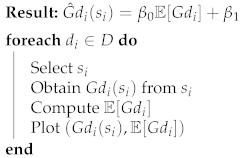 |
Table 6 shows a sample of random student Grades against their Discussion’s Grade Averages.
Table 6.
Discussion table—random student’s Grades against Discussion’s Grade averages.
2.8. Student Collaboration Groups
This section illustrates an alternative method to formulating an Academic Group, namely, the Collaboration group method. We correlated the Grades of students within each Collaboration group with the mean Grade of each Collaboration group.
The raw Forum Table was transformed into Table 7 below, which shows discussion participation per student. Each column, , represents a discussion: 1 represents that the student participated in discussion , while 0 shows that they did not participate in .
Table 7.
Sample table of Discussion participation.
Let C = be the set of all Collaboration groups. is the Host of with H = being the set of all Hosts, one for each Collaboration group.
A Collaboration group, , that was hosted by student, , was defined as the group of more than two students with whom shared at least one discussion. Any group with two or fewer students was not considered a Collaboration group by our definition; OLS relationships analogous to those in this section did not hold for groups containing only two or more students. The reasons were presented under Section 4.4. may host a maximum of one Collaboration group. Let represent a the mean Grade of , and represent the Grade of where represents the mean Grade of which excludes , as in the case with and in Equation (1).
The kNN algorithm was used to compute the Collaboration group for each student, using the Collaboration group policy specified in the below paragraph. By this policy, not all students fit the qualify to host a Collaboration group.
We designed the conditions necessary to define the Collaboration group policy; let be a candidate Host of a Collaboration group, with representing the Collaboration group to be hosted by student, . represents the number of students in , , and are any three students in the cohort, and represents a (qualified) Host to their (unique) Collaboration group, .
Collaboration group Policy: becomes a Collaboration group, , if and only if students. Equivalently, if shares a discussion with , and , then qualifies as a Host, , and . If students, then remains a candidate until they share a discussion with at least one more member.
A sample set of the Hosts, , and their Collaboration groups, is shown in Table 8. Each entry in column was a set of indices that represented students in , while column showed the Grades of the Hosts. represented the mean Grades of each .
Table 8.
Collaboration—groups and grades.
2.9. Logins and Conscientiousness
Section 2.2 explained the facets that describe each personality trait. Our model of Conscientiousness related closely with dutifulness. Barrick et al. [38] and Campbell [39] theorise that Conscientiousness is linked to an individual’s choice to expend a level of effort. Therefore, modelling dutifulness required a formulation that captured the average logins per week that the student performed throughout the programme. This model of the Conscientiousness level captured the facet of dutifulness and the choice to expend effort (Conscientiousness level is the proxy for Conscientiousness). Let be a variable that represents the Conscientiousness level of student s. was modelled as the average number of logins over the period spanning a student’s active weeks. For each student, was formulated as:
where is the number of weeks spanned between the student’s first and last login.
The reason for modelling as the average number of active days per week instead of the total number of logins over the period was that the average normalised the data. Averaging reduced biases caused by differences in the number of days per cohort, per subject and programme, that students were expected to log in.
Each personality trait proxy was regressed against the students’ grades for the semester using the Ordinary Least Squares (OLS) regression method [40]. The associated slope and correlation coefficients, p-values and Slope coefficient with 95% confidence intervals were reported.
To date, several longitudinal studies investigating academic performance and personality have used effects, determines or predicts to mean the relationship or correlation between personality traits and performance (for example, works by Poropat [8], Chamorro-Premuzic and Furnham [13], Blumberg and Pringle [41] and Morris and Fritz [12]. Without knowing the causality of personality traits on performance in our study, we adopted the same terminology for ease of reference and comparison.
2.10. Behaviour–Personality and Behaviour Model
The Behaviour–Personality model (B-PM) consisted of two components: the behavioural component was the Login Sequences of students, while the personality component augmented the Login Sequences. The traits that composed the personality component were the Extraversion and Conscientiousness levels. The Behaviour Model (BM) consisted of only the Login Sequences of students as input.
For each student s, we engineered the Login Sequence (), Extraversion level () and Conscientiousness level ( by augmenting and as sequences of the same values that ran parallel to through time t. This augmentation formed a input array of sequences:
where is a sequence of values that vary through time t, is a sequence of the same value through time t, so that , and is a sequence of the same value through time t, so that for all Whole Numbers . (See Table 9.)
Table 9.
B-PM training input and output summary.
This method of augmenting inputs in parallel was guided by its usage in Leontjeva and Kuzovkin [42]. As a result, The B-PM input for each student was the array of sequences:
The B-PM output for each student was a Safety Score: Flagged for At-risk students, and Ignored for Safe students. These per student B-PM input and output structures are summarised in Table 9.
2.11. Algorithms for E-Behaviour, Personality and Performance Analysis
2.11.1. Decision Tree Classifier
The Decision Tree Classifier (DTC) is a supervised learning algorithm that iteratively assesses conditions on the values of features in a dataset to perform classification. DTC breaks down a decision-making process into a collection of simpler decisions, providing classifications that are easier to interpret than other statistical and machine learning models [43].
DTC Architecture
DTC was assembled from a root node, edges, internal nodes and leaf nodes. At the root node, DTC conducted a test on each observation’s value. Based on its value, the root node assigned a resolution represented by an edge, which the observation then traversed. At the end of the traversed edge was an internal node. An example of a node’s test was ‘Gender?’, and an example of an edge was ‘Female’. This decision process continued through the rest of the internal nodes until the tree reached a leaf node, where a classification was determined. See Mitchell [44] for details on the DTC architecture.
Gini Impurity Index—Decision Factors
During prediction, an observation was predicted as part of a class after being checked through a series of conditions. An optimal decision tree resulted in an optimal split. An optimal split was achieved when each leaf node had the fewest possible train-set misclassifications (lowest impurity), and the tree had not been overfitted. Entropy and Gini Impurity Index are two commonly used metrics for impurity. The Gini Impurity Index (Gini) measures the relative frequency that a randomly chosen element from that set would be mislabelled. A Gini score greater than zero describes a node that contains samples belonging to different classes. Raileanu and Stoffel [45] suggest that the difference between Entropy and Gini is trivial. This research used Gini, which was interpretable.
Gini Calculation
The Gini value decreased as a traversal was determined down the tree towards its leaf nodes. The decrease happened as each internal node’s condition aimed to separate the classes according to a criterion that resulted in more homogeneous separations and higher accuracy in the training data. However, as with other predictive models, a high training-set accuracy was generated at the risk of overfitting. A larger tree (with more edges and branches) was more likely to overfit than a smaller tree and could result in a Gini of 0 at the tree’s leaf nodes. A Gini of 0 represented the minimum probability of misclassification over the training set, but could result in weak generalisability over the test set. Therefore, smaller trees were preferred to larger trees [44].
The Gini impurity index was calculated using the formula:
where is the probability of class i.
Khalaf et al. [46] model DTCs on survey questions and answers that cover health, social activity and relationships of students to predict their academic performance. Topîrceanu and Grosseck [47] and Kolo et al. [48] provide literature in educational data mining and advocate for the use of the DTC due to its low complexity (with a run time of and high interpretability. In Section 3.1, the DTC was used to select student economic and social capital features and predict the student Outcomes.
2.11.2. Ordinary Least Squares Linear Regression Analysis
Ordinary Least Squares (OLS) Linear Regression is a statistical model that estimates the linear relationship between one or more independent variables (regressors) and a dependent variable (regressand) [49]. Throughout this research, only one independent variable was used per regression model. Using one independent variable per model isolated the effect of each variable on Grade. A Regression model with one independent variable was called a Simple OLS Regression model. Each estimated or predicted value, , derived from the line of best-fit shown in Equation (5), could be determined by:
where is the predicted value of the independent variable, . is the estimated slope coefficient of the model, representing the average marginal change in for a unit increase in . , the fitted intercept of the model, represents the expected value of when . is the residual term.
Every observed value, , had an associated estimate or prediction value, . The line of best-fit,
was obtained by minimising the sum of the squares in the difference between the observed and predicted values of the dependent variable,
The (linear) correlation coefficient between x and y was represented by r or . measured the extent to which the independent variable, x, was correlated with the dependent variable, y. That is, measured the degree of closeness of all points, , to the line of best-fit, . The correlation coefficient laid between −1 and 1, where a r of 1 or −1 meant that the change in y was directly proportional to the increase in x. In that case, x and y were stated to be perfectly correlated. That is,
for all values of i where and were defined, and where . r was computed by:
where represents the mean average of independent variable x and represents the mean average of dependent variable, y.
The p associated with showed the probability of a hypothetical value, , having an absolute value, , that was at least as high as the observed by chance. The level of significance, , was used as a threshold for a permissible p. In the domain relating to e-behaviour, personality and performance, the common used was 0.05, or a 5% level of significance. In our regression models, was accompanied by a ( = 95%) confidence interval, . Suppose p < for . This meant that from 100 experiments on similar sample distributions, fewer than 5 experiments would produce a value that laid outside of . Such a result meant that the regressor and regressand had a statistically significant correlation different from zero [49]. Statistical insignificance could indicate that x on its own did not yield reliable estimates, .
Statistical significance was important in analysing a student cohort’s behaviour, since statistical significance confirmed the existence of a statistical relationship. Empirical significance refers to the magnitude of [49] and was also a measure of the model’s practical value. One could be more confident in practical decisions if the relationship was not generated by chance (if the relationship was statistically significant). This chance was measured by the p.
2.11.3. Validity of OLS Regression Models
The data given in a model had to satisfy five OLS regression assumptions [49], namely:
- Normality of model residuals. The residual for each point was given by . was computed for the residuals, where s is the z-score returned by the test for skewness and k is the z-score returned by the test for kurtosis.
- Residual Independence or lack of Autocorrelation in Residuals.
- Linearity in Parameters.
- Homoscedasticity of Residuals.
- Zero Conditional Mean.
- No Multicollinearity in Independent Variables.
A linear relationship that violated the OLS assumptions was not fit for an OLS model. Therefore, we constructed only OLS relationships that satisfied the assumptions. Mentioned were experiments where the OLS assumptions were violated. Linearity in Parameters, Homoscedasticity of Residuals and Zero Conditional Mean were verified for all Regression experiments whose results were analysed. The No Multicollinearity assumption was not verified since all OLS regression experiments were Simple. See Gujarati and Porter [49] for further details on the formulation of the OLS Regression model.
2.12. Long Short-Term Memory
The Long Short-Term Memory algorithm (LSTM) is a deep-learning architecture designed to model sequences for prediction [50]. The LSTM has been used in studies that range from predicting weather-induced background radiation fluctuation by Liu and Sullivan [50], to human motion classification and recognition by Wang et al. [51].
The backpropagation through time algorithm computes the error, , at every time step, t, and, then, computes the total error. The LSTM’s parameters were updated to minimise the total error with respect to a weight parameter :
Letting represent the output at time t, represents the hidden state at time t and by applying the chain rule to the Recurrent Neural Network model, the total error in Equation (9) became:
where involves a product of Jacobian matrices:
Equation (11) illustrates the problem of vanishing gradients in Equation (9): when the gradient became progressively smaller as k increased, the parameter updates became insignificant.
LSTMs are an architecture of Recurrent Neural Networks (RNNs). Bengio et al. [52] suggest that RNNs are challenging to train because of the vanishing error gradient problem. The following section stipulates how the LSTM’s architecture mitigates the vanishing error gradient issue through LSTM cells that maintain a state at every iteration t. The cell state serves to remember and propagate cell outputs between time steps. Each cell state then allows for temporal information to become available in the next time step, adding greater context to the inputs that follow.
The activation of an LSTM unit was:
where
is an output gate that mitigates the amount of content in the memory to expose to the following time step and is the logistic sigmoid function.
Given new memory content,
where represents the degree to which new memory is added to the memory cell, and is specified by an input gate
the cell state,
could be updated by taking into account the previous cell state and a term defined by the forget gate,
Consolidating Equations (12) to (17), the system of equations that describe each LSTM unit given by:
Let B denote the input batch size (number of time stamps per input chunk), H denote the LSTM hidden state capacity, and D represent the dimensions of the inputs to the LSTM. Then, in Equations (18) through (23):
For an illustration, refer to Figure 1. The LSTM had four main gates that responded to the values of four functions determined by and , represented in Equations (18) through (21). With the input data matrix (data vector if B = 1) concatenated with previous output matrix (vector if B = 1), the flow of inputs and outputs from the various gates described in the LSTM equations interacted as follows:
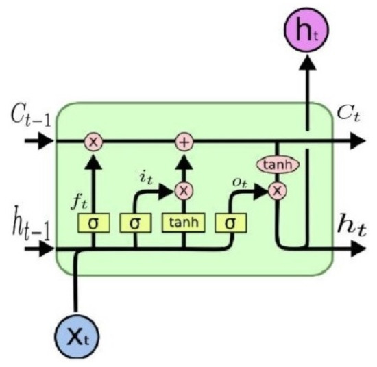
Figure 1.
The LSTM unit kept a cell state throughout its operations, which served as input in the next time step. It also output , which supplemented the input in the following time step. From Olah [53].
- and were fed into the gate (or function) , where the output laid in the open interval . then interacted with previous cell state through element-wise multiplication ⨂; thus, held an interim cell state, . At this stage, represented a state that had forgotten some previous cell state data in that were captured as unimportant (note that importance was regulated by weight coefficients that were trained and stored in their respective weight matrices).
- Whereas the forget gate focused on regulating the extent to which previous data were forgotten, the input gate focused on adding new data, scaled by their importance, or extent to which data should be added from the matrix comprised of and .
- The gate obtained and , but used the hyperbolic tangent function to compute its outputs (between −1 and 1).
- The result given by and was then multiplied element-wise and further added (⨁) to , giving , shown in Equation (20).
- The output gate decided what values to output, given and , and also computed its exposure to the following cell state based on trained importance.
- Finally, the values of the cell state, , were passed through a function and multiplied by the output gate result, , such that the LSTM unit kept only the output that it accounted for as important in , described by Equation (23).
LSTM Problem Design
Let B (different from the B above) represent a matrix containing the n number of e-behaviour sequences of all students. T is the length of each student’s e-behaviour sequence. Let represent a variable representing the e-behaviour sequence of student s, and let be a scalar representing the value of at time t. The LSTM learnt the interdependencies between variables B and with the aim of classifying the risk (or determining the Safety Score) of s given the values of B and . That is, B and were predictors of the Safety Score (classification) of s. Without loss of generality, this framework was used to predict the Safety Score of all students in Section 3.1, Section 3.6 and Section 3.7.
2.13. Evaluation Metrics for Student Risk Classification
The Results Summary in Table 10 was used as an evaluation template for the classification problems in Section 3.1, Section 3.6 and Section 3.7.
Table 10.
Format of the Summary of Results.
Results Summary
The best-case scenario (where the e-behaviour model obtained a 100% accuracy) occurred where all students with an At-risk Outcome label were Flagged, and all students with a Safe Outcome label received an Ignored Safety Score.
Given an Outcome, At-risk, precision measured the proportion of students who were correctly Flagged as At-risk, a, against the total number of Flagged students. Precision was calculated as , where c represented the number of students who should have been Ignored as Safe. Recall measured the proportion of students who were correctly Flagged as At-risk, a, against all At-risk observations, . The same calculation generalised to the Safe Outcome.
It is essential to know the most important metrics to measure when evaluating a classifier’s performance. Consider the Results Summary in Table 10. A perfectly accurate model resulted in a b and c equal to 0. The precision and recall scores would be 1 for both the At-risk and Safe Outcomes. None of our models achieved perfect accuracy—they conducted trade-offs regarding precision and recall. For a model whose objective was to classify all students who were at risk of failing, higher precision-recall scores for the At-risk Outcome werepreferred over higher precision-recall scores for the Safe Outcome. Furthermore, maximising the recall of the At-risk Outcome, (where the classifier recalled all students who were at risk) was preferred to maximising either the precision of the At-risk Outcome or the precision-recall scores of Safe students. Recall-maximisation would likely cause a low precision for the At-risk Outcome class (a high c). In such a case, however, no student who was At-risk would have been incorrectly Ignored.
The Overall Accuracy of a Model
While precision and recall are important metrics to measure a binary classifier’s performance, they represent four different views of accuracy that must be analysed separately (precision and recall for At-risk and Safe Outcomes). When evaluating a model or accuracy, it is useful to obtain a single metric. A widely-used accuracy measure calculates the ratio between the correctly classified number of observations and the total number of observations. This accuracy is a good measure for balanced data, not for imbalanced data. For instance, if a test dataset contains 100 observations with an At-risk:Safe split of 10:90, a classifier can obtain an accuracy of 90% by classifying all students as Safe. An accuracy measure that combines the harmonic mean of precision and recall of either class is the f-1 score, whose effectiveness is surveyed by Hand and Christen [54]. The f-1 score produces two metrics (one for each Outcome) and does not concisely summarise the model’s accuracy. By contrast, Cohen’s Kappa, [55] is a metric that captures accuracy with a single value. The formula,
measures the agreement between the predicted Safety Score and the true Outcome. Landis and Koch [56] suggest using the scale in Table 11 to interpret the significance of values. In Identity 29, the observed accuracy (ratio between correctly classified number of students and total students), , was adjusted for the expected accuracy when the classifier assigned a label randomly, . In the example above, and , giving a value of 0.00, or no agreement between the Outcomes and the Safety Scores assigned by the classifier. was, thus, more representative of a model’s performance than the accuracy commonly used for data with balanced labels. Chance was an event that occurred when a classifier failed to fit an optimised objective function or had not learned anything from the data. In the above example, the of 0.00 signified that the classifier performed no better than chance.
Table 11.
Cohen’s Kappa interpretation.
3. Results
3.1. Background Data and Grade
Figure 2 shows the linear correlation between the five Background predictor variables chosen with Scikit-Learn’s Recursive Feature Elimination algorithm and the Grade target variable, with a Decision Tree as its optimiser.
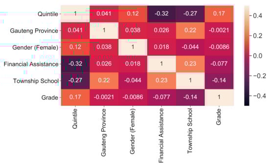
Figure 2.
Pearson Correlation Coefficients of the Chosen Features. Quintile and Township School had the highest correlation with Grade.
Quintile (r = 0.170) had the strongest linear correlation with Grade, followed by Township School ( −0.140). The Background data’s correlations indicate that higher Quintile high-schools generally performed better than students from lower Quintile schools. Students from Township schools performed worse than students from other schools.
Understanding that a relationship exists between the chosen features and Grade showed that these features caould inform the student’s Grade and Outcome.
Classifying a Student Based on Background Data
The classifier used was the Decision Tree Classifier. The train-set contained 3798, while the test-set contained 950 students. The train-test split was stratified by the Outcome of the students. A grid search on the train-set suggested a maximum tree depth of six and eight maximum leaves for the Decision Tree as presented in Table 12.
Table 12.
Confusion matrix and summary of Background–Grade test set results.
If we refer to Table 12, we noted that 640 out of the 950 test observations were classified correctly, producing a of 0.18 (slight agreement) between the Safety Score and the Outcome. The precision score for the Flag students suggested that 107 of the 260 Flagged students were correctly Flagged; the remaining 153 were meant to be Ignored.
3.2. Extraversion-Level and Grade
Although the increase in the mean Grade with Extraversion level was apparent from the line of best-fit, this claim was confirmed by the OLS Regression model’s output in Table 13. The corresponding plot is given in Figure 3. This result showed that students in higher Extraversion levels tended to achieve higher Grades, on average. The fit described in OLS Summary Table 13 showed a linear relationship, . The p-values of 0.000 signified that was not a relationship by chance. Furthermore, the high r of 0.846 signified that moved closely with E and could be inferred from E with a 95% confidence that .
Table 13.
OLS Regression summary—Extraversion level Grade against Extraversion level.
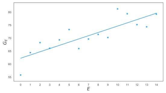
Figure 3.
Extraversion-level Grade against Extraversion-level. , .
Extraversion levels were ordinal, with each level indicating the number of posts in that level. Therefore, an E of one was a lower Extraversion level than an E of two.
3.3. Conscientiousness-Level and Grade
There was a positive relationship between and , with a coefficient p-value of 0.000 as supported by Table 14 and its corresponding plot in Figure 4. An increase of 1 in a student’s Conscientiousness level corresponded to an average increase of 5.988 Grade points out of 100.
Table 14.
OLS regression summary—average number of weekly active days against Grade.
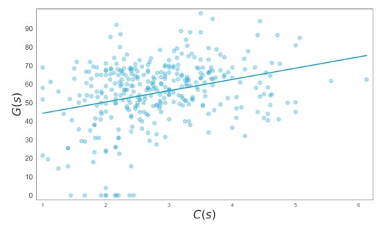
Figure 4.
Average Number of Weekly Active Days against Grade. , .
3.4. Student Discussions and Grade
The OLS Regression Summary for the linear relationship between and in Table 15 showed that the linear equation of the line of best-fit was given by . The corresponding plot is given in Figure 5. The coefficient of and its statistical significance (p = 0.011) indicated that the a marginal increase in of one Grade point corresponded to an average increase of 0.528 in . The of 0.421 indicated a strong correlation between the mean Grade of a Discussion () and the Grade of a student, (), chosen at random, who participated in that Discussion. This correlation also held for any other set of randomly selected students.
Table 15.
OLS regression—random student’s Grades against Discussion’s Grade averages.
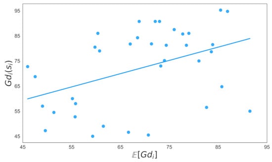
Figure 5.
Random Student’s Grades against Discussion’s Grade Averages. , .
3.5. Student Collaboration—Groups and Grade
Table 16 shows the OLS regression results of the fit between and . The corresponding plot is given in Figure 6.
Table 16.
OLS regression summary—random student’s Grades against Collaboration group’s Grade averages.
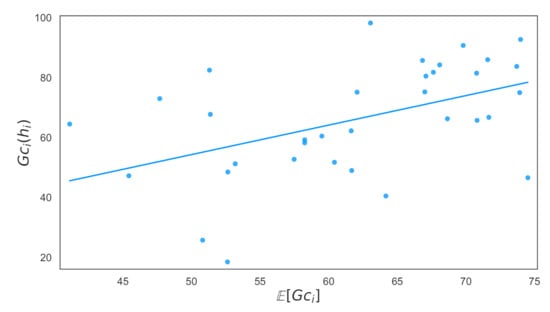
Figure 6.
Random-Student’s Grades against Collaboration-group’s Grade Averages. , .
The coefficient of in Table 16 showed a marginal increase in of one Grade point corresponded to an estimated increase of 0.984 in . The of 0.479 indicates a strong correlation between the average Grade of a Collaboration group——and the Grade of its Host—.
3.6. B-PM and Outcome
Table 17 shows B-PM’s results. The of 0.51 showed a moderate agreement between B-PM’s predicted Safety Scores and actual student Outcomes. B-PM’s precision for the At-risk Outcome group showed that out of the 39 Flagged students, 27 were Flagged correctly (since they ended up at risk of failing). A total of 12 out of the 39 Flagged students were not meant to be Flagged. The At-risk recall indicated that out of 46 At-risk students, 27 were correctly Flagged, and the remaining 19 were incorrectly Ignored.
Table 17.
Confusion matrix and summary of B-PM test set results.
B-PM performed better at classifying Safe students than at classifying At-risk students: only 12 out of 124 Safe students were incorrectly Flagged, and 19 out of 131 Ignored students were wrongly Ignored.
3.7. BM and Outcome
This section reports on the results of a modified model of B-PM without the and input Sequences. The comparison helped determine the change in the accuracy of B-PM after removing its personality components. This resulting model was called the Behaviour Model (BM); the only difference between BM and B-PM is that BM only has one input Sequence, .
Table 18 shows BM’s results. For reference, the comparable B-PM results were shown in brackets. The At-risk recall of BM equalled the At-risk recall of B-PM, meaning that BM correctly Flagged as many At-risk students as B-PM did. BM achieved a of 0.40.
Table 18.
Confusion matrix and summary of BM test set results.
While we only showed B-PM and BM predictions for the end of the 17 weeks, the models also produced predictions at the end of each week. Flagging students at risk earlier may be more beneficial to a student and an institution’s stakeholders since early flagging allows more time for interventions—Section 4.6 reports on the trade-off between timeliness and accuracy.
4. Discussion
4.1. Background and Grade
See Figure 2 and Table 12. Bourdieu and Richardson [26] argue that Cultural and Economic Capital regulates the level of success attainable by individuals. The Pearson correlation coefficients for Grade against Quintile and Township School were 0.17 and −0.14, respectively. The Decision Tree used to classify students at risk produced a of 0.18 (slight agreement) between the Safety Score and the Outcome. The above relationships between Background and a student’s academic output provided evidence for the theories extended by Bourdieu and Richardson [26].
4.2. Extraversion-Level and Grade
See Table 13 and Figure 3. The positive coefficient of 1.269 signified that the average Grade of students in higher Extraversion levels was higher than the average Grade of students in lower Extraversion levels; while one more post than the last may not result in an additional 1.269 points to a student’s Grade record, the average Grade of students who contributed to discussions more frequently, in general, was higher than the Grades of students who posted less often. Although this model accounted for the observed effect on Grade of only one independent variable, Extraversion, the probability (p-value) of Extraversion having no relationship with Grade was 0. This showed a statistical significance of Extraversion as a regressor against student Grade. An increase of 1 in the correlated with an average Grade increase of 1.269. The Extraversion–Grade relationship was linked to the social science concept of social capital for the formation of Academic groups.
4.3. Conscientiousness-Level and Grade
See Table 14 and Figure 4. The coefficient of indicated an increase of 1 in Conscientiousness—level was associated with an increase of 5.988 in Grade. Out of the 102 students who ended up at risk of failing their programmes (Grade ), 76 had a Conscientiousness level below three. The statistically significant positive correlation between and showed that was a suitable predictor of a student’s Outcome.
Hung and Zhang [57] presented a comparable finding; students who accessed course materials 18.5 times or more throughout their programmes obtained a grade of 77.92 out of 100 or higher, while students who accessed course materials more than 44.5 times obtained a grade of 89.62 or higher. Closely related to the above relationship was this study’s findings of the correlation between a student’s Extraversion level, , and Grade.
4.4. Academic Groups and Social Capital
See Table 16 and Figure 6. The Extraversion–Grade relationship was linked to the social science concept of social capital, which was used as a theoretical basis for our formation of Academic groups. Romero et al. [58] obtained a classification accuracy of 60% for the expected grade category of a student (Fail, Pass, Good, Excellent) against their LMS behaviour. Among the features used by Romero et al. [58] was the number of messages sent to a forum (Extraversion level).
Bhandari and Yasunobu [59] and other researchers do not illustrate the quantitative effect of social capital. However, the authors cite that ‘an individual who creates and maintains social capital subsequently gains advantage from it [social capital]’. The quantification of the perceived effect of social capital was illustrated by the correlation between the Grade of a student in an Academic group, , and the average Grade of the group, . responded with a statistically significant increase of 0.984 to a increase of 1.
Despite showing different insights and patterns, both the Discussion and Collaboration group methods showed that the quality of a student’s academic output (Grades) was associated with the quality of the academic output of their social capital. As stated in Section 1.2, a student may choose to leverage their social capital (that is available to all students in a cohort) by becoming part of an Academic group.
Our Academic group and Grade relationship, findings such as Romero et al. [58]’s and the above statement by Bhandari and Yasunobu [59] provide evidence for the positive relationship between student success and the accumulation of social capital. This section’s work contributed to the theory that:
The quality of a student’s social capital is the quality of their Academic group’s performance.
Academic Group Size Constraints
Each Discussion and Collaboration group was constrained to a minimum size of three. When the sizes were reduced to two, all linear relationships between the student’s Grade and the group’s average Grade collapsed and were statistically insignificant. Furthermore, residuals, (for Discussion–Grade relationships) and (for Collaboration group–Grade relationships) were not normally distributed for the group sizes of two.
4.5. BM and B-PM
Work from cited authors does not discuss how changes in student behaviour relate to changes in student performance. Section 3.6 constructed a temporal e-behaviour machine learning model that yielded a of 0.51 against a student’s performance.
4.6. BM and the Trade-Off Waterfall
Figure 7 is a Trade-off Waterfall that illustrates the trade-off between the benefit of intervention timeliness and the cost of intervention success. Intervention success is determined by the model’s accuracy. A red bar represents a decrease in accuracy from one week to the next, and a blue bar indicates an increase. The length of a bar indicates the magnitude of change in accuracy, .
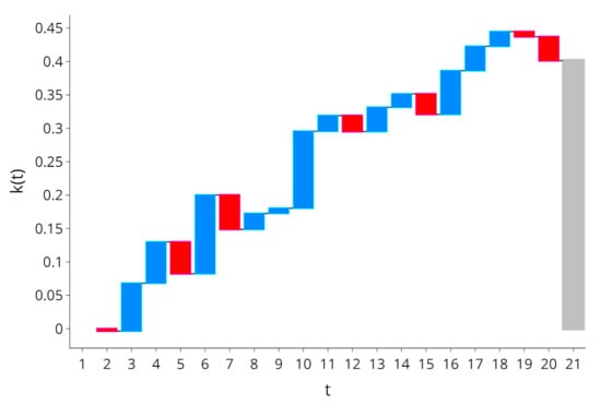
Figure 7.
Trade-off between timeliness and accuracy.
The trade-off between the benefit of intervention timeliness and the cost of intervention success could help identify whether there were patterns over each year that could inform users about the optimal week () to intervene. If the current year was 2019, then for 2019 () could be determined by either one or a combination of the following factors:
- was chosen to be the t in 2018 that yielded the maximum value of in 2018.
- was based on exogenous considerations determined by the institution’s stakeholders. Examples of exogenous considerations were the urgency required for intervention and resources required to make interventions.
For instance, the 2018 Trade-off Waterfall was not available to this study. Therefore, the used in this cohort’s B-PM and BM was based only on the exogenous consideration that interventions should be conducted by week 17.
Practical Benefits and Limitations of the Trade-Off Waterfall
The Trade-off Waterfall was computed after the Outcome of the students was made available. It did not show the week that produced the highest accuracy in real-time, and, in some weeks, the trade-off between accuracy and timeliness was not positive. For example, observe that . In exchange for a delayed intervention, BM produced a worse score from , which would not have made the delay worthwhile. A similar observation was determined for the delay between weeks 18 and 19. Therefore, there was no way to infer the optimal week to make predictions and interventions in real-time. Instead, the Trade-off Waterfall indicated that:
- The general trade-off was that increased as t increased;
- The trade-off peaked at some point, and, in this case, three weeks before the examination period at . Therefore, it may not be worth waiting for the start of an examination period (such as ) before conducting interventions (given the login data of this cohort, different cohorts and different datasets from those presented in this report may produce different peak periods). For example, the Trade-off Waterfall showed that, after , there was no benefit of waiting for an extra one, two or even three weeks to intervene because , , .
5. Limitations and Future Work
This research was a study on the methodology that guided the use of machine learning in an academic performance analysis rather than the efficiency and improvement of the algorithms themselves.
Our results might likely differ across contexts, since different data and algorithm configurations can generate several model outputs. The results obtained serve only as proxies for the possible outputs in academic performance research.
In the domain of an LMS system user engagement, there were no formal definitions and standards, analogues or equivalent metrics that proxied a student’s e-behaviour and personality from LMS data. We modelled features as well-understood traits to further understand the relationships between behaviour, personality and academic performance.
An unknown in all model outcomes was the presence of causality. For instance, whether e-behaviour had an effect on performance was not known. Although the methodology followed aimed to set up conditions for inference, diction such as tend to correspond with, and have relationships with, instead of causes, showed sensitivity to all likelihood of effects from confounding variables.
In encoding performance (student Grade), we used uniform importance across all modules. We did so despite some students’ modules accounting for a higher proportion of points towards obtaining a qualification from the University. We did not have access to each student’s relative weighting of each module and, therefore, did not account for the differences in module weightings.
5.1. Alternative Formulations of Personalities
An approach to capture various facets of Extraversion and Conscientiousness was attempted. For instance, the orderliness facet of Conscientiousness required a metric that modelled the routine or consistency of engagement. Orderliness was modelled by computing the sum of the squared deviations, , from each student’s mean number of logins. However, the regression model that correlated Grades with violated the normality-of-residuals test for normality. Thus, the test for a relationship between and Grade was inappropriate under a linear regression model.
Personality tests, as conducted by Costa et al. [60], could be conducted on students in our study. Using personality assessments as an evaluation tool would help understand the extent to which the proxies we developed corresponded to standard personality assessment procedures and could lead to improved proxies. For example, login behaviour did not capture dutifulness as a personality assessment would. Therefore, responses from the assessments could lead to finding proxies that correlated with Conscientiousness in more ways than dutifulness, providing for a fuller assessment of the Conscientiousness proxy since it would be backed by the existing assessment measures.
5.2. Extraversion Levels
Placing the students in Extraversion levels satisfied the OLS assumptions, while regressing each student’s post count against their Grade produced statistically significant results; the data’s distribution violated OLS assumptions. Hence, the transformation by placing each student into an Extraversion level. Figure 8 shows the Crude Post Count against the Grade of each student. The Residual Normality, Independence, and Homoscedasticity assumptions were violated by the OLS model fitted on the data in Figure 8.
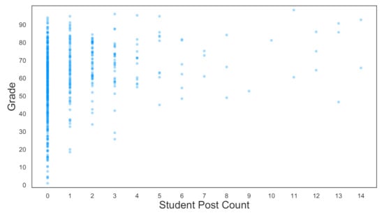
Figure 8.
Crude Post Count against Student Grade. There was a positive relationship between Post Count and Grade that was not suitable for a linear OLS fit.
6. Conclusions
We looked at students’ Background, behaviour, personality and how these factors were related to student performance. The main difference between our methodology and previous work was that we engineered features from an LMS system. We used these LMS features to act as proxy features for e-behaviours and personality traits as an input to our machine learning models. We then analysed the model outputs and their practical implications. The results demonstrated that a student’s background had a lower predictive power of academic performance than their e-behaviour and personality. We found that modelling student behaviours and personality traits required considering how accurately our proposed e-behaviour and personality proxies modelled true behaviours and personality traits—we based our models on definitions found in previous literature.
We were able to use Bourdieu’s Three Forms of Capital to model social, economic and cultural capital, and the Big Five personality traits to model e-behaviour and personality. From student Background and LMS forum engagement data, Bourdieu’s Three Forms of Capital were modelled in the following ways:
- Economic Capital—modelled by the Financial Assistance;
- Cultural Capital—modelled by the Quintile in Province and Township School;
- Social Capital—modelled by Academic groups.
The correlation values for Financial Assistance, Quintile and Township School provided evidence for the authors’ argument that Cultural, Economic and Social Capital regulate the level of success attainable by individuals. Cultural and Economic Capital, combined with the Gender feature, performed better than chance at predicting student performance. A student’s quality of Social Capital available to them also correlated positively with their academic performance.
We used two of the Big Five personality traits, Conscientiousness and Extraversion, previously found to correlate strongly with performance. Conscientiousness and Extraversion each showed significant predictive performance when used in our MNL models. With these personality features, our e-behaviour classifier achieved better accuracy than without the personality features. The works cited do not discuss how changes in student behaviour relate to changes in their performance. We constructed a temporal e-behaviour model using deep learning that showed an increase in accuracy over time. This e-behaviour learning can be used to flag students at risk at any point throughout their study programmes.
The analyses in this research could be practically useful if they could inform or influence student behaviour. Firstly, a student may find helpful the linear relationship between academic performance and Extraversion. The empirical evidence that a higher Extraversion level is associated with a better academic performance may encourage students to engage in forums more frequently. This evidence may encourage them to engage with the academic content more thoroughly to contribute meaningfully to discussions. Secondly, we showed, using unsupervised cluster learning, that a student’s performance was congruent with the performance of their Academic group. The above result is a further motive to action a student into leveraging their social capital by engaging in forums more frequently, since engagement increases their chances of being in an Academic group.
Author Contributions
Conceptualization, S.B.-W.S., R.K. and T.v.Z.; Data curation, S.B.-W.S.; Formal analysis, S.B.-W.S.; Funding acquisition, R.K. and T.v.Z.; Investigation, S.B.-W.S., R.K. and T.v.Z.; Methodology, S.B.-W.S.; Supervision, R.K. and T.v.Z.; Validation, S.B.-W.S.; Visualization, S.B.-W.S.; Writing—original draft, S.B.-W.S., R.K. and T.v.Z.; Writing—review & editing, S.B.-W.S., R.K. and T.v.Z. All authors have read and agreed to the published version of the manuscript.
Funding
The APC was funded by National Research Foundation, South Gate, Meiring Naudé Road, Tshwane, South Africa.
Institutional Review Board Statement
This research filed for a study ethics application that was approved by the Human Research Ethics Committee at the University of the Witwatersrand, Johannesburg, South Africa, 2001. The ethics application included measures imposed on the research methodology to ensure the protection of the student identities and their data’s security. This research’s clearance certificate protocol number is H19/06/36.
Conflicts of Interest
The funders had no role in the design of the study; in the collection, analyses, or interpretation of data; in the writing of the manuscript, or in the decision to publish the results.
References
- Richiţeanu-Năstase, E.R.; Stăiculescu, C. University dropout. Causes and solution. Ment. Health Glob. Chall. J. 2018, 1, 71–75. [Google Scholar]
- Wright, D.; Taylor, A. Introducing Psychology: An Experimental Approach; Penguin Books: London, UK, 1970. [Google Scholar]
- Heppner, P.P.; Wampold, B.E.; Owen, J.; Wang, K.T.; Thompson, M.N. Research Design in Counseling, 4th ed.; Cengage Learning: Boston, MA, USA, 2015. [Google Scholar]
- Stone, A.A. Hove, East Sussex, United Kingdom; Lawrence Erlbaum: Mahwah, NJ, USA, 2000. [Google Scholar]
- Northrup, D.A.; York University (Toronto, O.; for Social Research, I.). The Problem of the Self-Report in Survey Research: Working Paper; Institute for Social Research, York University: North York, ON, Canada, 1997. [Google Scholar]
- Fellegi, I.P. The Evaluation of the Accuracy of Survey Results: Some Canadian Experiences. Int. Stat. Rev. Rev. Int. Stat. 1973, 41, 1–14. [Google Scholar] [CrossRef]
- Costa, P.T.; McCrae, R.R. The NEO Personality Inventory; Psychological Assessment Resources: Odessa, FL, USA, 1985. [Google Scholar]
- Poropat, A.E. A meta-analysis of the five-factor model of personality and academic performance. Psychol. Bull. 2009, 135, 322. [Google Scholar] [CrossRef] [Green Version]
- Furnham, A.; Nuygards, S.; Chamorro-Premuzic, T. Personality, assessment methods and academic performance. Instr. Sci. 2013, 41, 975–987. [Google Scholar] [CrossRef]
- Ciorbea, I.; Pasarica, F. The study of the relationship between personality and academic performance. Procedia-Soc. Behav. Sci. 2013, 78, 400–404. [Google Scholar] [CrossRef] [Green Version]
- Kumari, B. The correlation of Personality Traits and Academic performance: A review of literature. IOSR J. Humanit. Soc. Sci. 2014, 19, 15–18. [Google Scholar] [CrossRef]
- Morris, P.E.; Fritz, C.O. Conscientiousness and procrastination predict academic coursework marks rather than examination performance. Learn. Individ. Differ. 2015, 39, 193–198. [Google Scholar] [CrossRef] [Green Version]
- Chamorro-Premuzic, T.; Furnham, A. Personality predicts academic performance: Evidence from two longitudinal university samples. J. Res. Personal. 2003, 37, 319–338. [Google Scholar] [CrossRef]
- Kim, S.; Fernandez, S.; Terrier, L. Procrastination, personality traits, and academic performance: When active and passive procrastination tell a different story. Personal. Individ. Differ. 2017, 108, 154–157. [Google Scholar] [CrossRef] [Green Version]
- Costa, P.T., Jr.; McCrae, R.R. The Revised NEO Personality Inventory (NEO-PI-R); Sage Publications, Inc.: Newbury Park, CA, USA, 2008. [Google Scholar]
- Wilt, J.; Revelle, W. Extraversion. In Handbook of Individual Differences in Social Behavior; The Guilford Press: New York, NY, USA, 2009; pp. 27–45. [Google Scholar]
- APA Dictionary of Psychology–Gregariousness. 2020. Available online: https://dictionary.apa.org/gregariousness (accessed on 29 December 2020).
- Merriam-Webster. Dutiful. Available online: https://www.merriam-webster.com/dictionary/dutifulness (accessed on 29 November 2020).
- Akçapınar, G. Profiling students’ approaches to learning through moodle logs. In Proceedings of the Multidisciplinary Academic Conference on Education, Teaching and Learning (MAC-ETL 2015), Prague, Czech Republic, 4–6 December 2015. [Google Scholar]
- Huang, A.Y.; Lu, O.H.; Huang, J.C.; Yin, C.J.; Yang, S.J. Predicting students’ academic performance by using educational big data and learning analytics: Evaluation of classification methods and learning logs. Interact. Learn. Environ. 2020, 28, 206–230. [Google Scholar] [CrossRef]
- Khan, I.A.; Brinkman, W.P.; Fine, N.; Hierons, R.M. Measuring personality from keyboard and mouse use. In Proceedings of the 15th European Conference on Cognitive Ergonomics: The Ergonomics of Cool Interaction, Funchal, Portugal, 16–19 September 2008; pp. 1–8. [Google Scholar]
- Fowler, G.C.; Glorfeld, L.W. Predicting aptitude in introductory computing: A classification model. AEDS J. 1981, 14, 96–109. [Google Scholar] [CrossRef]
- Poh, N.; Smythe, I. To what extend can we predict students’ performance? A case study in colleges in South Africa. In Proceedings of the 2014 IEEE Symposium on Computational Intelligence and Data Mining (CIDM), Orlando, FL, USA, 9–12 December 2014; pp. 416–421. [Google Scholar] [CrossRef]
- Evans, G.E.; Simkin, M.G. What Best Predicts Computer Proficiency? Commun. ACM 1989, 32, 1322–1327. [Google Scholar] [CrossRef]
- Dauter, L.G. Economic Sociology. 2016. Available online: https://www.britannica.com/topic/economic-sociology (accessed on 29 December 2020).
- Bourdieu, P.; Richardson, J.G. The forms of capital. In Cultural Theory: An Anthology; John Wiley & Sons: Hoboken, NJ, USA, 1986. [Google Scholar]
- Carpiano, R.M. Toward a neighborhood resource-based theory of social capital for health: Can Bourdieu and sociology help? Soc. Sci. Med. 2006, 62, 165–175. [Google Scholar] [CrossRef] [PubMed]
- Hallinan, M.T.; Smith, S.S. Classroom characteristics and student friendship cliques. Soc. Forces 1989, 67, 898–919. [Google Scholar] [CrossRef]
- Song, L. Social capital and psychological distress. J. Health Soc. Behav. 2011, 52, 478–492. [Google Scholar] [CrossRef] [PubMed]
- Hayes, E. Elaine Hayes on “The Forms of Capital”. 1997. Available online: https://web.english.upenn.edu/~jenglish/Courses/hayes-pap.html (accessed on 2 November 2021).
- Smith, E.; White, P. What makes a successful undergraduate? The relationship between student characteristics, degree subject and academic success at university. Br. Educ. Res. J. 2015, 41, 686–708. [Google Scholar] [CrossRef] [Green Version]
- Caldas, S.J.; Bankston, C. Effect of School Population Socioeconomic Status on Individual Academic Achievement. J. Educ. Res. 1997, 90, 269–277. [Google Scholar] [CrossRef]
- Fan, J. The Impact of Economic Capital, Social Capital and Cultural Capital: Chinese Families’ Access to Educational Resources. Sociol. Mind 2014, 4, 272–281. [Google Scholar] [CrossRef] [Green Version]
- Ajzen, I. Attitudes, Personality, and Behavior; McGraw-Hill Education: New York, NY, USA, 2005. [Google Scholar]
- Campbell, D.T. Social Attitudes and Other Acquired Behavioral Dispositions. In Psychology: A Study of a Science. Study II. Empirical Substructure and Relations with Other Sciences. Investigations of Man as Socius: Their Place in Psychology and the Social Sciences; McGraw-Hill: New York, NY, USA, 1963; Volume 6, pp. 94–172. [Google Scholar] [CrossRef]
- Hemakumara, G.; Ruslan, R. Spatial Behaviour Modelling of Unauthorised Housing in Colombo, Sri Lanka. KEMANUSIAAN Asian J. Humanit. 2018, 25, 91–107. [Google Scholar] [CrossRef]
- Guyon, I.; Weston, J.; Barnhill, S.; Vapnik, V. Gene selection for cancer classification using support vector machines. Mach. Learn. 2002, 46, 389–422. [Google Scholar] [CrossRef]
- Barrick, M.R.; Mount, M.K.; Strauss, J.P. Conscientiousness and performance of sales representatives: Test of the mediating effects of goal setting. J. Appl. Psychol. 1993, 78, 715. [Google Scholar] [CrossRef]
- Campbell, J.P. Modeling the performance prediction problem in industrial and organizational psychology. In Handbook of Industrial and Organizational Psychology; Consulting Psychologists Press: Palo Alto, CA, USA, 1990. [Google Scholar]
- Stigler, S.M. Gauss and the Invention of Least Squares. Ann. Stat. 1981, 9, 465–474. [Google Scholar] [CrossRef]
- Blumberg, M.; Pringle, C.D. The missing opportunity in organizational research: Some implications for a theory of work performance. Acad. Manag. Rev. 1982, 7, 560–569. [Google Scholar] [CrossRef]
- Leontjeva, A.; Kuzovkin, I. Combining Static and Dynamic Features for Multivariate Sequence Classification. In Proceedings of the 2016 IEEE International Conference on Data Science and Advanced Analytics (DSAA), Montreal, QC, Canada, 17–19 October 2016; pp. 21–30. [Google Scholar] [CrossRef] [Green Version]
- Safavian, S.R.; Landgrebe, D. A survey of decision tree classifier methodology. IEEE Trans. Syst. Man Cybern. 1991, 21, 660–674. [Google Scholar] [CrossRef] [Green Version]
- Mitchell, T.M. Machine Learning, 1st ed.; McGraw-Hill, Inc.: New York, NY, USA, 1997; Chapter 10. [Google Scholar]
- Raileanu, L.; Stoffel, K. Theoretical Comparison between the Gini Index and Information Gain Criteria. Ann. Math. Artif. Intell. 2004, 41, 77–93. [Google Scholar] [CrossRef]
- Khalaf, A.; Hashim, A.; Akeel, W. Predicting Student Performance in Higher Education Institutions Using Decision Tree Analysis. Int. J. Interact. Multimed. Artif. Intell. 2018, 5, 26–31. [Google Scholar]
- Topîrceanu, A.; Grosseck, G. Decision tree learning used for the classification of student archetypes in online courses. Procedia Comput. Sci. 2017, 112, 51–60. [Google Scholar] [CrossRef]
- Kolo, K.D.; Adepoju, S.A.; Alhassan, J.K. A decision tree approach for predicting students academic performance. Int. J. Educ. Manag. Eng. 2015, 5, 12. [Google Scholar] [CrossRef] [Green Version]
- Gujarati, D.N.; Porter, D.C. Basic Econometrics; McGraw Hill Inc.: New York, NY, USA, 2009. [Google Scholar]
- Liu, Z.; Sullivan, C.J. Prediction of weather induced background radiation fluctuation with recurrent neural networks. Radiat. Phys. Chem. 2019, 155, 275–280. [Google Scholar] [CrossRef]
- Wang, M.; Zhang, Y.D.; Cui, G. Human motion recognition exploiting radar with stacked recurrent neural network. Digit. Signal Process. 2019, 87, 125–131. [Google Scholar] [CrossRef]
- Bengio, Y.; Boulanger-Lewandowski, N.; Pascanu, R. Advances in Optimizing Recurrent Networks. In Proceedings of the 2013 IEEE International Conference on Acoustics, Speech and Signal Processing, Vancouver, BC, Canada, 26–31 May 2013. [Google Scholar]
- Olah, C. Understanding LSTM Networks. 2015. Available online: https://colah.github.io/posts/2015-08-Understanding-LSTMs/ (accessed on 19 April 2019).
- Hand, D.; Christen, P. A note on using the F-measure for evaluating record linkage algorithms. Stat. Comput. 2018, 28, 539–547. [Google Scholar] [CrossRef] [Green Version]
- Cohen, J. A Coefficient of Agreement for Nominal Scales. Educ. Psychol. Meas. 1960, 20, 37–46. [Google Scholar] [CrossRef]
- Landis, J.R.; Koch, G.G. The measurement of observer agreement for categorical data. Biometrics 1977, 33, 159–174. [Google Scholar] [CrossRef] [Green Version]
- Hung, J.L.; Zhang, K. Revealing online learning behaviors and activity patterns and making predictions with data mining techniques in online teaching. MERLOT J. Online Learn. Teach. 2009, 4, 426–437. [Google Scholar]
- Romero, C.; Ventura, S.; Espejo, P.; Martínez, C. Data Mining Algorithms to Classify Students; Journal of Education and Data Mining: Memphis, TN, USA, 2008; pp. 8–17. [Google Scholar]
- Bhandari, H.; Yasunobu, K. What Is Social Capital? A Comprehensive Review of the Concept. Asian J. Soc. Sci. 2009, 37, 480–510. [Google Scholar] [CrossRef]
- Costa, P.; McCrae, R.; Kay, G. Persons, Places, and Personality: Career Assessment Using the Revised NEO Personality Inventory. J. Career Assess. 1995, 3, 123–139. [Google Scholar] [CrossRef]
Publisher’s Note: MDPI stays neutral with regard to jurisdictional claims in published maps and institutional affiliations. |
© 2021 by the authors. Licensee MDPI, Basel, Switzerland. This article is an open access article distributed under the terms and conditions of the Creative Commons Attribution (CC BY) license (https://creativecommons.org/licenses/by/4.0/).