Illuminant Estimation Using Adaptive Neuro-Fuzzy Inference System

Abstract

Computational color constancy (CCC) is a fundamental prerequisite for many computer vision tasks. The key of CCC is to estimate illuminant color so that the image of a scene under varying illumination can be normalized to an image under the canonical illumination. As a type of solution, combination algorithms generally try to reach better illuminant estimation by weighting other unitary algorithms for a given image. However, due to the diversity of image features, applying the same weighting combination strategy to different images might result in unsound illuminant estimation. To address this problem, this study provides an effective option. A two-step strategy is first employed to cluster the training images, then for each cluster, ANFIS (adaptive neuro-network fuzzy inference system) models are effectively trained to map image features to illuminant color. While giving a test image, the fuzzy weights measuring what degrees the image belonging to each cluster are calculated, thus a reliable illuminant estimation will be obtained by weighting all ANFIS predictions. The proposed method allows illuminant estimation to be dynamic combinations of initial illumination estimates from some unitary algorithms, relying on the powerful learning and reasoning capabilities of ANFIS. Extensive experiments on typical benchmark datasets demonstrate the effectiveness of the proposed approach. In addition, although there is an initial observation that some learning-based methods outperform even the most carefully designed and tested combinations of statistical and fuzzy inference systems, the proposed method is good practice for illuminant estimation considering fuzzy inference eases to implement in imaging signal processors with if-then rules and low computation efforts.

1. Introduction

The human vision system has the instinctive ability to perceive true color even under some specific imaging conditions and scene illumination. This “color constancy” capability for computer systems is becoming more and more necessary due to a wide range of computer vision applications [1,2]. Unfortunately, without specific algorithms, computers and imaging sensors in modern digital cameras do not innately possess this capability. To address this issue, a variety of computational color constancy (CCC) algorithms have been proposed, aiming to endow computers with super power to compensate for the effect of the illumination on objects’ color perception.

Generally, CCC works with two steps: first obtaining an estimate of illuminant color, and then correcting color deviations by multiplying the reciprocal of the illuminant color to the color-biased image [1,2,3]. The first step, i.e., illuminant estimation, is the key.

To date, there are many approaches proposed by various researchers to solve the illuminant estimation issue. These methods can be roughly categorized into three groups: statistics-based, learning-based, and combinational. Statistics-based methods are based on some statistical features that are kept consistent in the image captured under canonical light conditions, e.g., Gray world (GW) [4,5], White patch (WP) [6], Shades of gray (SoG) [7], Gray edge (GE) [8], etc. Learning-based algorithms have a learning phase and use various image information, normally low-level image features, to pre-train models to estimate the illuminant color, e.g., natural image statistics [9], classification-based algorithm selection [10], deep learning based methods [11,12,13,14,15,16], etc. The first two types of algorithms, called unitary algorithms, use a single strategy, and usually can not balance among implementation cost, computation efforts, and algorithm complexity. In contrast, the third group, called combination methods, may use multiple unitary strategies to estimate initial illumination and then combine the resulting estimates in some way to form a robust estimate [17].

Combination methods try to reach better results by weighting other algorithms or selecting the best algorithm for a given image [18,19]. In weighting combination related methods, the weights for the combination of unitary algorithms might be static or dynamic. Due to the difficulty to finding static parameters to efficiently combine a wide range of real-world images, dynamic weights are normally introduced to fit the changes in various image features. Nevertheless, it is also hard to formulate dynamic weighting schemes to combine unitary algorithms [19,20]. Alternatively, an available option is to first classify a test image into a certain class using a pre-trained multi-class classifier and then determine appropriate unitary algorithms to estimate illumination. However, in most attempts, the image classification accuracy is not satisfactory [19], although many different schemes are designed [18,21,22].

In this paper, leveraging the powerful computation, learning, and inference abilities of ANFIS (adaptive neuro-network fuzzy inference system), we propose an ANFIS based multiple model approach for illuminant estimation. The contributions of this work are as follows. (1) A two-step clustering strategy is developed to group the training dataset, the first step based on color distribution features, the second based on initial illumination estimates from unitary algorithms. This conduction will result in better clustering division that fits for illuminant estimation modeling. (2) Multiple ANFIS model structures are effectively used to regress the underlying relationship between initial illuminant estimates and illuminant color, which can automatically learn model parameters and significantly improve the estimation performance. (3) With adaptive weight computations, we provide a general method to weight all predictive outputs from ANFIS models.

The rest of the paper is organized as follows. The related works are discussed in Section 2. The proposed framework is presented in Section 3, in which feature extraction, image clustering, ANFIS modeling, and illuminant estimation are exploited in details. Afterwards, in Section 4 we validate our proposed method with some experimental results and give some further discussions. Finally, we conclude the work in Section 5.

2. Related Works

In this section, we give a brief introduction to statistics-based and combination methods, since our proposed method is mainly with respect to both of them.

Statistics based methods. These algorithms directly compute some statistical measures of the input image to estimate illuminant color without complicated computational effort, although sometimes the accuracy cannot be assured. Most of these algorithms can be unified into a GE framework developed by Weijer et al. [23], which includes higher-order derivatives and the Minkowski family norm given as:

$${\left({\displaystyle \int }{\left|\frac{{\partial }^n{\mathbf{f}}^{\sigma }\left(\mathbf{x}\right)}{\partial {\mathbf{x}}^n}\right|}^{p}d\mathbf{x}\right)}^{\frac{1}{p}}=k{\mathbf{e}}^{n,p,\sigma },$$

(1)

Here ${\mathbf{f}}^{\sigma }=\mathbf{f}\otimes {\mathbf{G}}^{\sigma }$ denotes convolution of the image with a norm value, k is a scaling, and $e^{n,p,\sigma }$ is the resulting illuminant estimate. The methods defined by different choices of the parameters n, p and $\sigma$ are denoted as $G{E}^{n,p,\sigma }$, where the optimal values of these parameters may vary with different datasets. Some assumptions based algorithms are special instantiations of this framework [18,20,23,24], WP and GW also being included: (1) GW ($G{E}^{0,1,0}$); (2) WP ($G{E}^{0,\infty ,0}$); (3) SoG ($G{E}^{0,6,0}$); (4) 1-order gray edge (GE1) ($G{E}^{1,1,6}$); (5) 2-order gray edge (GE2) ($G{E}^{2,1,5}$); (6) General gray world (GGW) ($G{E}^{0,13,2}$).

The other examples of statistics based methods include bright-and-dark color PCA (PCA-based) and local surface reflection (LSR) methods. The PCA-based method proposed by Cheng and Brown [25] selects the color points with largest and smallest projections on the mean chromaticity, and then calculates its first PCA vector as the illuminant estimation. This method is fairly efficient and easy to compute. Gao et al. [26] found that the ratio of the global summation of true surface reflectance to the global summation of locally normalized reflectance estimate in a scene is approximately achromatic for both indoor and outdoor scenes. Based on this substantial observation, LSR illuminant estimation model is developed which has only one free parameter and requires no explicit training process.

Combination methods. Let $E=\{e_1,e_2,\cdots \}$ be the set of the illumination estimates obtained from some statistics or learning based unitary algorithms, then combination methods are to combine the estimates $e_1$,$e_2,\cdots$ into a single, final estimate by corresponding weights $w_1$,$w_2,\cdots$. According to whether $w_1$,$w_2,\cdots$ are constant or not, combination methods can be divided into two basic groups, i.e., static weight combination and dynamic weight combination. Static weights commonly are not suitable for the diversity of image characteristics; the related methods [18,27], like Simple Averaging, Nearest-N%, and Median, etc., can not obtain robust illuminant estimation. On the other hand, dynamic weights vary with image features to guide the selection or combination of unitary estimates [10,11,18]. Various scene characteristics, including low-level properties (e.g., visual properties [10], 3D geometry [28,29]), mid-level initial illumination estimates [30], high-level semantic content (e.g., semantic likelihood [31], indoor/outdoor classification [9]), can be used to find the best combination. Furthermore, the weights might be obtained by different algorithms, such as machine learning [19,32,33,34], Fuzzy model [24], multi-objective optimization [20], graph-based semi-supervised [30], or one without prior training [9,21]. In most combination methods, weight determination is usually accompanied by image classification and training regression models for different classes in order to deal with a wide range of image features [19]. It is a significant obstacle to reach better performances for combination algorithms.

3. Proposed Method

Given an input image, that is in the linear RGB space of a camera after removing black level and saturation level, the proposed method is to estimate a 3D vector as $\widehat{\ell }={[{\widehat{\ell }}_R,{\widehat{\ell }}_G,{\widehat{\ell }}_B]}^T$ that represents the scene illuminant color for this image. An overview of the proposed method is illustrated in Figure 1.

As shown in Figure 1, the training phase contains three major steps: feature extraction, image clustering, and ANFIS modeling. By a two-step clustering strategy, training images are classified into different clusters according to color distribution features (CDFs) and initial illumination features (IIFs). Then multiple ANFIS models are effectively trained to regress the underlying relationship between image features and illuminant. In the testing phase, CDFs and IIFs will be extracted and the corresponding combination weights will be calculated dynamically. The final illuminant estimation is obtained by fuzzy weighting all outputs of ANFIS models.

3.1. Features Extraction

3.1.1. CDF Extraction

Since the color distribution is one of key spatial-domain information which is most related to illuminant estimation, in this study we extract several types of CDFs from an image.

Number of colors. The color number in an image can be used to indicate the color range of the image. We use a number of colors, $n^c$, for the re-quantized image with 6-bits each channel [20] as the first component in the CDFs of the proposed approach.

Chromaticity features. Let R, G, and B be Red, Green, and Blue measurements of an image pixel, the chromaticity values, r and g, are calculated as follows:

$$\left\{\begin{array}{c}r=R/\left(R+G+B\right)\\ g=G/\left(R+G+B\right)\end{array}\right.$$

(2)

We use four chromaticity features in the prior work [35] as follows.

Average color chromaticity is the chromaticity $(r^a,g^a)$ of the average RGB value $(R^a,G^a,B^a)$, where:

$$C^a=\frac{1}{n}\sum _{i=1}^n{C}_i,C\in \left\{R,G,B\right\},$$

(3)

n is the pixel number in the image, and $C^a$ is the channel average same with GW algorithm.

Brightest color chromaticity is the chromaticity $(r^b,g^b)$ of the color $(R^b,G^b,B^b)$ of the pixel k which has the largest brightness value of $(R+G+B)$, i.e.,:

$$\left(R^b,G^b,B^b\right)=\left(R_k,G_k,B_k\right),wherek=\underset{i}{argmax}\left(R_i+G_i+B_i\right).$$

(4)

This differs from WP algorithm that treats each RGB channels independently.

Dominant chromaticity is the chromaticity $(r^d,g^d)$ of the average RGB color $(R^d,G^d,B^d)$ of the pixels belonging to a histogram bin, which has the largest count:

$$C^d=\frac{1}{\left|H_k\right|}\sum _{j\in H_k}{C}_j,C\in \left\{R,G,B\right\},wherek=\underset{i}{\mathrm{argmax}}\left|H_i\right|,$$

(5)

where $H_m$ is the set of pixels in the m-th bin of the histogram.

Chromaticity mode in this study refers to the mode of the image color palette in chromaticity space. The color palette is generated by taking the average value of each bin in the RGB histogram that includes more than a predefined threshold of pixels [35]. A threshold of 200 pixels per bin is set in this study, which yields a palette of approximately 300 colors for a typical image. Each color in the palette is projected onto the normalized chromaticity plane, and an efficient 2D kernel density estimation is performed. The mode $(r^m,g^m)$ is assigned to be the chromaticity with the highest density.

Color moments are some measures to characterize color distribution in an image. If the color in an image follows a certain probability distribution, the moments of that distribution can then be used as the features to identify that image based on color. Since color information is mainly distributed in low-order moments, it is sufficient to use three central moments to express the color distribution of the image, i.e., 1-order moments (Mean), 2-order moments (Standard deviation), and 3-order moments (Skewness). Let $C_i,C\in \left\{R,G,B\right\}$ represent the color component of the i-th pixel of an image, and n be the number of pixels in the image, then the three color moments can be defined as follows respectively:

$${\mu }_C=\frac{1}{n}\sum _{i=1}^n{C}_i,$$

(6)

$${\sigma }_C={(\frac{1}{n}\sum _{i=1}^n{\left(C_i-{\mu }_C\right)}^2)}^{\frac{1}{2}},$$

(7)

$$s_C={(\frac{1}{n}\sum _{i=1}^n{\left(C_i-{\mu }_C\right)}^3)}^{\frac{1}{3}}.$$

(8)

Considering the image size, in this paper we evenly divide an image into $3\times 3$ sub-blocks, and nine moments will be calculated for each sub-block. Therefore, the image is characterized by 27 moments for each 3 color channels, i.e., in total 81 moments such as ${\phi }_1,{\phi }_2,\cdots ,{\phi }_{81}$.

Thus, for an image I in a training dataset, we can obtain all above-mentioned CDFs of this image and formulate them into a CDF vector as follows:

$$\varphi \left(I\right)=[{\lambda }_1{n}^c,{\lambda }_2{r}^a,{\lambda }_2{g}^a,{\lambda }_2{r}^b,{\lambda }_2{g}^b,{\lambda }_2{r}^d,{\lambda }_2{g}^d,{\lambda }_2{r}^m,{\lambda }_2{g}^m,{\lambda }_3{\phi }_1,{\lambda }_3{\phi }_2,\cdots ,{\lambda }_3{\phi }_{81}],$$

(9)

where ${\lambda }_i,i=1,2,3$, represents the influence factor for the corresponding CDF component. Denoting the image number of the training dataset as N, a CDF matrix for the training dataset is obtained as:

$$\Phi ={\left[\begin{array}{cccc}\varphi {}^T\left(I_1\right)& \varphi {}^T\left(I_2\right)& \cdots & \varphi {}^T\left(I_N\right)\end{array}\right]}^T.$$

(10)

3.1.2. Dimensionality Reduction

In this study, Primary Component Analysis (PCA) algorithm is used for dimensionality reduction. Applying PCA, the $\Phi$ matrix from Equation (10) is decomposed to determine a set of loading vectors by singular decomposition [36]. Then the observations in $\Phi$ can be projected into the lower dimensional score matrix, T, which is given as

$$T=\Phi P,$$

(11)

where $P\in {\Re }^{m\times q}$ includes the loading vectors corresponding to the first q largest singular values.

Finally, the PCA feature vector for a given image I is computed as follows:

$$\overline{\varphi }\left(I\right)=(\varphi \left(I\right)-b)P,$$

(12)

where $\overline{\varphi }\left(I\right)\in {\Re }^q$ contains q principal component (PC) coefficients, $P=[p_1,p_2,\cdots ,p_q]$, $p_i\in {\Re }^m$, is the PC coefficient matrix computed by the singular value decomposition, and $b\in {\Re }^m$ is the mean vector of $\Phi$, $b=mean(\Phi )$. Here $m=90$, and q can be manually set or automatically chosen by the percent variability of principal components. As a result, the CDFs of an image I can be represented by a compact vector $\overline{\varphi }\left(I\right)$ that consists of a small number of PC coefficients. Therefore, the compact CDF matrix for the training dataset will be produced as:

$$\overline{\Phi }={\left[\begin{array}{cccc}{\overline{\varphi }}^T\left(I_1\right)& {\overline{\varphi }}^T\left(I_2\right)& \cdots & {\overline{\varphi }}^T\left(I_N\right)\end{array}\right]}^T.$$

(13)

3.1.3. IIF Extraction

For any image in the training dataset, the eight conventional unitary algorithms are applied to get illuminant color vectors $e_i=[R_i,G_i,B_i]$. Here the subscripts $i=1,2,\cdots ,8$ represent the unitary algorithms described in Section 2, i.e., GW, WP, SoG, GE1, GE2, GGW, PCA-based, and LSR, respectively. These methods are based on different principles to estimate illumination; each method is suitable for some specific image types to achieve better estimation accuracy, but might not be suitable for other image types. Commonly, for a given image, different vectors $e_i$ have different values, and sometimes the differences between two of them are significant. Thus we can consider $e_i$ as a certain metric under corresponding hypothesis. For example, $e_1=[R_1,G_1,B_1]$ can be regarded as a metric under the GW assumption. Consequently, we can construct an integrated IIF vector for an image I as follows:

$$\theta \left(I\right)=\left[\gamma (e_i,e_j)\right],i=1,2,\cdots ,8,j=(i+1),(i+2),\cdots ,8,$$

(14)

where $\gamma (e_i,e_j)$ is defined as Euclide distance between $e_i$ and $e_j$ in 3D color space.

Since we just consider illuminant color, rather than illumination intensity, we take Equation (2) to compute the chromaticity $(r_i,g_i)$ for the illuminant color vector $e_i,i=1,2,\cdots ,8$. Alternatively, we may construct another type of integrated IIF vector for an image I as follows:

$$\theta \left(I\right)=[r_1,g_1,r_2,g_2,r_3,g_3,r_4,g_4,r_5,g_5,r_6,g_6,r_7,g_7,r_8,g_8].$$

(15)

Denoting the image number in the training dataset as N, an IIF matrix for the training dataset is obtained as follows:

$$\Theta ={\left[\begin{array}{cccc}\theta {}^T\left(I_1\right)& \theta {}^T\left(I_2\right)& \cdots & \theta {}^T\left(I_N\right)\end{array}\right]}^T.$$

(16)

3.2. Image Clustering

In this stage, a two-step clustering is conducted and all the training images are effectively classified into a few small clusters. The clustering procedure uses k-means algorithm, since this algorithm has straightforward implementation and fast convergence.

Clustering based on CDF. In the two-step strategy, the first step is to cluster the training data into $k_1$ clusters based on CDFs of all training images. Usually, the cluster number for k-means algorithm should be set in advance, or be searched by a certain optimal method like PSO (particle swarm optimization). In this study, we empirically chose $k_1$ through many effective experiments on the training dataset. K-means algorithm is implemented based on iteration procedure. The starting points are provided by initial estimates of some centroids which are randomly selected from the dataset. The algorithm alternately iterates between assigning data points and updating centroids. During the iteration, the data point is assigned to its nearest centroid based on the squared Euclidean distance.

After the k-means clustering based on CDF, the observations of the data matrix $\overline{\Phi }$ obtained via Equation (13) are partitioned into $k_1$ clusters, and the algorithm finally returns an N-by-1 vector containing cluster indices of each observation. According to the cluster indices, each image in the training dataset should fall into $k_1$ subsets as follows:

$$S_i=\{I_{i,1},I_{i,2},\cdots ,I_{i,n_i}\},i=1,2,\cdots ,k_1,$$

(17)

where $n_i$ is the number of images in cluster $S_i$, and ${\sum }_{i=1}^{k_1}{n}_i=N$. It should be noted that the value of $n_i$ maybe different for different clusters. Representing the cluster centroid of $S_i$ as $c_i,i=1,2,\cdots ,k_1$, the CDF centroid set is obtained as $C_{cdf}=\{c_1,c_2,\cdots ,c_{k_1}\}$. The squared Euclidean distance between the CDF vector $\overline{\varphi }\left(I\right)$ of a given image and a cluster centroid $c_i$ can be calculated, which will be used to measure what degree an image belongs to cluster $S_i$.

Clustering based on IIF. In the two-step clustering, the second step is to classify each $S_i$ of the training data into some sub-clusters based on IIFs of all training images. For simplicity, we divide each cluster $S_i$ into the same number of sub-clusters, denoted as $k_2$. As if the clustering is based on CDF, we use the k-means algorithm and still empirically chose the cluster number $k_2$ through many experiments (The optimal values of $k_1$ and $k_2$ should be explored by testing experiments that will be discussed in Section 4.4). In each clustering for $S_i$, the starting points for iteration are randomly selected from the corresponding image set of $S_i$. However, during the iteration the data point is assigned to its nearest centroid based on the cosine distance, not based on the squared Euclidean distance like in CDF based clustering.

For cluster $S_i$, an IIF matrix ${\Theta }_i$ is obtained as in Equation (16). Applying the k-means algorithm, the observations of ${\Theta }_i$ are partitioned into $k_2$ clusters. The algorithm returns a $k_2$-by-1 vector containing the cluster indices. According to the cluster indices, all images in cluster $S_i$ are split into $k_2$ subsets. This results in that the total cluster number for all training images equals $k_1·k_2$. Finally, for the entire training dataset, there are $k_1·k_2$ clusters as follows:

$$S{S}_{ij}=\{I_{ij,1},I_{ij,2},\cdots ,I_{ij,n_{ij}}\},i=1,2,\cdots ,k_1,j=1,2,\cdots ,k_2,$$

(18)

where $n_{ij}$ is the number of images in cluster $S{S}_{ij}$, and ${\sum }_{i=1}^{k_1}{\sum }_{j=1}^{k_2}{n}_{ij}=N$. Representing the cluster centroid of $S{S}_{ij}$ as $c_{ij}$, the IIF centroid set is obtained as $C_{iif}=\{c_{ij},i=1,2,\cdots ,k_1,j=1,2,\cdots ,k_2\}$. The cosine distance between the IIF vector $\theta \left(I\right)$ of a given image and a cluster centroid $c_{ij}$ can be obtained, which can be used to measure what degree an image belongs to cluster $S{S}_{ij}$.

3.3. ANFIS Modeling

ANFIS is an integrated neuro-fuzzy modeling technique that embeds a Fuzzy Inference System (FIS) into the framework of adaptive neural networks (ANN). Based on a set of input-output pairs and the human reasoning process in the form of if-then rules, ANFIS has been used to construct many practical models [24,37]. In this study, we apply this method to combine the unitary algorithms to estimate illuminant color for a given image.

ANFIS structure. In ANFIS, Takagi–Sugeno–Kang (TSK) type of fuzzy logic is commonly used due to its computational efficiency, adaptive ability, and suitability for optimization. What’s more, it can produce continuous output surfaces. For a TSK model with n rules, we have:

$$\begin{array}{c}Rulei:If{x}_{1}is{L}_1^i,x_{2}is{L}_2^i,\cdots ,x_{n}is{L}_n^i,Then{f}_i\left(X\right)=m_0^i+{\sum }_{k=1}^n{m}_k^i,\hfill \end{array}$$

(19)

where $i=1,2,\cdots ,n$, $L_j^i$ denotes the linguistic labels (fuzzy sets) for $j=1,2,\cdots ,n$, $m_k^i$ represents the adjustable consequent parameters determined during the training of the model for $k=1,2,\cdots ,n$, and $f_i\left(X\right)$ is the output of the i-th rule. With the form of if-then rules, ANFIS yet works in a similar way to a feedforward back-propagation type ANN. Its FIS parameters are encoded and optimized as connection weights in ANNs. The consequent parameters of defuzzification are identified using least square methods in the forward pass, and the premise parameters are adjusted using the gradient descent method in the backward pass. For more details, refer to [36,37].

Training ANFIS models. Since the total number of the clusters is $k_1·k_2$ in this study, we need to train the corresponding number of ANFIS models to capture the pattern in every cluster to map IIFs to GTs (illuminant ground truths) respectively. The FIS selected in this study is of TSK type with the subtractive clustering algorithm. We choose Gaussian function for the input membership function, and linear function for the output membership function. Once we choose the suitable ANFIS settings, ANFIS models can be automatically trained and model parameters will be obtained for predicting illuminant chromaticity components r, g, and b.

Table 1. Specifications of the ANFIS models developed in this study.

Parameter	ANFIS Settings
Initial FIS for training	genfis
Number of clusters	4
Output membership function	Linear
Number of outputs	1
Initial step size	0.01
Clustering type	Subtractive Clustering
Input membership function	Gaussian
Number of inputs	8~16
Training maximum epoch number	60

presents the specifications of the ANFIS models developed in this study. After successful training, the parameters of each ANFIS model will be obtained, including the input membership functions. Figure 2 shows an example for the input Gaussian membership functions used by the three developed ANFIS networks after the training procedure.

During model training, the sampling data fed to ij-th ANFIS model $FI{S}_{ij}$ are the pairs of IIFs and GTs that are obtained from the images included in cluster $S{S}_{ij}$. In order to reduce modeling complexity, we train three ANFIS models separately for each cluster, the first for predicting $r_{gt}$, the second for predicting $g_{gt}$, and the third for predicting $b_{gt}$, where $r_{gt}$, $g_{gt}$, and $b_{gt}$ are the ground truth chromaticity components of the training images. Thus, for each cluster $S{S}_{ij}$ of the training dataset, we can get a model set which consists of three ANFIS models as follows:

$$FI{S}_{ij}=\{FI{S}_{ij}^r,FI{S}_{ij}^g,FI{S}_{ij}^b\}.$$

(20)

3.4. Illuminant Estimation

In this stage, for a given image not included in the training set, its CDFs and IIFs are extracted and the CDFs’ dimensionality is reduced by PCA algorithm; then using the parameters obtained in the training phase, some combination weights are calculated; finally, the estimated illumination of the input image is obtained by weighting corresponding ANFIS model outputs.

CDF and IIF extraction. Given an input image $I_{in}$, the CDF vector $\varphi \left(I_{in}\right)$ is extracted according to Equation (9). Using PC coefficient matrix P and the mean vector b from the training phase, the compact CDF vector $\overline{\varphi }\left(I_{in}\right)$ is calculated as in Equation (12). In the meantime, the eight unitary methods, i.e., GW, WP, SOG, GE1, GE2, GGW, PCA-based, and LSR, are adopted to estimate illuminant color for the input image $I_{in}$. Then all these estimates are normalized and formulated into an IIF vector, $\theta \left(I_{in}\right)$, as described in Equation (15).

Weight computation. As we employ a two-step clustering strategy to group the training images, an input image can be classified into a specific cluster accordingly by the following two steps. First, we determine what degree this input image falls into cluster $S_i$ by calculating the squared Euclidean distance $d_{cdf}$ between $\overline{\varphi }\left(I_{in}\right)$ and each cluster centroid $c_i$; then further on, we determine what degree this image falls into cluster $S{S}_{ij}$ by calculating the cosine distance $d_{iif}$ between $\theta \left(I_{in}\right)$ and each cluster centroid $c_{ij}$. Here the choice for the squared Euclidean distance and the cosine distance is because both similarity metrics are respectively used in the two-step clustering, as described in Section 3.2.

In this study, we do not absolutely put an input image into a certain cluster, but determine all possibilities that an image belongs to every cluster. In order to measure what degree an image belongs to a cluster, we define the possibilities based on the distances $d_{cdf}$ and $d_{iif}$.

Denoting $d_{cdf,i}$ as the squared Euclidean distance from the CDFs of an input image $I_{in}$ to the cluster centroid $c_i$, $i=1,2,\cdots ,k_1$, the probability for the input image belonging to cluster $S_i$ will be represented as a radial basis function:

$${\eta }_i=\frac{e^{-d_{cdf,i}/\phantom{-d_{cdf,i}2{\sigma }_1^2}2{\sigma }_1^2}}{{\displaystyle \sum _{l=1}^{k_1}}{e}^{-d_{cdf,l}/\phantom{-d_{cdf,l}2{\sigma }_1^2}2{\sigma }_1^2}},i=1,2,\cdots ,k_1,$$

(21)

where ${\sigma }_1$ is the radial fall-off factor. Using these probabilities, we construct a CDF weight vector $\mathit{\eta }$ as follows:

$$\mathit{\eta }=[{\eta }_1,{\eta }_2\cdots ,{\eta }_{k_1}],$$

(22)

which will be used to weight different estimates from all ANFIS models of cluster $S_i$.

Similarly, denoting $d_{iif,ij}$ as the cosine distance from the IIFs of an input image $I_{in}$ to cluster centroid $c_{ij},i=1,2,\cdots ,k_1,j=1,2,\cdots ,k_2$, the probability for the input image belonging to cluster $S{S}_{ij}$, under the premise $I_{in}\in S_i$, can be represented as a radial basis function:

$${\omega }_{ij}=\frac{e^{-d_{iif,ij}/\phantom{-d_{iif,ij}2{\sigma }_2^2}2{\sigma }_2^2}}{{\displaystyle \sum _{l=1}^{k_2}}{e}^{-d_{iif,il}/\phantom{-d_{iif,il}2{\sigma }_2^2}2{\sigma }_2^2}},i=1,2,\cdots ,k_1,j=1,2,\cdots ,k_2,$$

(23)

where ${\sigma }_2$ is the radial fall-off factor. Using these probabilities from Equation (23), we construct an IIF weight matrix $\mathit{\omega }$ as follows:

$$\mathit{\omega }=\left[{\omega }_{ij}\right],i=1,2,\cdots ,k_1,j=1,2,\cdots ,k_2,$$

(24)

which will be used to weight different illumination estimates from all ANFIS models of cluster $S{S}_{ij}$.

ANFIS prediction. We utilize the ANFIS models trained in Section 3.3 to inference the illuminant color of an image. For cluster $S{S}_{ij}$, the corresponding ANFIS model set $FI{S}_{ij}$ as in (20) is used as an illuminant color predictor. By inputing the given image’s IIF vector, $\theta \left(I_{in}\right)$, the predictor produces the illuminant estimation $p_{ij}$ as follows:

$$p_{ij}=FI{S}_{ij}\left(\theta \left(I_{in}\right)\right),$$

(25)

where $FI{S}_{ij}=\{FI{S}_{ij}^r,FI{S}_{ij}^g,FI{S}_{ij}^b\}$ includes three ANFIS models corresponding to the RGB color components, and $p_{ij}=\{p_{ij}^r,p_{ij}^g,p_{ij}^b\}$ refers to the set of the predictive outputs from $FI{S}_{ij}^r$, $FI{S}_{ij}^g$, and $FI{S}_{ij}^b$, respectively. Therefore, the final illuminant estimation is obtained by weighting all ANFIS predictor outputs:

$${\widehat{\ell }}_{est}={\sum }_{i=1}^{k_1}{\sum }_{j=1}^{k_2}{p}_{ij}{\omega }_{ij}{\eta }_i.$$

(26)

4. Experimental Results and Analysis

4.1. Experimental Set-Up

Dataset. The proposed method needs a large number of training samples that cover a wide range of color distributions and image illumination features. We use the Gehler-Shi dataset [38] and the Cube+ dataset [15,39], as the two datasets contain modern images indicative of real world images and illumination. The number of all original raw-RGB images is 2275 in total. The training and testing procedure follows the standard 3-fold cross validation commonly in the literature of illuminant estimation. To this end, the whole image dataset is randomly split into three sets, and each time two sets are used for training while the remaining set is used for testing. Parameters used for all experiments are selected based on the first two sets and then are fixed for the third set.

Implementation details. Our MATLAB implementation, as we show in https://github.com/yunhuiluo/AnfisIllest (accessed on 22 October 2021), requires approximately 0.34 s computing the CDFs and IIFs for an image with $2601\times 1732$ pixels, 48 bits depth, and PNG format in the training dataset. Once the dimensionality of the CDFs is reduced with PCA, the illuminant estimation process takes an average of 0.65 s; this process includes weight computation, ANFIS prediction, and the final blending output. All the reported runtimes were computed on an Intel Core i5-2450M @ 2.50 GHz computer. Our method requires 5.6 MB to store the PC coefficient matrix, CDF/IIF clustering centroids, ANFIS model parameters, and other necessary settings, using single-precision floating-point representation. For default experiments, unless clearly stated, we choose the cluster numbers of $k_1=2$, $k_2=2$, and use the combination of Gehler-Shi and Cube+ as the training and testing dataset. We set fall-off factors ${\sigma }_1={\sigma }_2=0.25$ for weight computation. Due to every time k-means starts to iteration from random initial cluster centroids, the results for every experiment with the same settings might be slightly different.

4.2. Quantitative Results

We followed the evaluation metrics used in most literature to compare each method’s performance. The typical objective measures are based on the angular error (AE) [9,18]. AE is the angle in degrees between the illumination’s actual 3D-chromaticity $e_a$ and its estimation $e_e$, which is defined as:

$$\gamma (e_a,e_e)=cos{}^{-1}\left(\frac{e_a·e_e}{∥e_a∥∥e_e∥}\right)\times \frac{{180}^{\circ }}{\pi }.$$

(27)

Since the AE is not normally distributed, the median value is used to evaluate the statistical performance along with the trimean value: $Trimean=(Q_1+2Q_2+Q_3)/4$. The trimean is the weighted average of the first, second, and third quantiles $Q_1$, $Q_2$, and $Q_3$, respectively.

We empirically compare our proposed method against a large number of existing statistics based algorithms on the Gehler-Shi and Cube+ datasets. For each dataset, we give a summary of the performance statistics that are available and always includes the state-of the-art results known to us. For completeness, we also compare our method with the latest learning based methods for illuminant estimation.

Table 2. Comparative statistical metrics between the proposed method and conventional methods with the Gehler-Shi dataset (the lower, the better). Most results of previous methods are directly from [11,19,43,44].

Methods	Mean	Median	Trimean	Best 25%	Worst 25%
Statistics-based methods
White patch [6]	7.55	5.68	6.35	1.42	16.12
Gray world [4]	6.36	6.28	6.28	2.33	10.58
1st-order gray edge [8]	5.33	4.52	4.73	1.86	10.03
2st-order gray edge [8]	5.13	4.44	4.62	2.11	9.26
Shades of gray [7]	4.93	4.01	4.23	1.14	10.20
General gray world [8]	4.66	3.48	3.81	1.00	10.09
Bright-and-dark color PCA [35]	3.52	2.14	2.47	0.50	8.47
Local surface reflectance [26]	3.31	2.80	2.87	1.14	6.39
Proposed method	2.96	2.00	2.14	0.57	7.12
CCATI [40]	2.34	1.60	1.91	0.49	5.28
Learning-based methods
Edge-based Gamut [45]	6.52	5.04	5.43	1.90	13.58
Bayesian [46]	4.82	3.46	3.88	1.26	10.46
CART-based combination [10]	3.90	2.91	3.21	1.02	8.27
ExemplarCC [41]	2.89	2.27	2.42	0.82	5.97
CNN-based method [42]	2.75	1.99	2.14	0.74	6.05
Simple feature regression [35]	2.42	1.65	1.75	0.38	5.87
DS-Net [47]	2.24	1.46	1.68	0.48	6.08
Squeenze-FC [12]	2.23	1.57	1.72	0.47	5.51
AlexNet-FC [12]	2.12	1.53	1.64	0.48	4.78
Choi et al. [43]	2.09	1.42	1.60	0.35	4.65

and

Table 3. Comparative statistical metrics between the proposed method and conventional methods with the Cube+ dataset (the lower, the better). Most results of previous methods are directly from [15].

Methods	Mean	Median	Trimean	Best 25%	Worst 25%
White patch [6]	9.69	7.48	8.56	1.72	20.49
Gray world [4]	7.71	4.29	4.98	1.01	20.19
Using gray pixels [49]	6.65	3.26	3.95	0.68	18.75
Color Tiger [39]	3.91	2.05	2.53	0.98	10.00
Shades of gray [7]	2.59	1.73	1.93	0.46	6.19
2st-order gray edge [8]	2.50	1.59	1.78	0.48	6.08
1st-order gray edge [8]	2.41	1.52	1.72	0.45	5.89
General gray world [8]	2.38	1.43	1.66	0.35	6.01
Attention CNN [50]	2.05	1.32	1.53	0.42	4.84
Lighting classification deep learning [15]	1.86	1.27	1.39	0.42	4.31
Proposed method	1.69	1.12	1.24	0.31	4.06
Color Beaver (Gray world) [48]	1.49	0.77	0.98	0.21	3.94

show the Mean, Median, Trimean, Best 25%, and Worst 25% of AE values obtained by each method on the Gehler-Shi dataset and the Cube+ dataset, respectively. The results of the proposed method in Table 2 and Table 3 are from the two separate experiments, where the Gehler-Shi dataset and the Cube+ dataset were trained and tested separately.

From Table 2, we can see that on the Gehler-Shi dataset our method outperforms the eight unitary algorithms, with Mean from 3.31 for LSR to 2.96 for ours, and Trimean from 2.87 for LSR to 2.14 for ours. The rate of performance improvement is near 10%. As shown in Table 2, in all statistics based methods listed, there is only one method, CCATI [40], that surpasses ours. Also, our method provides better results than using some learning based methods, comparative with ExemplarCC [41], CNN-based method [42], and Simple feature regression [35], except for Worst 25% is slightly big. In addition, it can be seen that both Best 25% and Worst 25% of our method are smaller than those of most statistics based methods listed. This indicates our method remains a better regression accuracy against the diversity of image features. Based on ANFIS, the estimation models and fuzzy weights developed by our method are robust and adaptive for a wide range of image features.

From Table 3, we also have similar observations for the Cube+ dataset. All five statistics of our method are very near the best values from Color Beaver (Gray world) [48]. This further validates the effectiveness of our method, as the Cube+ dataset contains 1707 images, bigger than the Gehler-Shi dataset of 568 images. Thus, on the whole our method achieves competitive performances for using Gehler-shi and Cube+ datasets. It should be noticed that our method does not provide the best estimation, but does provide the performance close to the best. Although the proposed method can be further improved and more experiments should be conducted on other benchmark datasets, we can obtain an initial conclusion that some learning-based methods can outperform even the most carefully designed and tested combinations of statistical and fuzzy inference systems. Even so, our method has a significant advantage in the fact that fuzzy models ease of encoding into imaging signal processors.

We also implemented some cross dataset experiments to investigate the performances of the proposed method: training with Gehler-Shi and Cube+ datasets combined into one large set, and (1) testing on the Gehler-Shi dataset, or (2) testing on the Cube+ dataset; (3) training on the Gehler-Shi dataset, and testing on the Cube+ dataset; (4) training on the Cube+ dataset, and testing on the Gehler-Shi dataset. For experiment (1), we obtained better results compared with ours in Table 2; and for experiment (2), similarly better results compared with ours in Table 3. It is as expected; since the models in both experiments were trained with more data and then can effectively cover a wider range of features. But experiment (3) obtained slightly unsatisfied results; in contrast, experiment (4) just achieved acceptable performances. What makes this significant could be that, compared with the Gehler-Shi dataset, the Cube+ dataset has more diverse image scenes and more extensive distribution of illuminations.

4.3. Qualitative Results

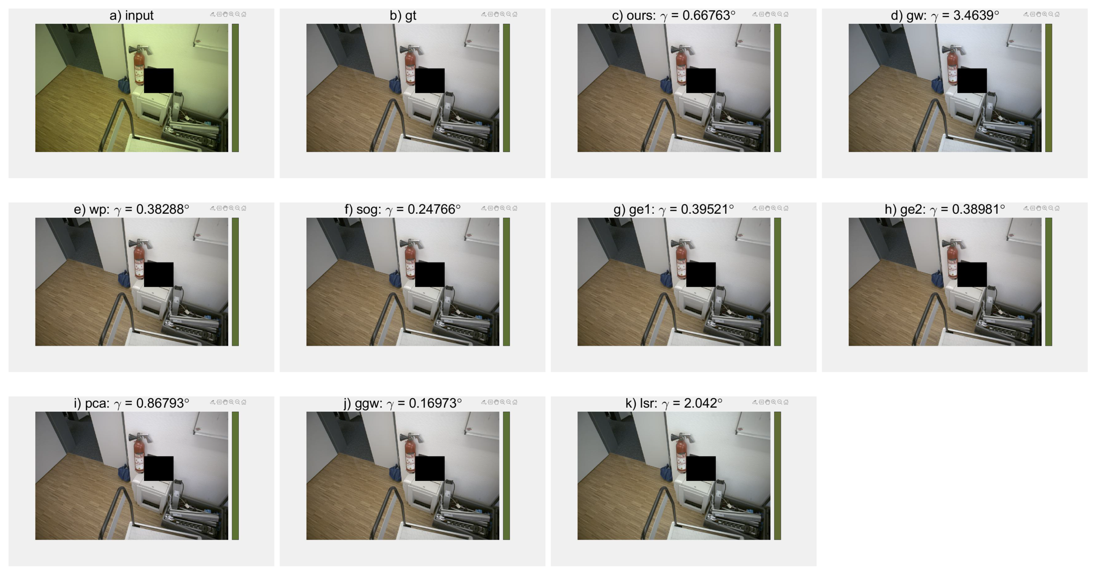
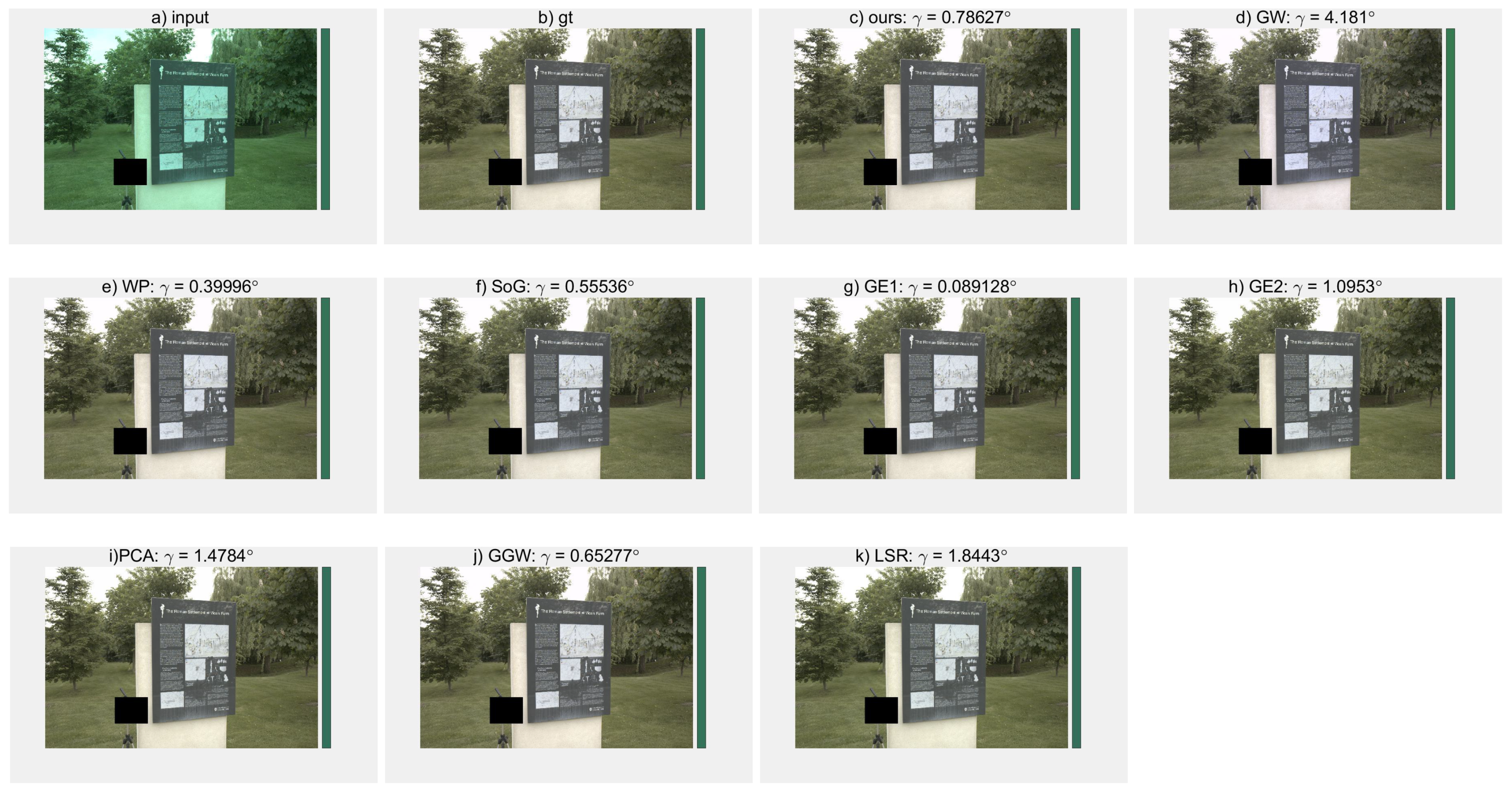
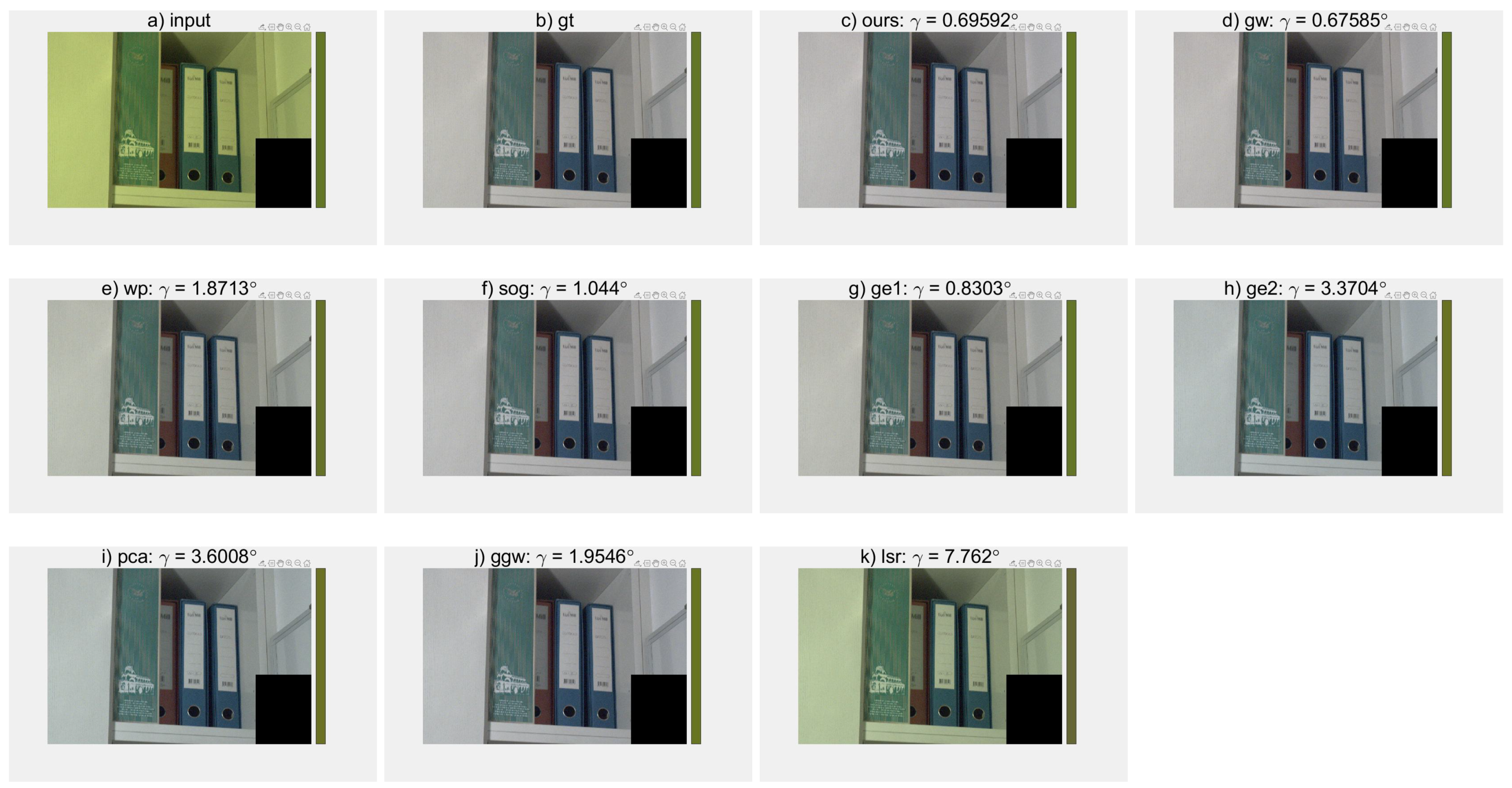
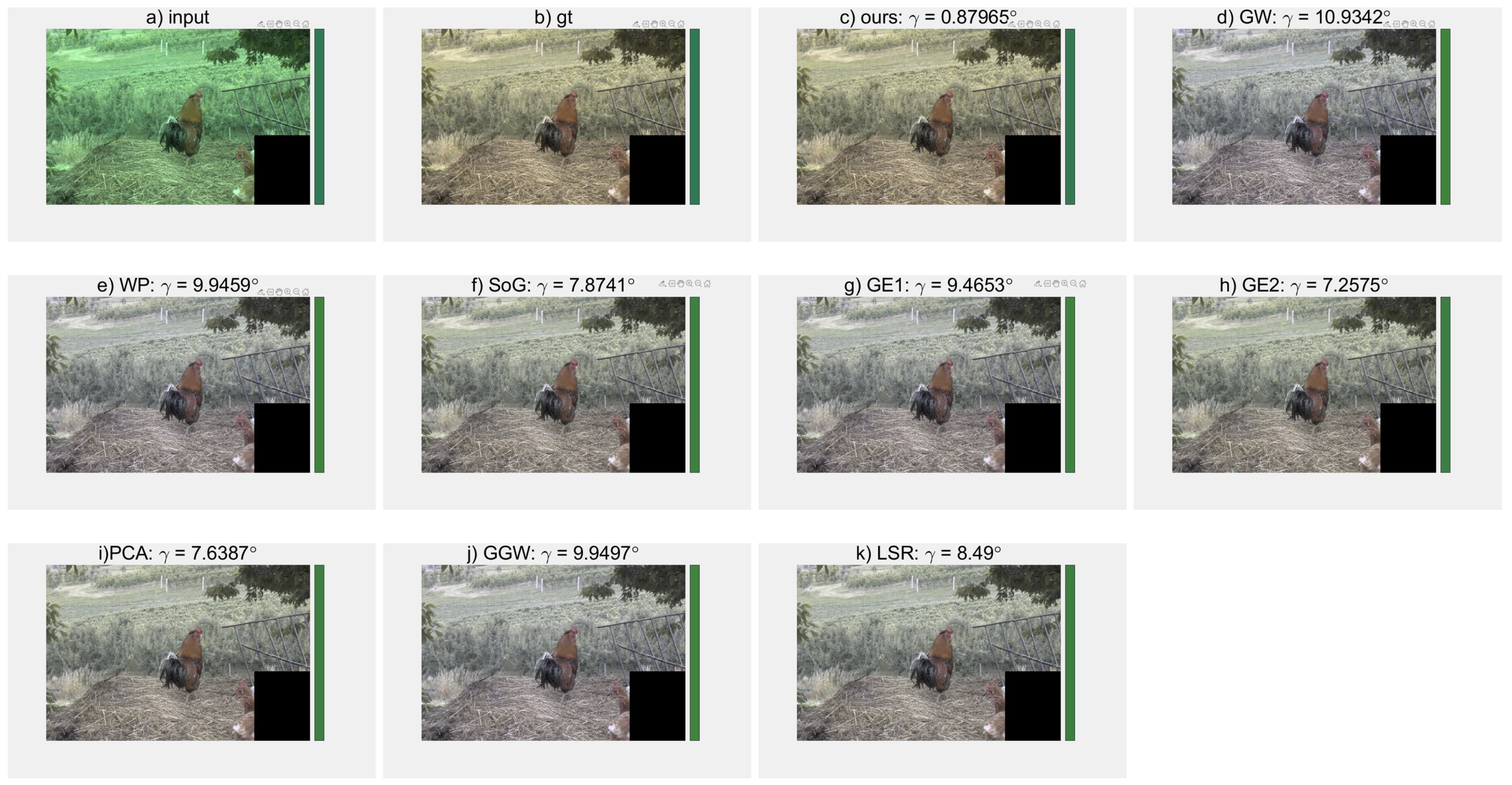
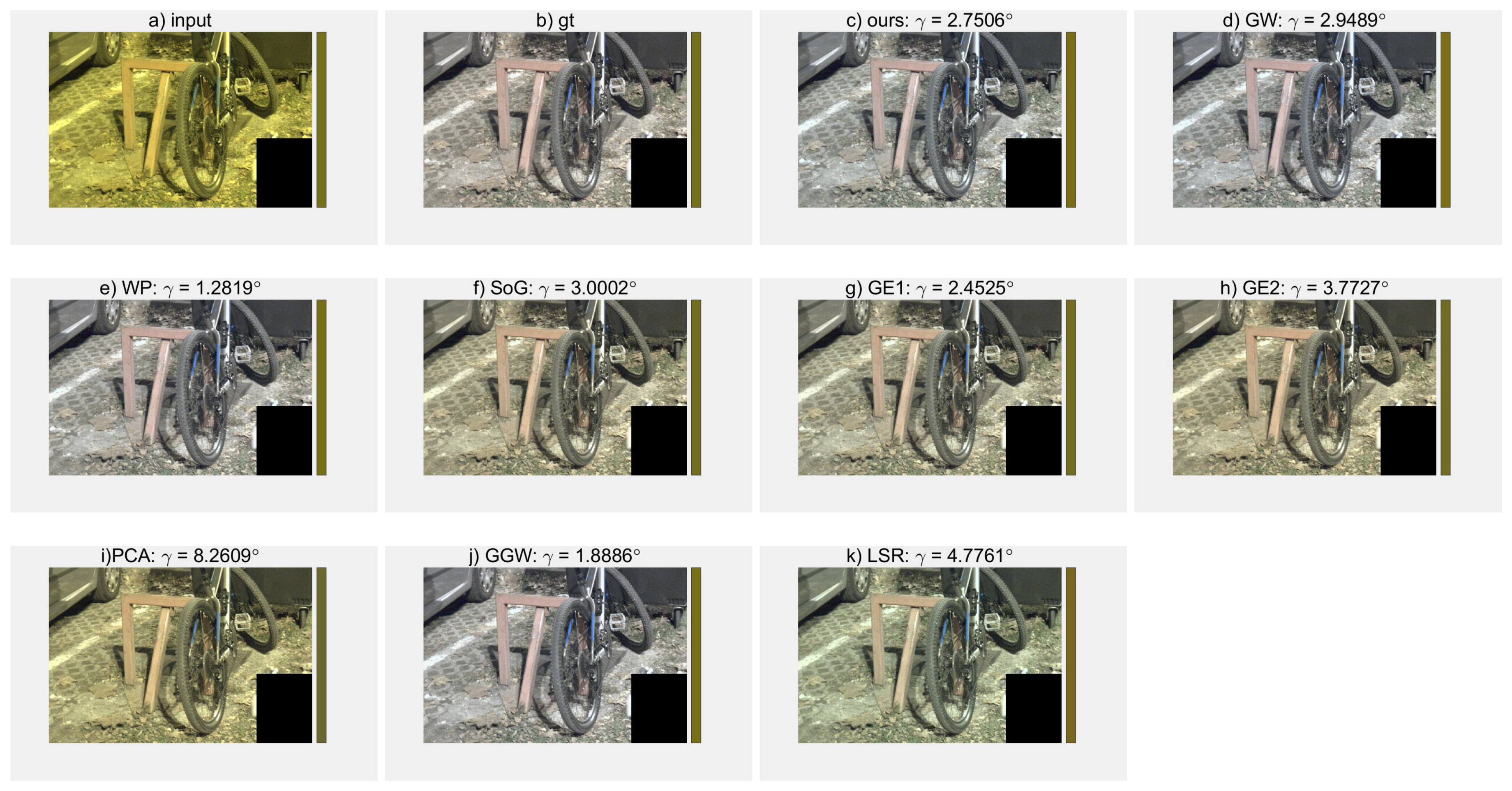
We provide some visual results for Gehler-Shi and Cube+ datasets, as shown in Figure 3, Figure 4, Figure 5, Figure 6 and Figure 7. For each input image, we show the ground truth, our estimated illuminant color and resulting white-balanced image, and other estimated illuminant colors and resulting white-balanced images using the unitary algorithms (GW, GGW, WP, GE1, GE2, SOG, PCA-based, and LSR). In these figures, the color bars on the right side of images (a) and (b) show the ground truth illuminant color. The color bar on the right side of images (c)–(k) shows the illuminant color estimated by the corresponding method, respectively. All images shown are rendered in sRGB color space.

In each one of Figure 3, Figure 4, Figure 5, Figure 6 and Figure 7, the AE between the estimated illuminant color and the ground truth is listed on the top of the resulting white-balanced image labelled from (c) to (k). It can be seen that for a given input image, the AE using our method has a value between the maximum and the minimum of all AEs using the unitary algorithms, and generally near the minimum. For example, in Figure 3, the AE using our method is 0.66, which is below the maxium of 3.46 for GW and near the minimum of 0.16 for GGW. Perhaps not surprisingly, since the proposed method is just based on a combination of unitary algorithms through ANFIS techniques, the result of the proposed method might not always be the best for a specific image. But from the view of entire dataset, the proposed method can obtain superior performances against other unitary algorithms. Results in Table 2 and Table 3 have already illustrated this observation.

4.4. Discussion and Further Analysis

We conduct many experiments to exploit the performance potentials of our proposed method. Besides cluster numbers, the factors influencing the performance of our proposal include different combination of unitary algorithms, sparsity of weight matrix obtained, etc.

Different cluster numbers. In this study, we performed two steps of image clustering, first CDF based, and then IIF based. Using k-means algorithm, the cluster number can be manually changed in order to obtain better clustering results. The bigger cluster number might make the trained model overfitting, but the smaller cluster number might make the trained model inaccurate due to its limited feature coverage. We used different values of $k_1$ and $k_2$ so as to find the appropriate choices for the two-step clustering.

Table 4. Statistical metrics on Gehler-Shi and Cube+ dataset with different cluster numbers (the lower, the better).

Cluster Numbers		Mean	Median	Trimean	Best 25%	Worst 25%
k1	k2
2	2	1.94	1.29	1.43	0.36	4.63
2	3	2.08	1.36	1.50	0.36	5.07
2	4	2.16	1.35	1.51	0.36	5.40
2	6	2.50	1.43	1.63	0.38	6.51
3	2	2.19	1.31	1.47	0.36	5.60
3	4	2.39	1.48	1.65	0.37	6.05
3	6	2.79	1.60	1.79	0.43	7.30
4	2	2.26	1.34	1.52	0.36	5.78
4	4	2.65	1.50	1.69	0.39	6.99
4	6	3.08	1.69	1.96	0.42	8.16
6	2	2.47	1.41	1.60	0.38	6.41
6	4	3.04	1.70	1.97	0.44	8.01

gives some statistics for the results using different values of $k_1$ and $k_2$. Through these tests, we found this two-step strategy is effective to group the training dataset, such that the images in the same cluster might have similar features that will be conducive to ANFIS modeling.

It should be noted that in Table 4, we limit $k_1·k_2$ into the range of $[4,24]$, as we find the settings with the total cluster number falling into this range will result in better estimation accuracy. We also can see from Table 4 that the two-step strategy with the choices of $k_1=2$ and $k_2=2$ produces the best estimation accuracy. Comparing the results using different $k_1$ and $k_2$, we find $k_1=2$ and $k_2=2$ are appropriate selections for our method on Gehler-Shi and Cube+ datasets. In our testing, we just have a combined dataset including 2275 images. Without doubt, if we use a larger image dataset, the number of $k_1{k}_2$ should increase for better modeling performances. To be a good case in point, k-means algorithm in paper [51] is used to cluster more than 20,000 images, where the cluster number is optimally set to be about 70.

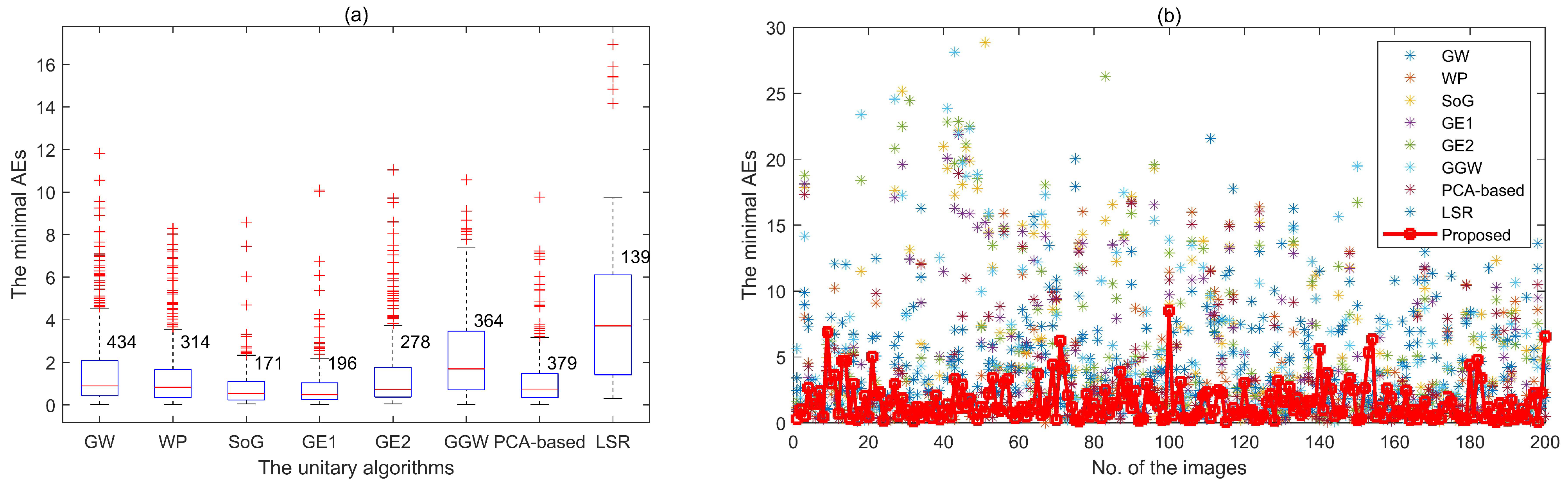
Different combination of unitary algorithms. By default, the proposed method uses the combination of eight unitary algorithms (GW, WP, SoG, GE1, GE2, GGW, PCA-based, and LSR), as we found for any image in our training dataset there are always some of these algorithms providing better illuminant estimation results. Figure 8a gives the distribution of the minimum AEs under these unitary algorithms for each image in Gehler-Shi and Cube+ datasets. It can be seen that for most images, there is a unitary algorithm to estimate illuminant color with AE being less than 3. This figure shows that if we use an appropriate, linear or nonlinear, combination of these unitary algorithms, it is possible to achieve better accuracy of illumnation estimation.

To further exploit better combination relationships, we design several combinations of these unitary algorithms to implement the proposed method. Some of them contain less than eight unitary algorithms. The experimental results are shown in

Table 5. Statistical metrics on Gehler-Shi and Cube+ datasets using different combination of unitary algorithms (the lower, the better).

Combinations of Unitary Algorithms	Mean	Median	Trimean	Best 25%	Worst 25%
GW, WP, SoG, GE1, GE2, GGW, PCA-based, LSR	2.20	1.46	1.60	0.40	5.31
GW, WP, SoG, GE1, GE2, GGW, PCA-based	2.32	1.50	1.67	0.45	5.62
GW, WP, SoG, GE1, GE2, GGW, LSR	2.21	1.47	1.62	0.40	5.33
GW, WP, SoG, GE1, GE2, GGW	2.27	1.50	1.68	0.44	5.44
GW, WP, SoG, GE1, PCA-based, LSR	2.07	1.36	1.50	0.39	5.00
GW, WP, SoG, GGW, PCA-based	2.20	1.42	1.58	0.38	5.39
GW, WP, SoG, GGW, LSR	2.12	1.38	1.53	0.39	5.16
GW, WP, SoG, GE1	2.19	1.43	1.60	0.41	5.29
GW, WP, GE2, GGW	2.15	1.46	1.62	0.42	5.12
Ours (GW, WP, PCA-based, LSR)	1.96	1.28	1.42	0.36	4.77

. The results indicate that the configuration with the combination of GW, WP, PCA-based, and LSR results in the best illuminant estimation accuracy. Figure 8b shows the minimum AE distribution for each method versus minimum AE obtainable with this chosen combination. It clearly shows the proposed method outperforms most of the eight unitary algorithms. It should be noted that this optimal combination might be just applicable for our experiments based on Gehler-Shi and Cube+ datasets. This experiment also indicates that seeking optimal combination is necessary to improve performances for illuminant estimation.

Using sparse weight matrix. In the proposed method, we use CDF weight vector $\eta$ and IIF weight matrix $\omega$ to measure what degree an image belongs to each cluster. We can define an integrated weight matrix $W=\left[w_{ij}\right],i=1,2,\cdots ,k_1,j=1,2,\cdots ,k_2$, where $w_{ij}={\eta }_i·{\omega }_{ij}$ is the final weight for the ij-th ANFIS predictor. Since commonly there are many elements in $\eta$ and $\omega$ much less than 1 and very near to zero, i.e., the weights or possibilities for an image belonging to some clusters are very low, we can set all these elements’ values to zero and then recalculate the values of other elements. For simplicity, we set a threshold $\epsilon$ for $w_{ij}$. If $w_{ij}<\epsilon$, set $w_{ij}=0$. W will become a sparse matrix $\overline{W}$. To assure the element summary of each row of $\overline{W}$ to be 1, recalculate $w_{ij}\ge \epsilon$, $i=1,2,\cdots ,k_1$, $j=1,2,\cdots ,k_2$, as below:

$${\overline{w}}_{ij}=\frac{w_{ij}}{\sum w_{i{j}^{*}}},$$

(28)

where $\sum w_{i{j}^{*}}$ represents the summary of all elements greater than $\epsilon$ in the i-th row of W.

We performed some experiments using the sparse weight matrix by setting $\epsilon$ between $[0.01,0.25]$. We find the results change towards slightly improvement along with the increasing value of $\epsilon$, and the best performance corresponds to $\epsilon =0.25$, as

Table 6. Statistical metrics on the Gehler-Shi and Cube+ datasets using sparse weight vector and matrix (the lower, the better).

Threshold Setting	Mean	Median	Trimean	Best 25%	Worst 25%
0.01	2.17	1.47	1.65	0.44	5.08
0.05	2.14	1.43	1.61	0.41	5.04
0.1	2.08	1.37	1.56	0.38	4.97
0.15	2.03	1.34	1.51	0.37	4.85
0.2	1.99	1.32	1.48	0.36	4.78
0.25	1.97	1.30	1.46	0.36	4.77

shows. By using the sparse weight matrix, we just need to weight a small number of outputs from ANFIS models, and the computation effort will reduce much more.

Comparison with one-step clustering. We also conduct experiments to validate the effectiveness of our proposed two-step clustering strategy against the one-step clustering method. In so-called one-step clustering, we keep $k_1$ or $k_2$ to be 1, and just change the value of the other one.

Table 7. Comparative statistical metrics on Gehler-Shi and Cube+ dataset with the one-step clustering and the proposed method (the lower, the better).

Cluster Numbers		Mean	Median	Trimean	Best 25%	Worst 25%
k1	k2
The one-step clustering
1	1	1.98	1.33	1.47	0.43	4.66
1	2	1.95	1.28	1.45	0.42	4.61
1	3	2.00	1.31	1.47	0.41	4.73
1	4	2.10	1.39	1.55	0.40	5.05
1	6	2.23	1.44	1.61	0.41	5.46
2	1	1.96	1.23	1.40	0.35	4.80
3	1	1.97	1.21	1.36	0.34	4.88
4	1	2.01	1.22	1.37	0.33	5.09
6	1	2.23	1.31	1.45	0.36	5.77
The proposed method
2	2	1.94	1.29	1.43	0.36	4.63

lists some statistical metrics for the results under different $k_1$ and $k_2$ values. In this table, Median and Trimean for $k_1=3$ and $k_2=1$, Best 25% for $k_1=4$ and $k_2=1$, and Worst 25% for $k_1=1$ and $k_2=2$ are all lower than the counterparts for $k_1=2$ and $k_2=2$. But the case with $k_1=2$ and $k_2=2$ has the lowest Mean and almost the best in the rest metrics. Moreover, we find that the values of Worst 25% will fluctuate with as much as 1.11 degrees for $k_2=1$. This implies that the illuminant estimation is not robust in this case. Therefore, we can say the proposed method using the two-step clustering with $k_1=2$ and $k_2=2$ is better than using the one-step strategy. We suppose that since CDFs and IIFs can be regarded as the representatives of different image characteristics, separately applying CDF and IIF to cluster the images, i.e., using two steps, may result in good performances.

5. Conclusions

In this study, we propose an ANFIS based approach to illuminant estimation. It allows illuminant estimation to be a fuzzy combination of multiple ANFIS predictions, in which underlying relationship between initial illumination estimates from some unitary algorithms and realistic illuminant color are accurately captured relying on the powerful learning and reasoning capability of ANFIS. Extensive experiments on the commonly used Gehler-Shi and Cube+ datasets demonstrate that our proposed method can obtain competing performances compared to many state-of-the-art approaches.

Although we found that some learning-based methods might outperform even the most carefully designed and tested combinations of statistical and fuzzy inference systems, the proposed method is good practice to apply ANFIS for illuminant estimation considering fuzzy inference in ANFIS eases to implement in imaging hardware with if-then rules and low computation efforts. In addition, one of the proposed method’s significant advantages is its extensibility to improve performances of illuminant estimation. When we have acquired additional benchmark images with available illumination ground truths, our provided framework can classify these incoming images and re-train the corresponding ANFIS models. Furthermore, we can exploit more effective feature clustering strategy, or seek optimal settings to train ANFIS models, after the training dataset is augmented with more samples. Our future research will focus on these avenues to further improve the performance of illuminant estimation.

References

1. Barnard, K.; Cardei, V.C.; Funt, B.V. A comparison of computational color constancy algorithms. I: Methodology and experiments with synthesized data. IEEE Trans. Image Process. 2002, 11, 972–984. [Google Scholar] [CrossRef]
2. Barnard, K.; Martin, L.; Coath, A.; Funt, B.V. A comparison of computational color constancy algorithms. II. Experiments with image data. IEEE Trans. Image Process. 2002, 11, 985–996. [Google Scholar] [CrossRef] [Green Version]
3. von Kries, J. Influence of adaptation on the effects produced by luminous stimuli. In Sources of Color Vision; MacAdam, D.L., Ed.; The MIT Press: Cambridge, MA, USA, 1970; pp. 109–119. [Google Scholar]
4. Buchsbaum, G. A spatial processor model for object colour perception. J. Frankl. Inst. 1980, 310, 1–26. [Google Scholar] [CrossRef]
5. Provenzi, E.; Gatta, C.; Fierro, M.; Rizzi, A. A spatially variant white-patch and gray-world method for color image enhancement driven by local contrast. IEEE Trans. Pattern Anal. Mach. Intell. 2008, 30, 1757–1770. [Google Scholar] [CrossRef]
6. Land, E.H. The retinex theory of color vision. Sci. Am. 1977, 237, 108–128. [Google Scholar] [CrossRef]
7. Finlayson, G.D.; Trezzi, E. Shades of gray and colour constancy. In Proceedings of the Twelfth Color Imaging Conference: Color Science and Engineering Systems, Technologies, Applications, CIC 2004, Scottsdale, AZ, USA, 9–12 November 2004; IS&T-The Society for Imaging Science and Technology: Fairfax County, VA, USA, 2004; pp. 37–41. [Google Scholar]
8. van de Weijer, J.; Gevers, T.; Gijsenij, A. Edge-based color constancy. IEEE Trans. Image Process. 2007, 16, 2207–2214. [Google Scholar] [CrossRef] [PubMed] [Green Version]
9. Gijsenij, A.; Gevers, T. Color constancy using natural image statistics and scene semantics. IEEE Trans. Pattern Anal. Mach. Intell. 2011, 33, 687–698. [Google Scholar] [CrossRef] [PubMed]
10. Bianco, S.; Ciocca, G.; Cusano, C.; Schettini, R. Automatic color constancy algorithm selection and combination. Pattern Recognit. 2010, 43, 695–705. [Google Scholar] [CrossRef]
11. Oh, S.W.; Kim, S.J. Approaching the computational color constancy as a classification problem through deep learning. Pattern Recognit. 2017, 61, 405–416. [Google Scholar] [CrossRef] [Green Version]
12. Hu, Y.; Wang, B.; Lin, S. FC4: Fully convolutional color constancy with confidence-weighted pooling. In Proceedings of the 2017 IEEE Conference on Computer Vision and Pattern Recognition, CVPR 2017, Honolulu, HI, USA, 21–26 July 2017; IEEE Computer Society: Piscataway, NJ, USA, 2017; pp. 330–339. [Google Scholar] [CrossRef]
13. Afifi, M.; Brown, M.S. Sensor-independent illumination estimation for DNN models. In Proceedings of the 30th British Machine Vision Conference 2019, BMVC 2019, Cardiff, UK, 9–12 September 2019; BMVA Press: London, UK, 2019; p. 282. [Google Scholar]
14. Afifi, M.; Brown, M.S. Deep white-balance editing. In Proceedings of the 2020 IEEE/CVF Conference on Computer Vision and Pattern Recognition, CVPR 2020, Seattle, WA, USA, 13–19 June 2020; Computer Vision Foundation/IEEE: Piscataway, NJ, USA, 2020; pp. 1394–1403. [Google Scholar] [CrossRef]
15. Koscevic, K.; Subasic, M.; Loncaric, S. Deep learning-based illumination estimation using light source classification. IEEE Access 2020, 8, 84239–84247. [Google Scholar] [CrossRef]
16. Xiao, J.; Gu, S.; Zhang, L. Multi-domain learning for accurate and few-shot color constancy. In Proceedings of the 2020 IEEE/CVF Conference on Computer Vision and Pattern Recognition, CVPR 2020, Seattle, WA, USA, 13–19 June 2020; Computer Vision Foundation/IEEE: Piscataway, NJ, USA, 2020; pp. 3255–3264. [Google Scholar] [CrossRef]
17. Hordley, S.D. Scene illuminant estimation: Past, present, and future. Color Res. Appl. 2006, 31, 303–314. [Google Scholar] [CrossRef]
18. Li, B.; Xiong, W.; Hu, W.; Funt, B.V. Evaluating combinational illumination estimation methods on real-world images. IEEE Trans. Image Process. 2014, 23, 1194–1209. [Google Scholar] [CrossRef] [PubMed]
19. Subhashdas, S.K.; Ha, Y.; Choi, D. Hybrid direct combination color constancy algorithm using ensemble of classifier. Expert Syst. Appl. 2019, 116, 410–429. [Google Scholar] [CrossRef]
20. Faghih, M.M.; Moghaddam, M.E. Multi-objective optimization based color constancy. Appl. Soft Comput. 2014, 17, 52–66. [Google Scholar] [CrossRef]
21. Banic, N.; Loncaric, S. Illumination estimation is sufficient for indoor-outdoor image classification. In Proceedings of the Pattern Recognition-40th German Conference, GCPR 2018, Stuttgart, Germany, 9–12 October 2018; Brox, T., Bruhn, A., Fritz, M., Eds.; Lecture Notes in Computer Science; Springer: Berlin/Heidelberg, Germany, 2018; Volume 11269, pp. 473–486. [Google Scholar] [CrossRef]
22. Koscevic, K.; Subasic, M.; Loncaric, S. Attention-based convolutional neural network for computer vision color constancy. In Proceedings of the 11th International Symposium on Image and Signal Processing and Analysis, ISPA 2019, Dubrovnik, Croatia, 23–25 September 2019; Loncaric, S., Bregovic, R., Carli, M., Subasic, M., Eds.; IEEE: Piscataway, NJ, USA, 2019; pp. 372–377. [Google Scholar] [CrossRef]
23. Gijsenij, A.; Gevers, T.; van de Weijer, J. Computational Color Constancy: Survey and Experiments. IEEE Trans. Image Process. 2011, 20, 2475–2489. [Google Scholar] [CrossRef]
24. Cepeda-Negrete, J.; Sánchez-Yáñez, R.E. Automatic selection of color constancy algorithms for dark image enhancement by fuzzy rule-based reasoning. Appl. Soft Comput. 2015, 28, 1–10. [Google Scholar] [CrossRef]
25. Cheng, D.; Prasad, D.K.; Brown, M.S. Illuminant estimation for color constancy: Why spatial-domain methods work and the role of the color distribution. J. Opt. Soc. Am. A 2014, 31, 1049. [Google Scholar] [CrossRef]
26. Gao, S.; Han, W.; Yang, K.; Li, C.; Li, Y. Efficient color constancy with local surface reflectance statistics. In Proceedings of the Computer Vision-ECCV 2014-13th European Conference, Zurich, Switzerland, 6–12 September 2014; Proceedings, Part II. Fleet, D.J., Pajdla, T., Schiele, B., Tuytelaars, T., Eds.; Lecture Notes in Computer Science. Springer: Berlin/Heidelberg, Germany, 2014; Volume 8690, pp. 158–173. [Google Scholar] [CrossRef]
27. Bianco, S.; Gasparini, F.; Schettini, R. Consensus-based framework for illuminant chromaticity estimation. J. Electron. Imaging 2008, 17, 023013. [Google Scholar] [CrossRef] [Green Version]
28. Lu, R.; Gijsenij, A.; Gevers, T.; Nedovic, V.; Xu, D.; Geusebroek, J. Color constancy using 3D scene geometry. In Proceedings of the IEEE 12th International Conference on Computer Vision, ICCV 2009, Kyoto, Japan, 27 September–4 October 2009; IEEE Computer Society: Piscataway, NJ, USA, 2009; pp. 1749–1756. [Google Scholar] [CrossRef] [Green Version]
29. Nedovic, V.; Smeulders, A.W.M.; Redert, A.; Geusebroek, J. Stages as models of scene geometry. IEEE Trans. Pattern Anal. Mach. Intell. 2010, 32, 1673–1687. [Google Scholar] [CrossRef] [Green Version]
30. Huang, X.; Li, B.; Li, S.; Li, W.; Xiong, W.; Yin, X.; Hu, W.; Qin, H. Multi-cue semi-supervised color constancy with limited training samples. IEEE Trans. Image Process. 2020, 29, 7875–7888. [Google Scholar] [CrossRef]
31. van de Weijer, J.; Schmid, C.; Verbeek, J.J. Using high-level visual information for color constancy. In Proceedings of the IEEE 11th International Conference on Computer Vision, ICCV 2007, Rio de Janeiro, Brazil, 14–20 October 2007; IEEE Computer Society: Piscataway, NJ, USA, 2007; pp. 1–8. [Google Scholar] [CrossRef] [Green Version]
32. Li, B.; Xiong, W.; Xu, D.; Bao, H. A supervised combination strategy for illumination chromaticity estimation. ACM Trans. Appl. Percept. 2010, 8, 5:1–5:17. [Google Scholar] [CrossRef]
33. Cardei, V.C.; Funt, B.V. Committee-based color constancy. In Proceedings of the Seventh Color Imaging Conference: Color Science, Systems, and Applications Putting It All Together, CIC 1999, Scottsdale, AZ, USA, 16–19 November 1999; IS&T-The Society for Imaging Science and Technology: Fairfax County, VA, USA, 1999; pp. 311–313. [Google Scholar]
34. Wang, C.; Zhu, Z.; Chen, S.; Yang, J. Illumination correction via support vector regression based on improved whale optimization algorithm. Color Res. Appl. 2021, 46, 303–318. [Google Scholar] [CrossRef]
35. Cheng, D.; Price, B.L.; Cohen, S.; Brown, M.S. Effective learning-based illuminant estimation using simple features. In Proceedings of the IEEE Conference on Computer Vision and Pattern Recognition, CVPR 2015, Boston, MA, USA, 7–12 June 2015; IEEE Computer Society: Piscataway, NJ, USA, 2015; pp. 1000–1008. [Google Scholar] [CrossRef]
36. Lau, C.K.; Ghosh, K.; Hussain, M.A.; Che Hassan, C.R. Fault diagnosis of Tennessee Eastman process with multi-scale PCA and ANFIS. Chemom. Intell. Lab. Syst. 2013, 120, 1–14. [Google Scholar] [CrossRef]
37. Seyyedattar, M.; Ghiasi, M.M.; Zendehboudi, S.; Butt, S. Determination of bubble point pressure and oil formation volume factor: Extra trees compared with LSSVM-CSA hybrid and ANFIS models. Fuel 2020, 269, 1–18. [Google Scholar] [CrossRef]
38. Hemrit, G.; Finlayson, G.D.; Gijsenij, A.; Gehler, P.; Bianco, S.; Drew, M.S.; Funt, B.; Shi, L. Providing a single ground-truth for illuminant estimation for the ColorChecker dataset. IEEE Trans. Pattern Anal. Mach. Intell. 2020, 42, 1286–1287. [Google Scholar] [CrossRef] [Green Version]
39. Banic, N.; Loncaric, S. Unsupervised learning for color constancy. In Proceedings of the 13th International Joint Conference on Computer Vision, Imaging and Computer Graphics Theory and Applications (VISIGRAPP 2018)-Volume 4: VISAPP, Funchal, Madeira, Portugal, 27–29 January 2018; Trémeau, A., Imai, F.H., Braz, J., Eds.; SciTePress: Setúbal, Portugal, 2018; pp. 181–188. [Google Scholar] [CrossRef]
40. Hussain, M.A.; Akbari, A.S.; Halpin, E.A. Color constancy for uniform and non-uniform illuminant using image texture. IEEE Access 2019, 7, 72964–72978. [Google Scholar] [CrossRef]
41. Joze, H.R.V.; Drew, M.S. Exemplar-based color constancy and multiple illumination. IEEE Trans. Pattern Anal. Mach. Intell. 2014, 36, 860–873. [Google Scholar] [CrossRef] [PubMed]
42. Bianco, S.; Cusano, C.; Schettini, R. Color constancy using CNNs. In Proceedings of the 2015 IEEE Conference on Computer Vision and Pattern Recognition Workshops, CVPR Workshops 2015, Boston, MA, USA, 7–12 June 2015; IEEE Computer Society: Piscataway, NJ, USA, 2015; pp. 81–89. [Google Scholar] [CrossRef] [Green Version]
43. Choi, H.H.; Kang, H.S.; Yun, B.J. CNN-based illumination estimation with semantic information. Appl. Sci. 2020, 10, 4806. [Google Scholar] [CrossRef]
44. Qiu, J.; Xu, H.; Ye, Z. Color constancy by reweighting image feature maps. IEEE Trans. Image Process. 2020, 29, 5711–5721. [Google Scholar] [CrossRef] [PubMed] [Green Version]
45. Gijsenij, A.; Gevers, T.; van de Weijer, J. Generalized gamut mapping using image derivative structures for color constancy. Int. J. Comput. Vis. 2010, 86, 127–139. [Google Scholar] [CrossRef] [Green Version]
46. Gehler, P.V.; Rother, C.; Blake, A.; Minka, T.P.; Sharp, T. Bayesian color constancy revisited. In Proceedings of the 2008 IEEE Computer Society Conference on Computer Vision and Pattern Recognition (CVPR 2008), Anchorage, AK, USA, 24–26 June 2008; IEEE Computer Society: Piscataway, NJ, USA, 2008. [Google Scholar] [CrossRef]
47. Shi, W.; Loy, C.C.; Tang, X. Deep specialized network for illuminant estimation. In Proceedings of the Computer Vision-ECCV 2016-14th European Conference, Amsterdam, The Netherlands, 11–14 October 2016; Proceedings, Part IV. Leibe, B., Matas, J., Sebe, N., Welling, M., Eds.; Lecture Notes in Computer Science. Springer: Berlin/Heidelberg, Germany, 2016; Volume 9908, pp. 371–387. [Google Scholar] [CrossRef]
48. Koscevic, K.; Banic, N.; Loncaric, S. Color beaver: Bounding illumination estimations for higher accuracy. In Proceedings of the 14th International Joint Conference on Computer Vision, Imaging and Computer Graphics Theory and Applications, VISIGRAPP 2019, Volume 4: VISAPP, Prague, Czech Republic, 25–27 February 2019; Trémeau, A., Farinella, G.M., Braz, J., Eds.; SciTePress: Setúbal, Portugal, 2019; pp. 183–190. [Google Scholar] [CrossRef]
49. Yang, K.; Gao, S.; Li, Y. Efficient illuminant estimation for color constancy using grey pixels. In Proceedings of the IEEE Conference on Computer Vision and Pattern Recognition, CVPR 2015, Boston, MA, USA, 7–12 June 2015; IEEE Computer Society: Piscataway, NJ, USA, 2015; pp. 2254–2263. [Google Scholar] [CrossRef]
50. Koscevic, K.; Subasic, M.; Loncaric, S. Guiding the illumination estimation using the attention mechanism. In Proceedings of the 2020 2nd Asia Pacific Information Technology Conference, APIT 2020, Bali Island, Indonesia, 17–19 January 2020; Association for Computing Machinery: New York, NY, USA, 2020; pp. 143–149. [Google Scholar] [CrossRef] [Green Version]
51. Afifi, M.; Brown, M.S. Interactive white balancing for camera-rendered images. CoRR 2020, 2020, 136–141. [Google Scholar] [CrossRef]
Figure 1. Overview of the training phase and the testing phase for the proposed approach.
Applsci 11 09936 g001
Figure 2. Examples of membership functions used by the ANFIS models developed for (a) estimation of r component, (b) estimation of g component, and (c) estimation of b component. In these three models, the inputs are chromaticity values of r i and g i ( i = 1 , 2 , 3 , 4 ) from the unitary algorithms: GW, WP, PCA-based, and LSR, respectively. The curves in cyan, purple, yellow, and magenta indicate the membership values for the four cluster regions respectively, responding to the number of clusters to be 4.
Applsci 11 09936 g002
Figure 3. Example results for indoor scene from the Gehler-Shi dataset: (a) input image; (b) ground truth; (c) ours; (d) GW; (e) GGW; (f) WP; (g) GE1; (h) GE2; (i) SOG; (j) PCA-based; and (k) LSR, respectively. All images shown are rendered in sRGB color space.
Applsci 11 09936 g003
Figure 4. Example results for natural lighting scene taken from the Gehler-Shi dataset: (a) input image; (b) ground truth; (c) ours; (d) GW; (e) GGW; (f) WP; (g) GE1; (h) GE2; (i) SOG; (j) PCA-based; and (k) LSR, respectively. All images shown are rendered in sRGB color space.
Applsci 11 09936 g004
Figure 5. Example results for indoor scene taken from the Cube+ dataset: (a) input image; (b) ground truth; (c) ours; (d) GW; (e) GGW; (f) WP; (g) GE1; (h) GE2; (i) SOG; (j) PCA-based; and (k) LSR, respectively. All images shown are rendered in sRGB color space.
Applsci 11 09936 g005
Figure 6. Example results for outdoor natural lighting scene taken from the Cube+ dataset: (a) input image; (b) ground truth; (c) ours; (d) GW; (e) GGW; (f) WP; (g) GE1; (h) GE2; (i) SOG; (j) PCA-based; and (k) LSR, respectively. All images shown are rendered in sRGB color space.
Applsci 11 09936 g006
Figure 7. Example results for outdoor artificial lighting scene taken from the Cube+ dataset: (a) input image; (b) ground truth; (c) ours; (d) GW; (e) GGW; (f) WP; (g) GE1; (h) GE2; (i) SOG; (j) PCA-based; and (k) LSR, respectively. All images shown are rendered in sRGB color space.
Applsci 11 09936 g007
Figure 8. Boxplot and plot of minimum AEs’ distribution: (a) the distribution of the minimum AE across the 8 methods, and (b) the minimum AE distribution for each method versus minimum AE obtainable with chosen combination of methods. The value near the box of each unitary algorithm indicates the number of the corresponding algorithm with minimum AE across the 8 methods. It can be seen from the left subfigure that for most images there is at least one unitary algorithm to estimate its illuminant color resulting in AE no more than 3. This right subfigure shows the minimum AEs of the proposed method with the chosen combination outperforms most of the eight unitary algorithms, where No. of images 1~100 are the first 100 images in the Gehler-Shi dataset, and No. of images 101~200 the first 100 images in the Cube+ dataset. Due to limited length, we just show the results for 200 images.
Applsci 11 09936 g008