Air-Water Bubbly Flow by Multiple Vents on a Hydrofoil in a Steady Free-Stream

Abstract

Flow features, due to air injection through multiple vents on the surface of a hydrofoil inclined at an angle with respect to the free-stream in a cavitation tunnel, are presented here. The hydrofoil, with a chord length, c, is oriented at the angle of inclination, $\alpha$ = 3.5°. The Froude number, $Fn$, based on the free-stream velocity, $V_{\infty }$, and air injection vent diameter, $d_h$, is 30.30, 50.51 and 70.71. Air is injected through multiple vents on the hydrofoil at the non-dimensional air injection coefficient, $C_q\sim 16-8917$. The air bubble packing per unit area is quantified using spatial density, $S_D$, at various combinations of $Fn,C_q$ based on a high-speed video from the side view. The time-averaged spatial density, $<S_D>$, is observed to increase in a logarithmic manner with an increase in the air injection rate, Q, at various Froude numbers. There is an increase in the mean spatial density of the bubbles with the increase in $C_q$ at all $Fn$. A power–law relation is shown to exist between the time-averaged spatial density, $<S_D>$, and the non-dimensional flow variables, Reynolds number, ${Re}_{air}$, $Fn$ and $C_q$ based on a regression analysis. By tracking individual finite volume bubbles flowing with the free-stream, the bubble dimensions in pixels are quantified using quantities such as the deformation rate, $ϵ$, and standardization, ${ϵ}_S$, from the side-view videos. It is observed that $ϵ$ and ${ϵ}_S$ change with time, even as they become advected with the free-stream. Through high-speed imaging from the top view, we characterize the bubbly flow features’ time-averaged thickness, t, at various combinations of $Fn,C_q$ at $\alpha$ = 3.5°. We obtain a power-law relation between the non-dimensional time-averaged jet thickness, $t/c$, and the non-dimensional flow parameters such as, ${Re}_{air}$, $Fn,C_q$ and the non-dimensional streamwise distance, $x/x_{ref}$, based on a regression analysis, where $x_{ref}$ is a reference distance. The results are relevant to engineering applications where the air–water bubbly flow in a free-stream is important.

1. Introduction

The two-phase flow of air injection in water in engineering applications affects drag reduction and noise attenuation benefits. Elbing [1] performed drag measurements using skin-friction force balances on the surface of a flat plate in a cavitation tunnel and found a linear increase in the drag reduction percentage with the increase in the air injection coefficient. Yanuar [2] measured the total drag coefficient exerted on a model ship in a towing tank using a load cell transducer with air injection underneath the surface in two different air injection configurations. They demonstrated a decrease in the total drag coefficient upon air injection for the two configurations, when compared against the no-injection case at several Froude numbers. The hydrodynamic performance of the National Advisory Committee for Aeronautics (NACA) 4412 hydrofoil in the free-stream flow of two-phase air and water was studied by Ohasi [3]. The air–water void fraction distribution in the wall-normal direction around a hydrofoil was quantified at several streamwise distances from the leading edge at a known angle of inclination and free-stream velocity. Ayers [4] used an air bubble curtain to reduce the noise emitted from seismic exploration vehicles. They measured a considerable sound transmission loss across the measured sound frequency range at several sound incident angles on the sound curtain. Air bubbles, generated due to the flow past a 2D cylinder in the vicinity of the free surface at different angles of inclination about the horizontal, were studied at various free-stream velocities by Kumagi [5]. They introduced the winged-air induction pipe (WAIP) that generates bubbles to affect drag reduction in ships. Kumagi [6] further utilized WAIP to affect the drag reduction in a ship and noted a marked reduction in fuel consumption across the ship speed upon the usage of WAIP. They also noted a marked decrease in fuel consumption per day with an increase in the number of WAIPs installed on the hull surface. Amromin [7] performed a force balance measurement of a towed model ship and demonstrated a drag reduction on a model with air injection in the hull region. Wu [8] injected air under the surface of a model ship hull in a towing tank facility and found a drag reduction due to air injection by force measurements. Jang [9] measured the drag force exerted on a flat plate and found considerable drag-reduction benefits due to air injection, when compared without air injection. Mohanarangam [10] performed numerical simulations of a micro-bubble drag reduction on a flat plate using a two-fluid model. They showed an upward shift in the non-dimensional velocity, $u^{+}$, in the non-dimensional wall-normal coordinate, $y^{+}$ due to air injection, which is conducive for drag-reduction applications. Mizokami [11] demonstrated a reduction in horse-power required to drive a model hull with an increase in the air layer thickness at several hull speeds. Murai [12] utilized the NACA 0012 hydrofoil and NACA 4412 hydrofoil as bubble generators on a model ship. The potential drag reduction benefit was demonstrated by them with a marked increase in the number of bubbles in the observation field with an increase in the velocity of the towed ship model from high-speed imaging. Makiharju [13] estimated net energy savings due to the drag reduction upon air injection underneath a conventional ship.

The bubbles ensuing from two different hydrofoils at various angles of inclination, free-stream velocities and air injection rates were characterized by a shadow imaging technique in the work of Karn [14]. They quantified the bubble diameter distribution at several combinations of non-dimensional flow parameters. Han [15] studied the bubble size distribution around a NACA 0015 hydrofoil using a two-fluid mathematical model in a two-phase flow. The optimal range of bubble size at various free-stream velocities which result in drag reduction was identified by Murai [16]. The roll of bubbles in the dynamics of a cavitating hydrofoil and the vortices shed behind them were highlighted by large eddy simulations by Yu [17]. The dynamics of three-dimensional air bubbles are studied by two-dimensional imaging of the bubbles in the current work, as was performed in the works of Wang [18], Ying [19], Cheng [20]. The dynamics of raising air bubbles in water and polyglycol were studies by high speed imaging in the experiments of Acuna [21]. Oishi [22] studied the dynamics of injected air bubbles in a horizontal channel at several Reynolds numbers by high-speed imaging and, also, measured a considerable reduction in the frictional coefficient owing to air injection at large Reynolds numbers. Although several studies have shown drag reduction benefits and noise attenuation due to air injection, studies that characterize the bubble size, bubble density and bubble dynamics upon air injection in water are quite limited. The novelty of the current work is in characterizing the bubbles observed upon air injection from an array of air vents on the surface of an inclined hydrofoil in a steady free-stream by high-speed imaging. We describe the temporal variation of the bubble size, number of bubbles per unit area as observed from the side view and the thickness of the air jet as observed from the top view.

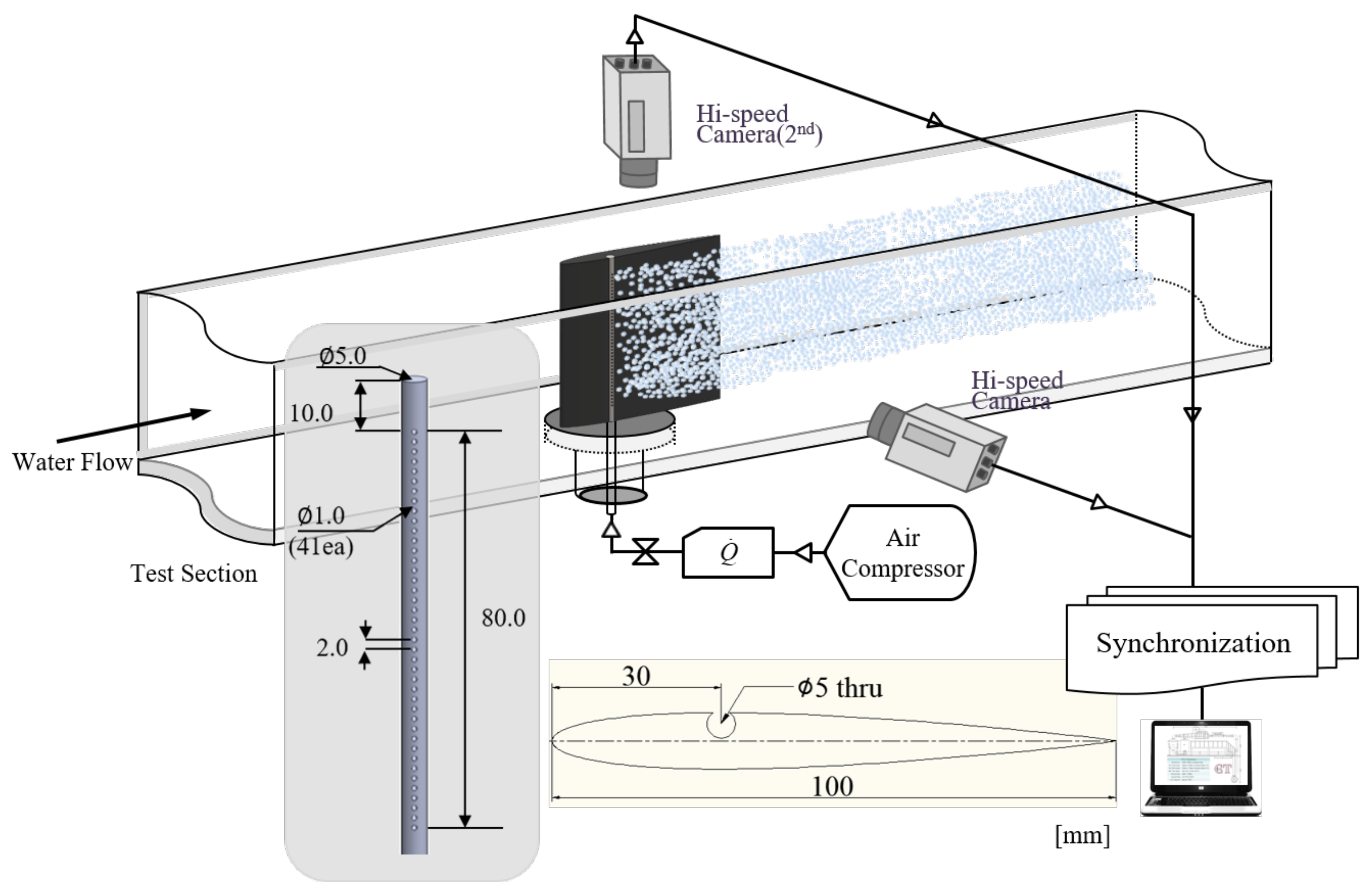
2. Experimental Method

The experiments on air injection through multiple vents on an inclined NACA 0010 hydrofoil in a steady free-stream were performed in Chungnam National University Cavitation Tunnel (CNU-CT), and it was geometrically analogous to the air injection through the hull surface of a ship [1]. The NACA 0010 hydrofoil hd a chord length of 100 mm and had a maximum thickness of 10 mm. The test section of the cavitation tunnel was 100 mm in width and 100 mm in breadth and it was 1.4 m long. The contraction ratio of the converging section ahead of the test section was 5:1. The pressure within the tunnel could vary from 0.1 bar to 3 bar. The maximum attainable tunnel velocity was 20 m/s. There were provisions for the removal of air bubbles suspended in water ahead of the test section. The drawing of the cavitation tunnel is given in Nagarathinam [23]. The current experimental setup consisted of a hydrofoil placed in the test section of CNU-CT in a steady free-stream flow at the angle of inclination of $\alpha$ = 3.5°. Air was injected through an array of vent holes on the hydrofoil surface. The air injection vents of 1 mm diameter were arrayed at $x/c$ = 0.3, which was the point of maximum thickness for NACA 0010 hydrofoil. The schematic of the experimental setup used in the current experiments is shown in Figure 1. The hydrofoil with multiple air vents placed in a uniform stream at the angle of inclination of 3.5° was shown in the schematic. The flow was imaged using high-speed cameras and the air injection rate was metered through a calibrated air injection pump, having an accuracy of ±0.8% at the calibration conditions, in terms of Standard Liter Per Minute (SLPM). The high-speed cameras were capable of imaging the flow field at the rate of 8000 frames per second, at the resolution of 1920 × 1080 pixels on a CMOS sensor. The minimum shutter speed of the camera was 3.9 μs. The control variables in the present problem were air injection rate, Q, free-stream velocity, $V_{\infty }$, with angle of inclination of the hydrofoil, $\alpha$, held constant at 3.5° and the tunnel ambient pressure was held constant at 1 bar. The non-dimensional air injection rate was defined as $C_q=V_{\infty }{c}^2/Q$ and the Froude number, $Fn$, was defined as $Fn=V_{\infty }/\sqrt{g{d}_v}$, where $d_v$ was the air injection vent diameter; Reynolds number was defined as $R{e}_{air}={\rho }_{air}{V}_{inj}c/{\mu }_{air}$, where ${\rho }_{air}$ was the density of air, ${\mu }_{air}$ was the viscosity of air, injection velocity, $V_{inj}=Q/dn{d}_v$, where d was the thickness of the hydrofoil; n was the number of injection vents, which was equal to forty-one in the current experiments.

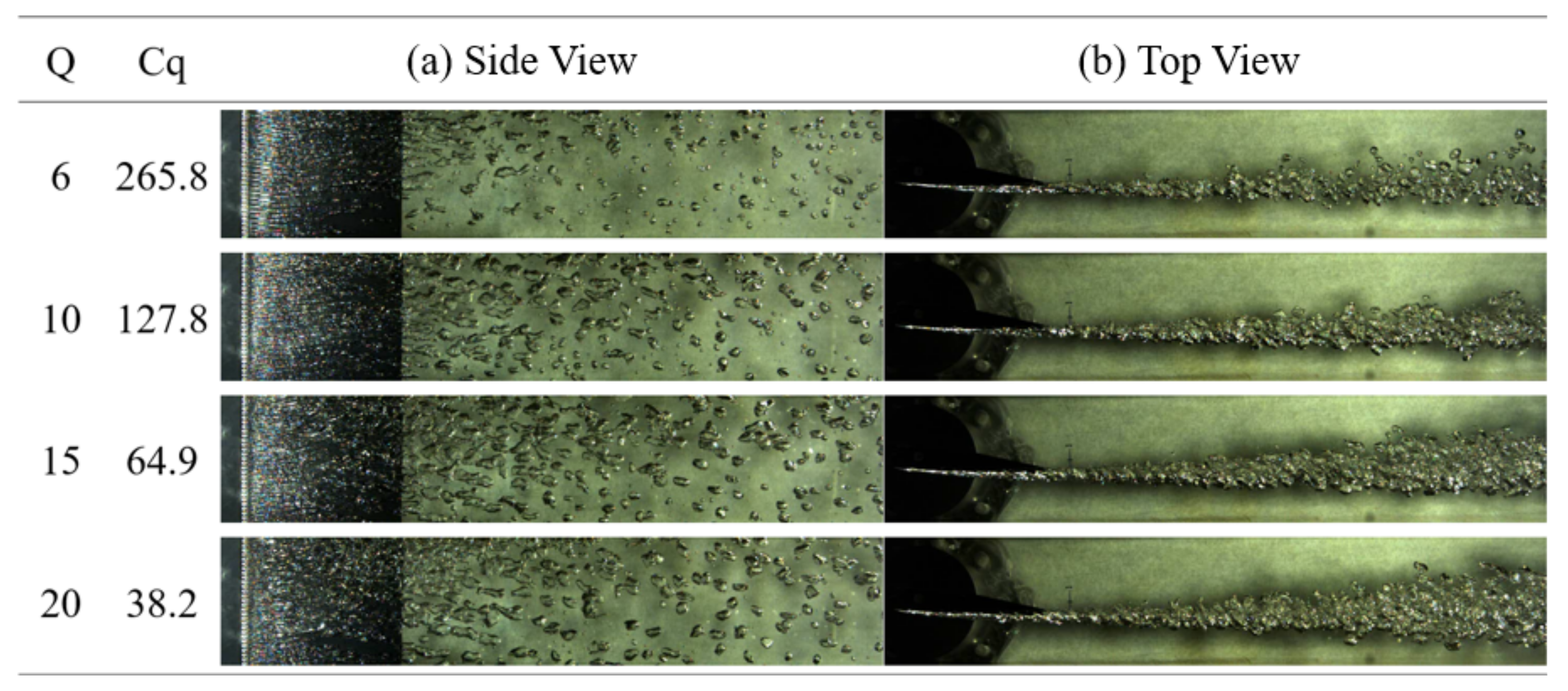
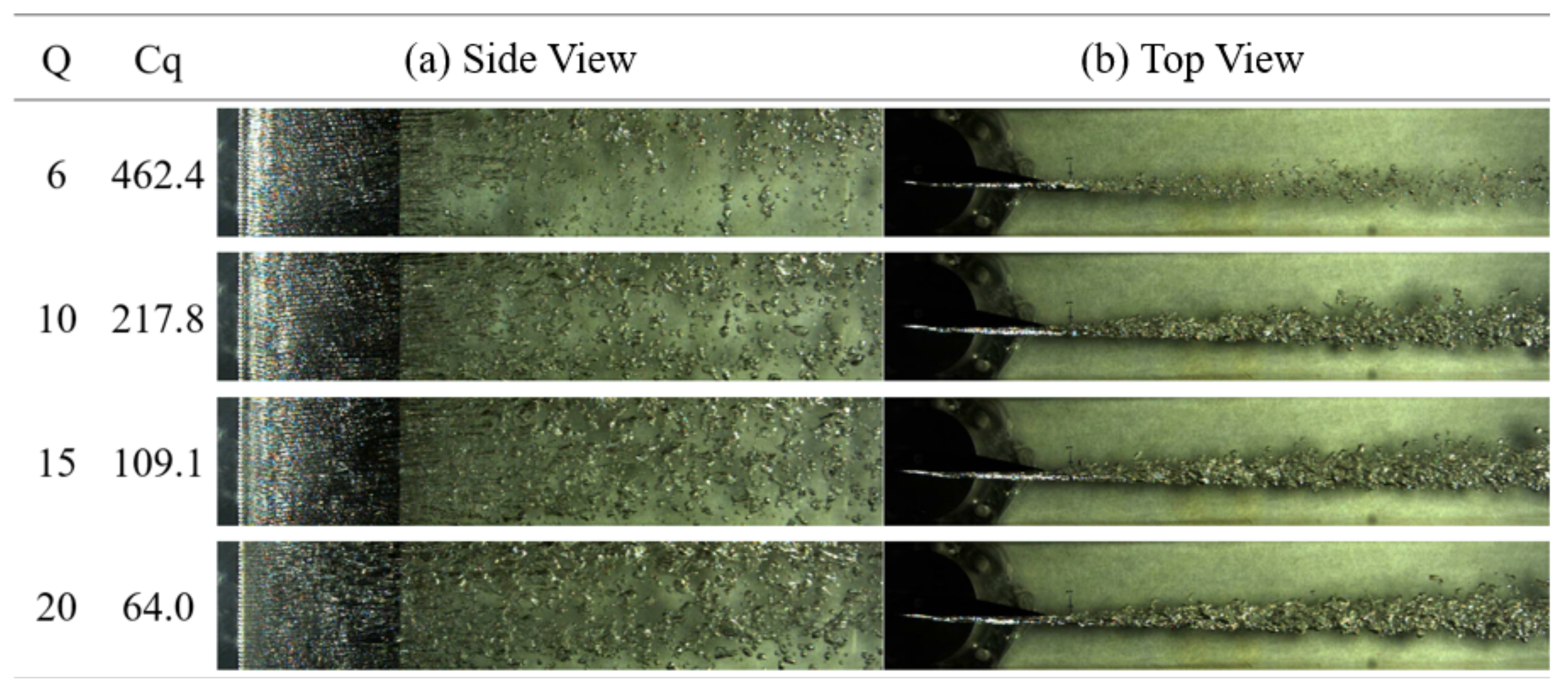
3. Results and Discussion

Experiments were performed with a view to characterize the bubbles issuing through multiple vents on the inclined hydrofoil at various air injection rates and free-stream velocities. The air jet properties of interest were the bubble size, number of bubbles per unit area as observed from the side view and the time-averaged jet thickness, t, as observed from the top view under various $Fn$, $C_q$ combinations at $\alpha$ = 3.5°. The jet thickness, t, referred to in the paper was the time-averaged quantity, which was defined as the ratio of the sum of the jet thickness observed at each individual frame to the total number of frames. The bubbles, due to air injection through multiple vents on the hydrofoil surface at the Froude number of 30.3 for various $C_q$ values, are shown in Figure 2 (multimedia view). It was observed that the air injected through the forty-one vent holes on the hydrofoil surface broke down into small bubbles and were advected downstream along the free-stream. Shown in Figure 2 (multimedia view) are the instantaneous side view and top view observations for $C_q=265-38$ at $Fn=30.3$. It was observed visually from the figure that there was an increase in the number of bubbles with an increase in the air injection rate at a given Froude number by comparing the frames in the side-view column in Figure 2 (multimedia view). It may also be stated qualitatively that there was an increase in the jet thickness with the increase in Q at large downstream distances as observed from the frames in the top-view column of Figure 2 (multimedia view).

Instantaneous frames showing the air bubbles, due to air injection through multiple vents on the surface of the hydrofoil at $Fn=50.5,70.7$, are shown in Figure 3 (multimedia view) and Figure 4 (multimedia view), respectively. At a given Q, the bubble size appeared to have become smaller with the increase in the free-stream velocity by comparing the frames in the side-view columns of Figure 2 (multimedia view) with the corresponding frames in the side-view columns in Figure 3 (multimedia view) and Figure 4 (multimedia view). The bubble size reduction at a given air injection coefficient with the increase in the free-stream velocity was analogous to the findings of Walton [24], who quantified the droplet size for the spray issuing through an impaction spray nozzle at various free-stream velocities. As observed in Figure 3 (multimedia view) and Figure 4 (multimedia view), with the increase in the free-stream velocity, there was an increase in the number of bubbles, qualitatively, in a unit area at a given air injection rate, Q. Similar to Figure 2 (multimedia view), through a visual observation of the top-view frames for both $Fn=50.5,70.7$ in Figure 3 (multimedia view) and Figure 4 (multimedia view), it can be stated that there was an increase in the jet thickness at large downstream distances with the increase in the air injection rate at a given free-stream velocity.

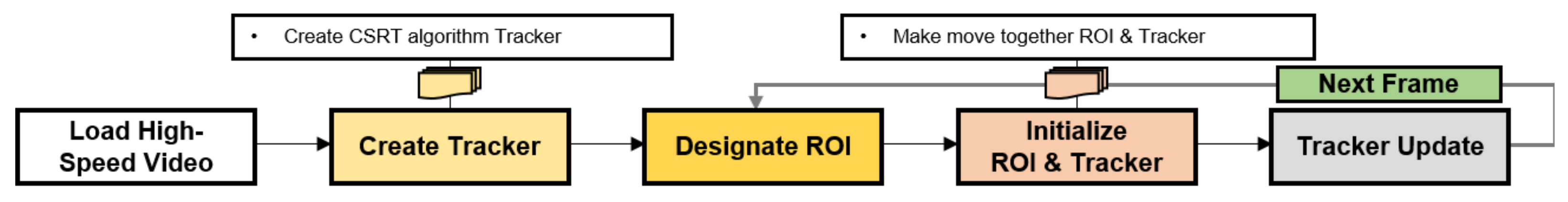
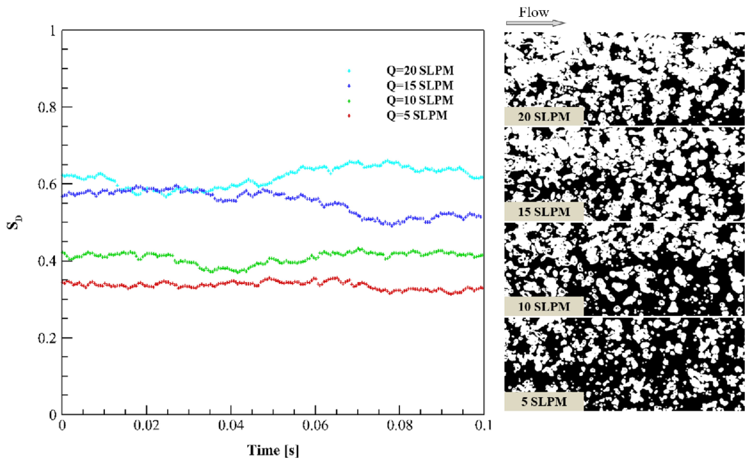
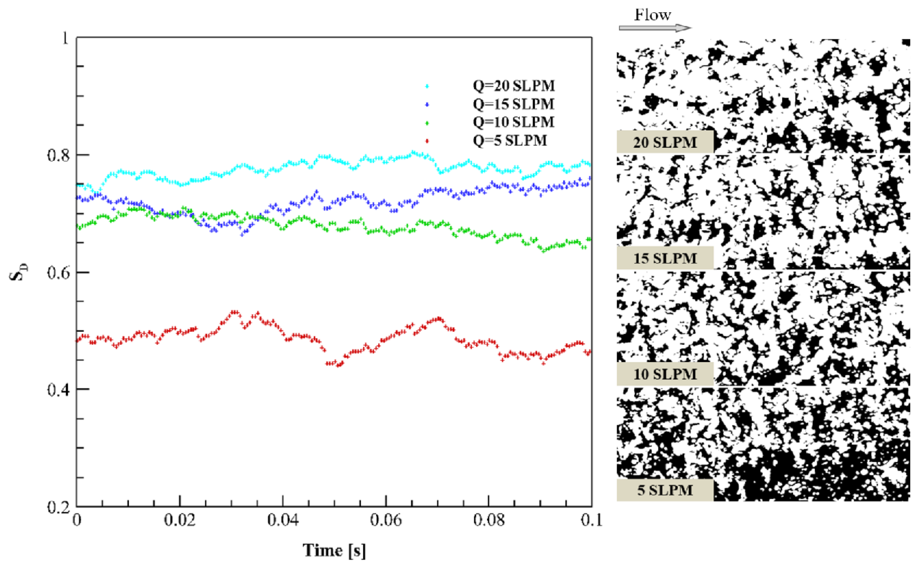
3.1. Single-Bubble Tracking and Spatial Density

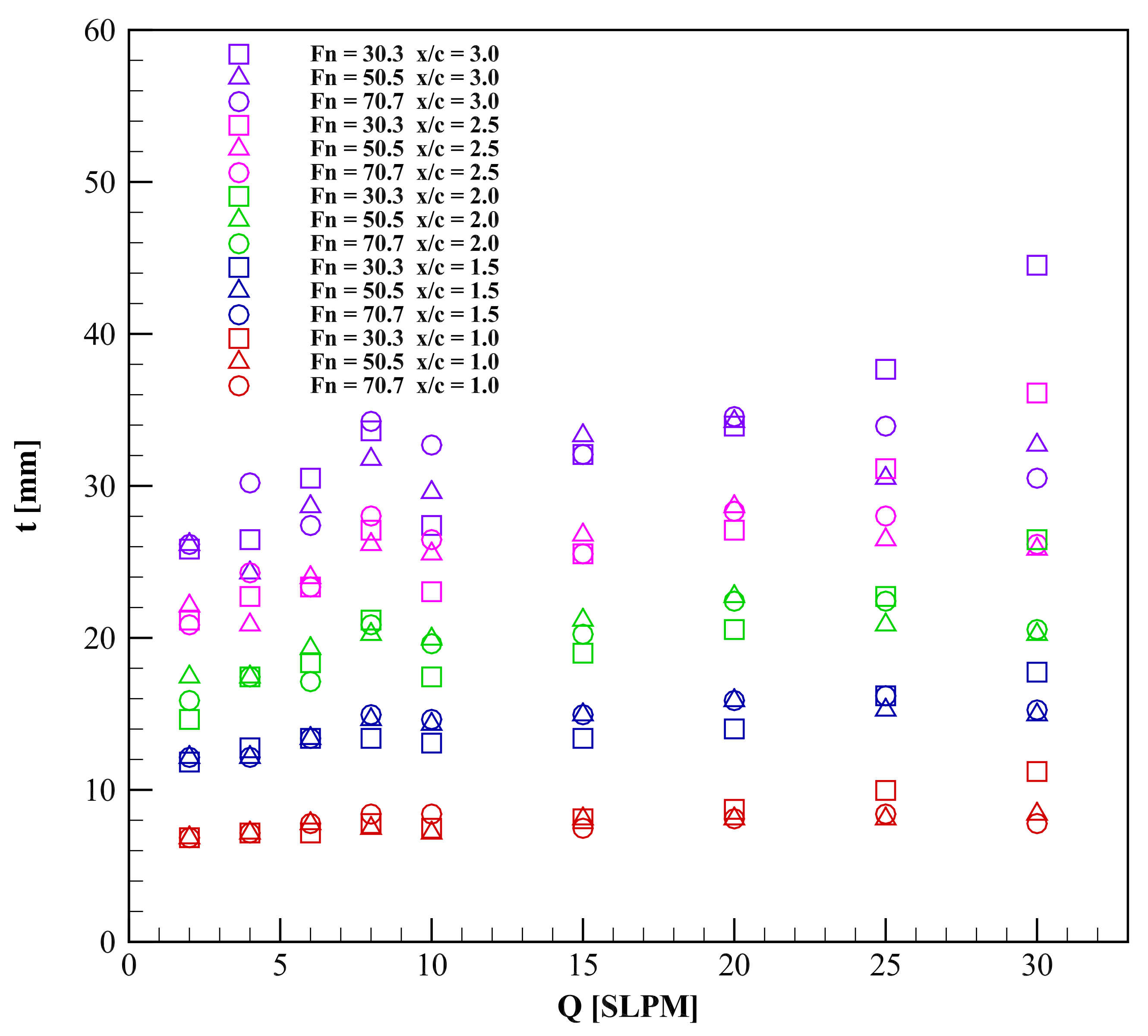
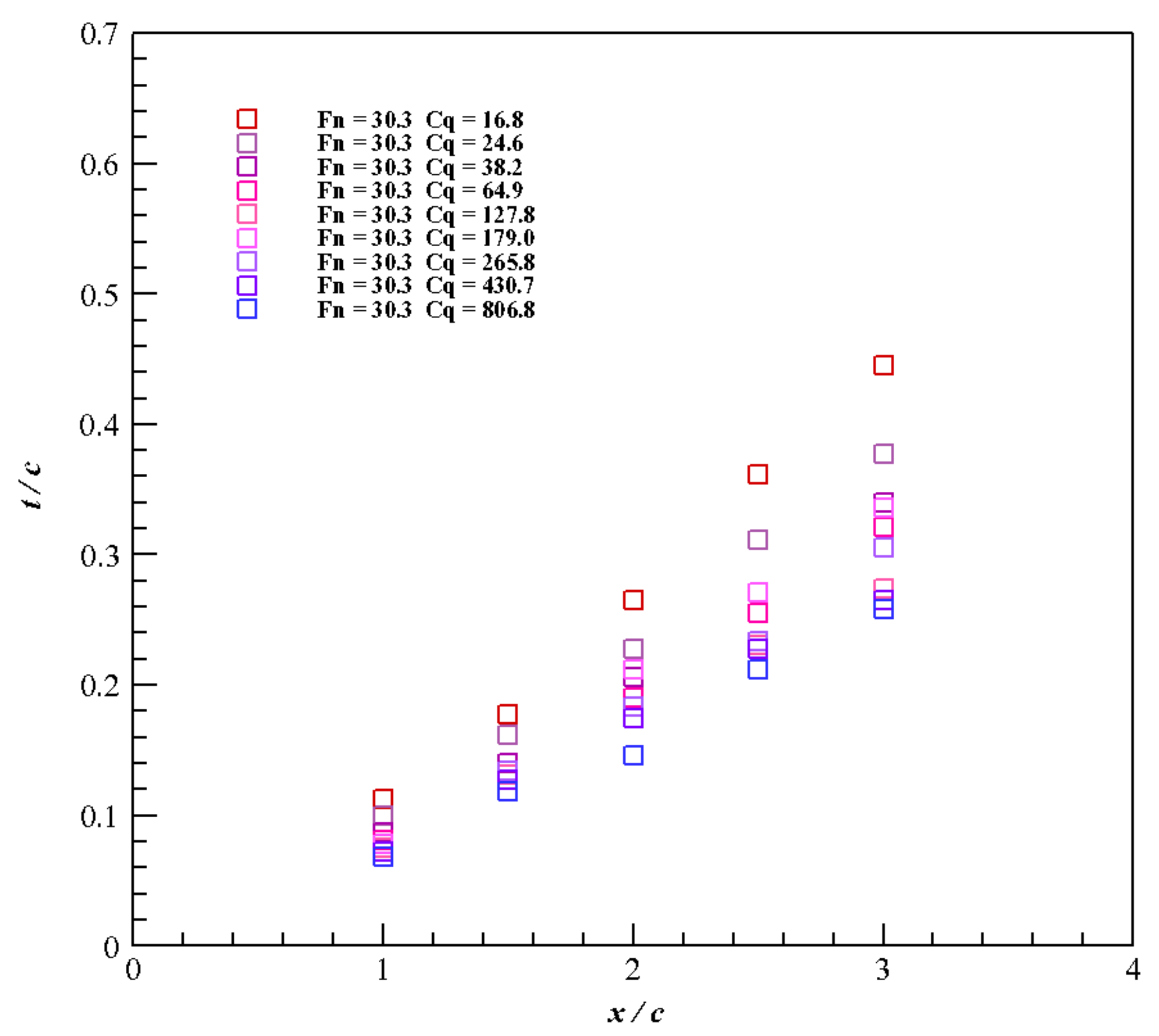
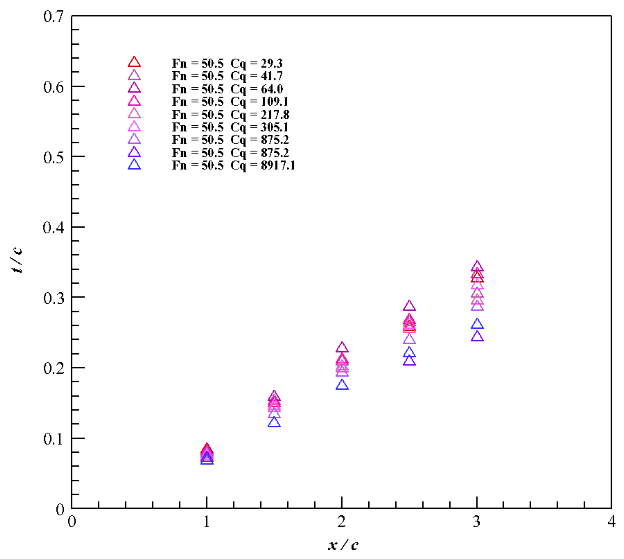
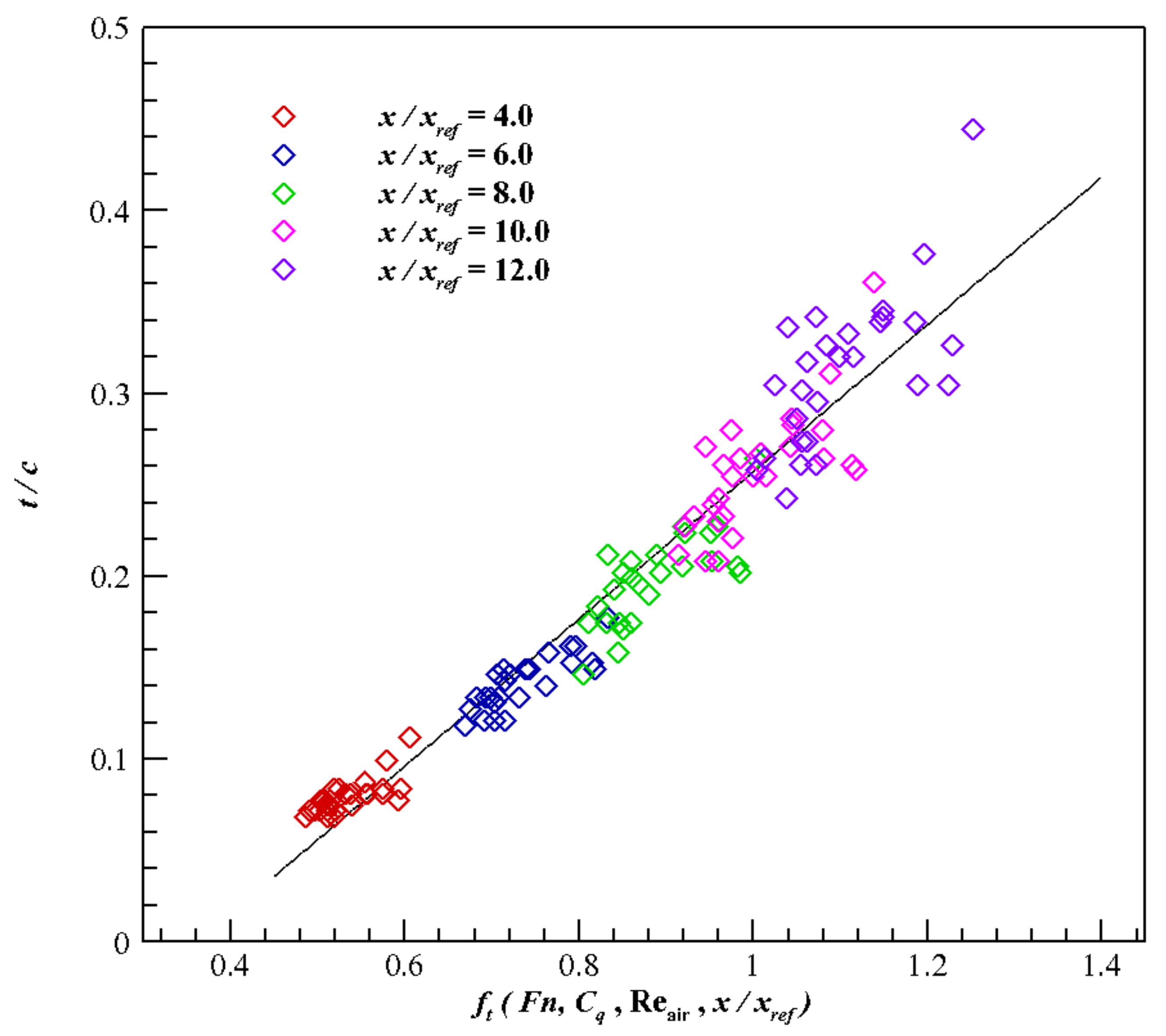
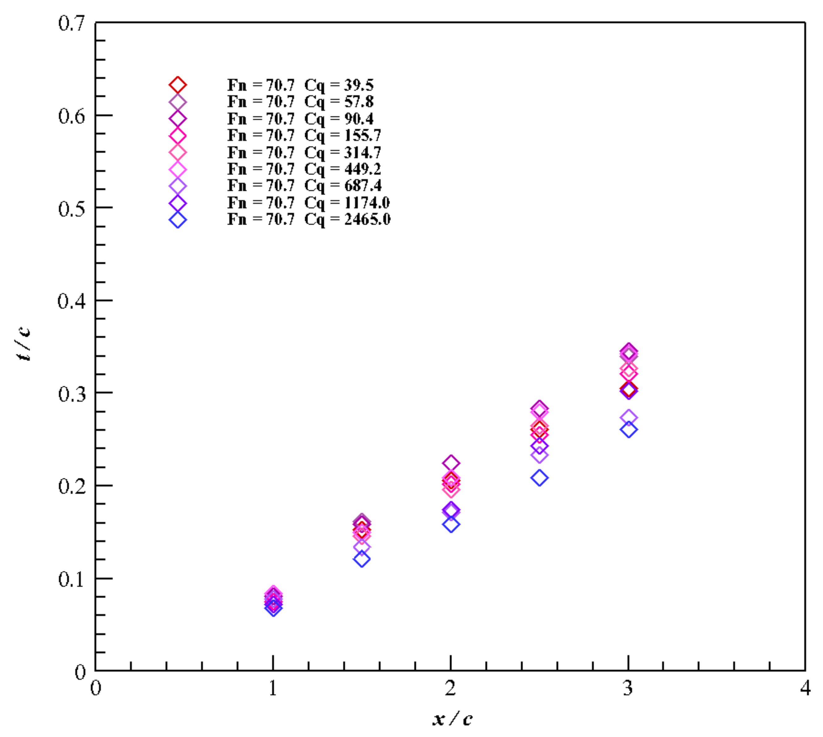
Individual bubbles emanating through air injection vents on the hydrofoil were tracked using a 2D image processing algorithm called the Channel and Spatial Reliability Tracking (CSRT) algorithm in OPENCV-Python, whose flowchart is shown in Figure 5. The algorithm for single-bubble tracking was designed such that a tracker was initiated in the CSRT algorithm upon designating the Region of Interest (ROI) as shown in Figure 5 and the tracker and ROI initialized successively for each frames in the high-speed video; thus, keeping track of an individual bubble as it was advected over time in the observation window. The algorithm for finding the spatial density, $S_D$, in the observation window is shown in Figure 6, where the high-speed images were extracted from the high-speed video and a threshold was set in order to generate binary images from RGB images. The individual frames from the original high-speed video were extracted and the Red–Green–Blue (RGB) frames were transformed into grayscale frames by a difference image technique, where the RGB frame was subtracted from a background frame. The grayscale frames were binarized and a bubble segmentation was performed to find the contours in the binary frames. The high-speed video was input into the CSRT algorithm tracker and the region of interest was designated. Then, the region of interest and the trackers were initialized, and the tracker was updated for every frame. The algorithm also enhanced the resolution at the edges, resulting due to background noise and a non-uniform brightness from illumination. Thus, a single air bubble was tracked over time and its dimension in terms of the number of pixels it occupied on a given frame was determined over time. The algorithm was validated by creating artificial frames containing circles of a known radius and moving at a known translation rate and deformation rate across the frames, and it was found that the errors involved in the calculation of the bubble size and spatial density, $S_D$, were minimum.

The bubble size of one of the air bubbles in the pixels is shown to vary over time in Figure 7 (multimedia view). Even as the bubble was advected along the flow, it rolled about in space and a variation in the bubble size was observed over time. The drop in the bubble size towards the end of the time series was because the bubble reached the end of the observation area. Based on the measured bubble size, the deformation rate of the individual bubbles was defined as in Equation (1), where $P_t$ was the pixels covered by an air bubble at a given instant of time, and $P_i$ was the pixels covered by an air bubble at an initial time. The measured bubble size in the pixels was standardized as in Equation (2), where $P_t$ was the bubble size at an instant in time, $<P>$ was the time-averaged bubble size at a given instant of time, and $\sigma (P)$ was the standard deviation of the bubble size. The plot of the measured deformation rate, $ϵ$, and standardization, ${ϵ}_s$, over time for several bubbles is shown varying over time in Figure 8 and Figure 9. A variation of $ϵ$ and ${ϵ}_s$ with time was detected, even as they advected along with the free-stream.

$$ϵ=\frac{P_t-P_i}{P_i}$$

(1)

$${ϵ}_S=\frac{P_t-<P>}{\sigma (P)}$$

(2)

A quantity called spatial density was defined in order to quantify the area occupied by the bubbles per unit area of view. It was the ratio of the number of pixels with a value of unity in a binary image, $\Sigma (P_1)$, to the total number of pixels in the image, where $P_1$ is the pixels with the value unity, as given in Equation (3). The images obtained in each step of binarization are shown in Figure 10. The spatial density of the bubbles was computed at various air injection rate and free-stream velocity combinations. For all the experimental runs, the spatial density was observed to vary with time even as bubbles of various size were advected along with the free-stream flow in the observation window. At a low free-stream velocity of 3 m/s, the spatial density was low at $Q=5SLPM$; upon a further increase in the air injection rate, at $Q=10,15,20SLPM$, the spatial density of the bubbles nearly remained constant as shown in Figure 11. The explanation for $S_D$ remaining nearly constant with time for different Q at $V_{\infty }=3$ m/s may be attributed to considerable buoyancy effects at a low free-stream velocity. The binary frames corresponding to various air injection rates at the Froude number of 30.3 are shown in Figure 11. A variation of spatial density with time for the Froude numbers 50.5 and 70.7 is shown in Figure 12 and Figure 13. It was observed that, at a given free-stream velocity, $V_{\infty }=5$ m/s, 7 m/s, there was an increase in the spatial density with an increase in Q for larger free-stream velocities as shown in Figure 12 and Figure 13.

Taking a time average of the spatial density, we observed the time-averaged spatial density, $<S_D>$, varying in a linear manner with the logarithm of the air injection rate, $ln(Q)$, at various free-stream velocities as shown in Figure 14. The linear fit between the time-averaged spatial density, $<S_D>$, and the logarithm of the air injection coefficient had a coefficient of determination, $R^2$, values equal to 0.4, 0.92 and 0.92, respectively, for $Fn=30.3,50.5$ and 70.7, respectively, indicated by red, green and blue lines in Figure 14. The regression analysis of the time-averaged spatial density, $<S_D>$, was performed with a view to find its dependence on the non-dimensional governing parameters, Froude number, $Fn$, air injection coefficient, $C_q$, and Reynolds number, ${Re}_{air}$. A power–law relation was found for the time-averaged spatial density, $<s_D>$, as given in Equation (4) with a linear fit between the model computed values and the experimental observations, as shown in Figure 15 with $R^2=0.93$. The increase in the time-averaged spatial density with the increase in velocity at a given air injection coefficient and the increase in the time-averaged spatial density with the increase in the air injection coefficient at a given free-stream velocity as observed in Figure 14 were both evident from the exponents of the non-dimensional independent variables in Equation (4).

$$S_D=\frac{\Sigma (P_1)}{Totalpixels}$$

(3)

$$f_{SD}={Fn}^{1.76}{C}_q^{-0.68}{Re}_{air}^{-0.49}$$

(4)

3.2. Jet Thickness

The time-averaged thickness of the jet was observed from the top-view images at the angles of inclination, $\alpha$ = 3.5°, at various air injection rates, Q, and free-stream velocities, $V_{\infty }$. The plot of the time-averaged jet thickness, t, at various combinations of Q and $V_{\infty }$ values, at the angle of inclination of $\alpha$ = 3.5° is shown in Figure 16. The jet thickness increased with the increase in the downstream distance from the trailing edge of the hydrofoil at all free-stream velocities and the air injection coefficient values. It was observed that there was an increase in the jet thickness with the increase in the air injection coefficient at all free-stream velocities and at all non-dimensional streamwise distances from the trailing edge of the hydrofoil ($x/c=0$) in Figure 16. Figure 17 shows the variation of the non-dimensional jet thickness, $t/c$, along the non-dimensional streamwise distance, $x/c$, for various non-dimensional air injection rates, $C_q$, at the Reynolds number, ${Re}_{air}=30.3$. In general, at a given non-dimensional streamwise distance, $x/c$, it was observed that the non-dimensional jet thickness, $t/c$, increased with the decrease in the non-dimensional air injection rate, $C_q$, at ${Re}_{air}=30.3$. It is to be noted that $C_q$ was inversely proportional to Q, based on our definition in Section 2. Further, at ${Re}_{air}=30.3$, the non-dimensional jet thickness, $t/c$, was observed to increase along the non-dimensional streamwise distance, $x/c$, at a given non-dimensional air injection rate, $C_q$. Similarly, Figure 18 and Figure 19 show the variation of the non-dimensional jet thickness, $t/c$, along the non-dimensional streamwise distance, $x/c$, for various non-dimensional air injection rates, $C_q$, at the Reynolds number, ${Re}_{air}=50.5,70.7$, respectively. The characteristic of the jet, namely, the increase in the non-dimensional jet thickness along the streamwise direction with the decrease in the non-dimensional air injection rate, $C_q$, at a fixed non-dimensional distance from the trailing edge, was observed for $Re=50.5,70.7$ as well in Figure 18 and Figure 19. Similarly, there was an increase in the non-dimensional jet thickness, $t/c$, along the non-dimensional streamwise distance, $x/c$, at a given non-dimensional air injection rate, $C_q$, for $Re=50.5,70.7$ as well in Figure 18 and Figure 19.

A regression analysis was performed on the non-dimensional jet thickness, $t/c$, based on the non-dimensional parameters, Froude number, $Fn$, and air injection coefficient, $C_q$, Reynolds number, ${Re}_{air}$, and non-dimensional streamwise distance, $x/x_{ref}$. $x_{ref}$ was taken as the horizontal distance from the leading edge to the position of the maximum thickness on the hydrofoil in order to be conducive for the regression analysis; $x_{ref}=25$ mm for NACA 0010 hydrofoil having a chord length of 100 mm. The equation for the non-dimensional jet thickness was given by (5) in terms of the non-dimensional parameters $Fn,C_q{Re}_{air}$ and $x/x_{ref}$. The straight line in Figure 20 shows a linear fit between the power–law model and experimental observations, with a coefficient of determination, $R^2=0.9$. The observed behavior of the non-dimensional time-averaged jet width, which was an increase with the increase in the air injection rate, Q, at a constant free-stream velocity, $V_{\infty }$, and a decrease with the increase in the free-stream velocity, $V_{\infty }$, at a constant air injection rate, Q, as observed in general through Figure 16, Figure 17, Figure 18 and Figure 19, was evident from the exponents of the non-dimensional independent variables in Equation (5).

$$f_t=F{n}^{0.48}{C}_q^{-0.49}R{e}_{air}^{-0.42}{(x/x_{ref})}^{1.24}$$

(5)

4. Conclusions

In this work, we characterized bubbles flowing through multiple vents on the surface of an inclined hydrofoil in a free-stream. The effect of buoyancy was evident at low non-dimensional air injection rates, $C_q$, and low Froude numbers, $Fn$. The variation of the bubble size in pixels was obtained with time by image processing. Based on the bubble size, the deformation rate, $ϵ$, and standardization, ${ϵ}_s$ was observed to change with time, even as the bubble was advected by the free-stream. By image processing, the packing of the bubbles in a unit area was quantified in terms of spatial density, $S_D$. The spatial density was observed to vary with time at several combinations of the Froude number, $Fn$, and non-dimensional air injection coefficients, $C_q$. The time-averaged spatial density was observed to increase in general with the increase in the air injection rate at all Froude numbers in a logarithmic manner. We obtained a power–law relation for the time-averaged spatial density with the non-dimensional parameters such as, $Fn,C_q$ and $R{e}_{air}$. The thickness, t, of the jet was observed based on the top view images. The thickness of the jet was observed to increase monotonically with the increase in the air injection rates in general, at all free-stream velocities, at all distances downstream of the hydrofoil. A power–law relation was obtained based on the regression analysis for the non-dimensional jet thickness in terms of $Fn,C_q,R{e}_{air}$ and $x/x_{ref}$. Such a study on bubble dynamics, due to multi-vent injection, is necessary for engineering applications that involve air injection in water.

References

1. Elbing, B.R.; Winkel, E.S.; Lay, K.A.; Ceccio, S.L.; Dowling, D.R.; Perlin, M. Bubble-induced skin-friction drag reduction and the abrupt transition to air-layer drag reduction. J. Fluid Mech. 2008, 612, 201. [Google Scholar] [CrossRef]
2. Yanuar, Y.; Waskito, K.T.; Gunawan, G.; Candra, B.D.; Perdana, A.Y. Micro-bubble Drag Reduction by Multi Discrete Hole Plate on Self Propelled Barge Ship Model. J. Adv. Res. Fluid Mech. Therm. Sci. 2019, 53, 111–121. [Google Scholar]
3. Ohashi, H.; Matsumoto, Y.; Ichikawa, Y.; Tsukiyama, T. Air/water two-phase flow test tunnel for airfoil studies. Exp. Fluids 1990, 8, 249–256. [Google Scholar] [CrossRef]
4. Ayers, R.R.; Jones, W.T.; Hannay, D. Methods to Reduce Lateral Noise Propagation from Seismic Exploration Vessels. Int. Conf. Offshore Mech. Arct. Eng. 2009, 43451, 111–122. [Google Scholar]
5. Kumagai, I.; Nakamura, N.; Murai, Y.; Tasaka, Y.; Takeda, Y.; Takahashi, Y. Numerical investigation on theA new power-saving device for air bubble generation: Hydrofoil air pump for ship drag reduction. In Proceedings of the International Conference on Ship Drag Reduction SMOOTH-SHIPS, Istanbul, Turkey, 20–21 May 2010. [Google Scholar]
6. Kumagai, I.; Takahashi, Y.; Murai, Y. Power-saving device for air bubble generation using a hydrofoil to reduce ship drag: Theory, experiments, and application to ships. Ocean Eng. 2015, 95, 183–194. [Google Scholar] [CrossRef] [Green Version]
7. Amromin, E.; Karafiath, G.; Metcalf, B. Ship drag reduction by air bottom ventilated cavitation in calm water and in waves. J. Ship Res. 2011, 55, 186–193. [Google Scholar] [CrossRef]
8. Wu, H.; Ou, Y.-P. Experimental Study of Air Layer Drag Reduction with Bottom Cavity for A Bulk Carrier Ship Model. China Ocean Eng. 2019, 33, 54–562. [Google Scholar]
9. Jang, J.; Choi, S.H.; Ahn, S.-M.; Kim, B.; Seo, J.S. Experimental investigation of frictional resistance reduction with air layer on the hull bottom of a ship. Int. J. Nav. Archit. Ocean. Eng. 2014, 6, 363–379. [Google Scholar] [CrossRef] [Green Version]
10. Mohanarangam, K.; Cheung, S.C.P.; Tu, J.Y.; Chen, L. Numerical simulation of micro-bubble drag reduction using population balance model. Ocean Eng. 2009, 36, 863–872. [Google Scholar] [CrossRef]
11. Mizokami, S.; Kawakita, C.; Kodan, Y.; Takano, S.; Higasa, S.; Shigenaga, R. Experimental study of air lubrication method and verification of effects on actual hull by means of sea trial. Mitsubishi Heavy Ind. Tech. Rev. 2010, 47, 41–47. [Google Scholar]
12. Murai, Y.; Sakamaki, H.; Kumagai, I.; Park, H.J.; Tasaka, Y. Mechanism and performance of a hydrofoil bubble generator utilized for bubbly drag reduction ships. Ocean Eng. 2020, 216, 108085. [Google Scholar] [CrossRef]
13. Mäkiharju, S.A.; Perlin, M.; Ceccio, S.L. On the energy economics of air lubrication drag reduction. Int. J. Nav. Archit. Ocean. Eng. 2012, 4, 412–422. [Google Scholar] [CrossRef] [Green Version]
14. Karn, A.; Ellis, C.R.; Milliren, C.; Hong, J.; Scott, D.; Arndt, R.E.; Gulliver, J.S. Bubble size characteristics in the wake of ventilated hydrofoils with two aeration configurations. Int. J. Fluid Mach. Syst. 2015, 8, 73–83. [Google Scholar] [CrossRef]
15. Han, J.; Vahaji, S.; Cheung, S.C. Numerical investigation on the influencing interphase forces on bubble size distribution around NACA0015 hydrofoil. Exp. Comput. Multiph. Flow 2019, 1, 145–157. [Google Scholar] [CrossRef] [Green Version]
16. Murai, Y. Frictional drag reduction by bubble injection. Exp. Fluids 2014, 55, 1–28. [Google Scholar] [CrossRef]
17. Yu, A.; Qian, Z.; Wang, X.; Tang, Q.; Zhou, D. Large Eddy simulation of ventilated cavitation with an insight on the correlation mechanism between ventilation and vortex evolutions. Appl. Math. Model. 2021, 89, 1055–1073. [Google Scholar] [CrossRef]
18. Wang, H.; Dong, F. Track of rising bubble in bubbling tower based on image processing of high-speed video. In Proceedings of the International Society for Optical Engineering, Beijing, China, 10–13 October 2008. [Google Scholar] [CrossRef]
19. Ying, H.; Puzhen, G.; Chaoqun, W. Experimental and numerical investigation of bubble-bubble interactions during the process of free ascension. Energies 2019, 12, 1977. [Google Scholar] [CrossRef] [Green Version]
20. Cheng, D.-C.; Burkhardt, H. Bubble tracking in image sequences. Int. J. Therm. Sci. 2003, 42, 647–655. [Google Scholar] [CrossRef]
21. Acuna, C.A.; Finch, J.A. Tracking velocity of multiple bubbles in a swarm. Int. J. Miner. Process. 2010, 94, 147–158. [Google Scholar] [CrossRef]
22. Oishi, Y.; Murai, Y.; Tasaka, Y.; Yasushi, T. Frictional drag reduction by wavy advection of deformable bubbles. J. Phys. Conf. Ser. 2009, 147, 012020. [Google Scholar] [CrossRef]
23. Nagarathinam, D.; Kim, K.; Ahn, B.-K.; Park, C.; Kim, G.-D.; Yim, G.-T. Experimental investigation of bubbly flow by air injection on an inclined hydrofoil. Phys. Fluids 2021, 33, 043309. [Google Scholar] [CrossRef]
24. Walton, D.; Spence, M.K.; Reynolds, B.T. The effects of free stream air velocity on water droplet size and distribution for an impaction spray nozzle. J. Power Energy 2000, 214, 531–537. [Google Scholar] [CrossRef]
Figure 1. Schematic of the current experimental setup. Detail of the air injection vents is shown in the inset.
Applsci 11 09890 g001
Figure 2. The instantaneous images showing the bubbles at F n = 30.3 for Q = 6 to 20 S L P M . (a) Side view at Q = 10 S L P M . (b) Top view at Q = 10 S L P M . (Multimedia view).
Applsci 11 09890 g002
Figure 3. The instantaneous images showing the bubbles at F n = 50.5 at Q = 6 to 20 S L P M . (a) Side view at Q = 10 S L P M . (b) Top view at Q = 10 S L P M . (Multimedia view).
Applsci 11 09890 g003
Figure 4. The instantaneous images showing the bubbles at F n = 70.7 at Q = 6 to 20 S L P M . (a) Side view at Q = 10 S L P M . (b) Top view at Q = 10 S L P M . (Multimedia view).
Applsci 11 09890 g004
Figure 5. The schematic of the algorithm for tracking an individual bubble over time.
Applsci 11 09890 g005
Figure 6. The algorithm utilized for evaluating spatial density, S D , in the observation window for any generic case.
Applsci 11 09890 g006
Figure 7. Bubble size in pixel over time, as it is advected with the free-stream (multimedia view).
Applsci 11 09890 g007
Figure 8. Deformation rate, ϵ , is shown over time for several marked bubbles at V = 3 m/s, Q = 5 S L P M .
Applsci 11 09890 g008
Figure 9. Standardization, ϵ S , is shown over time for several marked bubbles at V = 3 m/s, Q = 5 S L P M .
Applsci 11 09890 g009
Figure 10. Binarization process of the RGB image into a binary image. The arrow indicates the direction of the free-stream velocity vector.
Applsci 11 09890 g010
Figure 11. Change of spatial density with time at the free-stream velocity of 3 m/s for various air injection rates. The arrow indicates the direction of the free-stream velocity vector.
Applsci 11 09890 g011
Figure 12. Change of spatial density with time at the free-stream velocity of 5 m/s for various air injection rates. The arrow indicates the direction of the free-stream velocity vector.
Applsci 11 09890 g012
Figure 13. Change of spatial density with time at the free-stream velocity of 7 m/s for various air injection rates. The arrow indicates the direction of the free-stream velocity vector.
Applsci 11 09890 g013
Figure 14. The linear variation of the time-averaged spatial density, < S D > , with the logarithm of the air injection rate, l n ( Q ) , at different Froude numbers, F n . R 2 values for F n equal to 70.7, 50.5 and 30.3 were equal to 0.92, 0.92 and 0.4, respectively.
Applsci 11 09890 g014
Figure 15. The time-averaged spatial density, < S D > is shown against f S D , which is a function of Froude number, F n , air injection coefficient, C q , and Reynolds number, R e a i r . The linear fit between the experimental measurements and the power–law model is indicated by a straight line having R 2 = 0.93 .
Applsci 11 09890 g015
Figure 16. The jet thickness at various air injection rates, Q, and free-stream velocity, V .
Applsci 11 09890 g016
Figure 17. The non-dimensional jet thickness, t / c , variation along the non-dimensional stream-wise distance, x / c , for various non-dimensional air injection rates, C q , at Reynolds number, R e a i r = 30.3 .
Applsci 11 09890 g017
Figure 18. The non-dimensional jet thickness, t / c , variation along the non-dimensional stream-wise distance, x / c , for various non-dimensional air injection rates, C q , at Reynolds number, R e a i r = 50.5 .
Applsci 11 09890 g018
Figure 19. The non-dimensional jet thickness, t / c , variation along the non-dimensional stream-wise distance, x / c , for various non-dimensional air injection rates, C q , at Reynolds number, R e a i r = 70.7 .
Applsci 11 09890 g019
Figure 20. The non-dimensional jet thickness, t / c , was plotted against f t , which was a function of Froude number, F n , and air injection coefficient, C q , Reynolds number, R e a i r , and non-dimensional streamwise distance, x / x r e f , with the colors in red, blue, green, magenta and violet representing x / x r e f = 4 , 6 , 8 , 10 and 12, respectively. The R 2 value for the linear curve fit was 0.94.
Applsci 11 09890 g020
Publisher’s Note: MDPI stays neutral with regard to jurisdictional claims in published maps and institutional affiliations.