Anomaly Detection in Automotive Industry Using Clustering Methods—A Case Study

Featured Application

Parts grouping “Clustering” by master data similarity on automotive industry. Anomaly detection on material classification. Machine learning clustering algorithms comparison—Study Case. Clustering quality index techniques comparison.

Abstract

In automotive industries, pricing anomalies may occur for components of different products, despite their similar physical characteristics, which raises the total production cost of the company. However, detecting such discrepancies is often neglected since it is necessary to find the problems considering the observation of thousands of pieces, which often present inconsistencies when specified by the product engineering team. In this investigation, we propose a solution for a real case study. We use as strategy a set of clustering algorithms to group components by similarity: K-Means, K-Medoids, Fuzzy C-Means (FCM), Hierarchical, Density-Based Spatial Clustering of Applications with Noise (DBSCAN), Self-Organizing Maps (SOM), Particle Swarm Optimization (PSO), Genetic Algorithm (GA) and Differential Evolution (DE). We observed that the methods could automatically perform the grouping of parts considering physical characteristics present in the material master data, allowing anomaly detection and identification, which can consequently lead to cost reduction. The computational results indicate that the Hierarchical approach presented the best performance on 1 of 6 evaluation metrics and was the second place on four others indexes, considering the Borda count method. The K-Medoids win for most metrics, but it was the second best positioned due to its bad performance regarding SI-index. By the end, this proposal allowed identify mistakes in the specification and pricing of some items in the company.

1. Introduction

Efficiency in the cost management at the automotive companies is extremely important to generate competitive products in a global open market. Financial and managerial successes are linked to a fast adaption to current daily challenges, with free competition. Innovative products with reduced launch times are frequently requested, and customers perceive a high quality. Moreover, flexibility and competitive prices are prerequisites to survive in the automotive business. These challenges are increasingly present in the industry and mainly influence a company’s responsiveness, versatility, speed and adaptability to changes. Simultaneously, the industry is always looking for cost reduction [1,2,3].

This scenario leads to constant launches of new vehicles with new configurations and options. However, low production volumes in specific configurations increase the costs due to manufacturing complexity. This often leads to decentralization in the engineering sector by a product family, which leads to the development of components with minor design changes and possibly triggering a significant increase in manufacturing cost [4,5,6,7].

Many variables in the manufacturing processes and the composition of products in the automotive industry generate several combinations and configurations daily, making it impossible to process them manually. As a large volumes of data are generated, much of the potential knowledge achieved is not directly applied to similar items [3,8].

Due to the advancement of information and management systems technology in the production chain, there is a significant increase in the amount of data generated, collected, and stored in various applications [9,10,11]. Therefore, efficient tools that automatically execute knowledge discoveries are useful in large data sets, especially those with complexity and heterogeneity [12,13,14].

However, there is a lack of methodologies that recognize similarities among the many items in the automotive industry and group it adequately to identify pricing and classification anomalies.

The work developed by Pan and Lu [15] proposed constructing a model for grouping parts to replace the conventional manufacturing process by additive manufacturing (AM). The current evaluations of (AM) are manually done, which reduces the scope of the application. In this model, the grouping of components is done automatically by clustering algorithms for other manufacturing processes by additive manufacturing (AM).

On Zhong, Xu and Pan [16] developed a non-threshold consensus model that combines the minimum cost and maximum consensus-increasing for multi-attribute large-group decision-making (MALGDM). The main differences between traditional clustering techniques is that instead of using a predefined threshold and a maximum number of iterations, a termination index is developed to terminate the consensus reaching process (CRP), considering different consensus metrics.

In addition, Kong et al. [17] introduced a two-mode modularity clustering method with new similarity measures for parts and machines using an ordinal part-machine matrix. The proposed method considers both incidences, transition between parts and machines and find optimal clusters. The method produces reasonable cell formation solutions in terms of several performance measures.

Bodendorf, Merkl and Franke [18] make a literature review on intelligent cost estimation methods for parts to be procured in the manufacturing industry is carried out by text mining. Consequently, in this paper, approaches derived from Multitask Learning and Explainable Machine Learning can be found. A combination of methods considered most suitable for predictive analytics to estimate procurement costs is presented.

Finally, Chan, Lu and Wangon [19] developed a new cost estimation framework based on big data analytics tools. The manufacturing cost associated with a new job can be estimated based on similar ones in the past. The new framework is implemented and demonstrated for additive manufacturing, where the similarities of the 3D geometry of parts and printing processes are established by identifying relevant features.

In this sense, a challenge for identifying pricing anomalies is to monitor whether the classifications (labels) available in the registration data are adequate for the correct grouping of parts, which should have similar manufacturing costs. In the case study addressed here, two classifications previously existing in the database were evaluated, the NCM and the class number. The NCM, which is an acronym for Mercosur Common Nomenclature, is a hierarchical code of categories. Brazilian taxes, descriptions, and rates are attached to each NCM code [20,21,22]. The class number is data created by product engineering when creating new parts. The product engineers freely choose the definition of this number. Consequently, it presents a subjective character, being susceptible to different interpretations. Both labels may show inconsistencies during the sample analysis.

In this investigation, we address an actual case study from an automaker. Nowadays, there is an immediate need to expand the company’s focus to include analyzing large sample sets, which can be multidimensional and complex for manual analysis.

This way, clustering techniques are used to identify pricing anomalies in similar parts, using their specifications as a basis. Clustering methods are tools used on many research fronts, including data mining so that significant knowledge is extracted from apparently unstructured samples [23,24,25,26]. In addition, clustering is a way to group data and identify patterns coherently and unsupervised [27,28]. Among the different techniques, the literature points out those computational intelligence techniques are an alternative to traditional methods such as K-Means in real problems. However, the current knowledge about this task is not enough to define the best algorithm for all cases [10,23,29].

Based on these premises, several clustering approaches are addressed, namely: K-means, K-Medoids, Fuzzy C-means (FCM), Hierarchical, Density-Based Spatial Clustering of Applications with Noise (DBSCAN), Self-Organizing Maps (SOM), Particle Swarm Optimization (PSO), Genetic Algorithm (GA) and Differential Evolution (DE). As evaluation and comparison metrics, the following indices are used: Sum of Squared Errors (SSE), Sum of Squares Within Clusters (SSW), Sum of Squares Between Clusters (SSB), Calinski-Harabasz (CH), WB, and Silhouette index.

To the best of our knowledge, the use of clustering methods for anomaly detection considering components of an automaker is an unprecedented proposal as a case study. Therefore, this study contributes to an understanding of complex data related to group parts without knowing the classification in advance. It also extends the experience to the existing knowledge through previous research.

This paper was organized as follows. Section 2 presents a description of each technique used; Section 3 shows the metrics used for cluster quality evaluation, while Section 4 presents the database, results, and critical analysis. The conclusions are in Section 5.

2. Clustering Algorithms

2.1. K-Means

The K-Means is a well-known clustering algorithm because it is easy to implement and understand, requests low computational effort, and presents fast convergence [10,30]. It has been adapted to many challenging problems in distinct domains [31,32].

The K-Means initialization starts with the random generation of the centroids’ position. The data are allocated to each group, and then a given sample will belong to the cluster with the shortest distance to the respective centroid. After this phase, the new positions of the centroids are recalculated, and they move to the geometric center of the cluster formed in the current iteration [9].

The algorithm runs to minimize the sum of the internal distance (Sum of Squares Within Clusters—SSE) between the data and the centroids by Equation (1). In this equation, the measure dist is the Euclidean distance given by Equation (2):

$$SSE={\displaystyle \sum }_{k=1}^K{\displaystyle \sum }_{i=1}^{n_q}dist{\left(x_i-c_k\right)}^2$$

(1)

where c_k is the centroid of cluster k, x_i is the i-th object of the k-th cluster, K is the number of clusters, and n_q is the number of elements on each cluster and

$$dist\left(x_i, c_k\right)=\sqrt{{\displaystyle \sum }_{d=1}^D{\left(x_{i,d}-c_{k,d}\right)}^2}$$

(2)

where d is each number of dimensions of each object on the data set, and D represents the last dimension of each object [10].

$$c_k=\frac{1}{n_k}{\displaystyle \sum }_{i=1}^{n_k}{x}_i^k$$

(3)

where n_k is the number of objects in the respective cluster.

This process is repeated until a stop criterion is reached. The most used are the number of iterations or a predefined limit of a similarity measure.

We highlight that the strong dependence on the initialization is widely known. In addition, the user must specify the number of clusters a priori [25,33].

2.2. K-Medoids

Another method of partial grouping is K-Medoids [34], in which a data set X is stored in K clusters. This algorithm minimizes the differences between each object in a cluster and its representative object (centroid), similar to the K-Means.

Initially, centroids need to be defined, in this case, known as Medoids. The most common way to proceed with this step is to determine as centroids n_k samples from the data group, drawn randomly. This is done to minimize the effects of K-Means random initialization [35].

Thus, it is expected to find a single partition of the data in the K clusters. Each one has a more representative point: the most centrally located concerning some measure, for example, Euclidean distance [36]. Such an idea reduces noise and discrepancies, making the method more robust than K-Means [35]. The execution steps are like the K-Means case.

2.3. Fuzzy C-Means (FCM)

Fuzzy C-Means (FCM) has become an essential method with many grouping-clustering applications for real-world problems [37]. Among the diffuse clustering methods, FCM is one of the best known for its simplicity and efficiency. However, it shows some weaknesses, particularly its tendency to fall to local lows at minimum local points.

This algorithm treats clusters as flexible groups in which each data object has presented a degree of association. These degrees are evaluated between 0 and 1, with a high value representing a high degree of similarity between the current object under study and the group [38].

According to [39], FCM has shown important characteristics: the number of groups can be defined automatically; it works well with overlapping data and is robust for initialization, noise, and outliers.

The FCM defines an association matrix $U={\left\{u_{ij}\right\}}_{i,j}^{N, n_k}$, where u_ij ∈ [0, 1] is the degree of membership, ${{\displaystyle \sum }}_{j=1}^{n_k}{u}_{ij}$, ∀i, and $0<{{\displaystyle \sum }}_{i=1}^N{u}_{ij}<N$, being N the number of objects. Note that each pattern is named i for each cluster j and n_k is the number of objects in the respective cluster.

The objective of the method is to minimize the cost function J_m described in Equation (4):

$${\mathit{J}}_m={\displaystyle \sum }_{i=1}^N{\displaystyle \sum }_{j=1}^{n_k}{u}_{ij}^m\Vert x_i-c_j{\Vert }^2$$

(4)

in which ‖.‖ it is usually the Euclidean norm, and m is the inaccuracy coefficient provided by the user.

After that, the degree of relevance and the central positions are calculated by Equations (5) and (6):

$$u_{ij}^m=\frac{1}{{{\displaystyle \sum }}_{k=1}^C{\frac{\Vert x_i-c_j\Vert }{\Vert x_i-c_k\Vert }}^{\frac{2}{m-1}}}$$

(5)

$$c_j=\frac{{{\displaystyle \sum }}_{i=1}^N{u}_{ij}^m.x_i}{{{\displaystyle \sum }}_{i=1}^N{u}_{ij}^m}$$

(6)

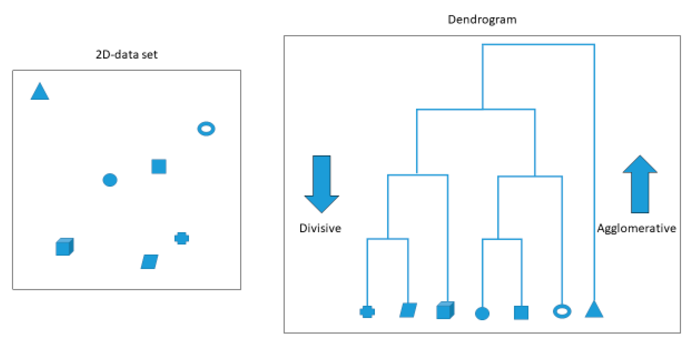
2.4. Hierarchical Clustering

Hierarchical clustering algorithms generate groups at successive levels, in which the current grouping process is created based on the previous hierarchical level. Unlike the partial approach, hierarchical clustering does not need to specify the number of clusters in advance [13].

However, the computational cost required to perform these methods is high, which is unfeasible for a large data set. Hierarchical approaches create a dendrogram structure, consisting of a tree structure representing the hierarchical sequence of nested partitions of the data set [14]. The procedure creates successive cluster levels, in which the current group is based on the solution obtained in the previous level [40].

There are two types of hierarchical algorithms: divisive and agglomerative [41,42]. In the divisive case, the process begins with all data elements in a single cluster divided into smaller clusters based on proximity until the criteria related to the total number of clusters is obtained [41]. In the agglomerative approach, every element is initially an individual cluster.

Figure 1 shows simulated results of divisive and agglomerative methods.

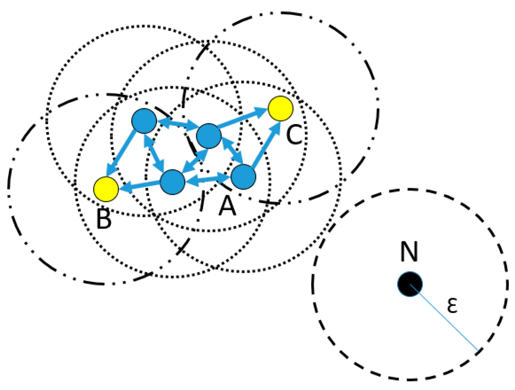
2.5. Density-Based Spatial Clustering of Applications with Noise (DBSCAN)

Density-based clustering algorithms are usual in the literature [43]. The best-known algorithm of this category is the Density-Based Spatial Clustering of Applications with Noise—DBSCAN [44]. The method can find clusters of an arbitrary shape, detecting them through high-density spheres and merging the nearby spheres forming clusters.

The DBSCAN uses a simple estimate of the minimum density level, based on a threshold for the number of neighbors, minPts, within the radius ε (with an arbitrary distance). Objects with more neighboring minPts within that radius (including the query point) are the central point.

The DBSCAN intends to find areas that satisfy this minimum density separated by lower density areas. For efficiency reasons, DBSCAN does not estimate density between points. Instead, all neighbors within the radius ε by a central point are considered part of the same cluster (known as direct attainable density). If any of these neighbors is chosen again as a central point, their neighborhoods will be included transitively (reachable density). Non-essential points in this set are called boundary points, and all points in the same set are connected to density. Points that are not accessible by density are considered noise and do not belong to any group [45].

Figure 2 illustrates the working principle of the DBSCAN and the elements. The minPts parameter is four, and the circles indicate the radius ε. Note that N is a noise point, A is a central point and, B and C are border points.

2.6. Self Organizing Maps (SOM)

Self-Organizing Maps (SOM) are artificial neural network architectures that are adjusted using unsupervised learning methods to cluster data sets, including missing values. They can be used to analyze and visualize complex multivariable data with multiple parameters [46].

The network presents advantages over other multivariate approaches because it can deal with nonlinearities in a system [47,48]. Because it can be elaborated using data without mechanical knowledge of the system, it can deal with noisy, irregular, or missing samples. In addition, it is easy to update and interpret information with many variables or parameters using visualization resources [49,50,51].

The SOM network is a matrix of M = m × m of artificial neurons. If these m² neurons are arranged in a grid or a plane, the network is called two-dimensional since it maps high-dimensional input vectors to a two-dimensional surface. For a given network, the input vector x = (x₁, x₂, …, x_n) has a fixed dimension n. These n components are connected to each neuron in the matrix. A synaptic weight w_ij is defined for connecting the i-th component of the input vector to the j-th neuron. Therefore, a n-dimensional vector w_j of synaptic weights is associated with each neuron j [52].

Equation (7) shows the function of the closest distance to the winning neuron j:

$$D_{min}\left(t\right)=\begin{array}{c}min\left\{D_i\left(t\right)\right\}\\ i\end{array}=\begin{array}{c}min\\ i\end{array}\left\{{\displaystyle \sum }_j{\left(x_j\left(t\right)-w_{ij}\left(t\right)\right)}^2\right\}$$

(7)

where w_ij are the weights at the initial iteration t = 0, which are small randomly generated values, t is the number of the current iteration, and x_j is a randomly selected vector from the training data set.

Equation (8) shows the update function of the winning weight vectors and their neighbors:

$$w_i\left(t+1\right)=w_i\left(t\right)+\alpha \left(t\right)\times \left(x-w_i\left(t\right)\right), \forall i \in N_j$$

(8)

where α(t) is the function of the learning rate that decreases exponentially with the iterations; it is calculated by Equation (9):

$$\alpha \left(t\right)={\alpha }_0{e}^{\frac{-t}{3T}}$$

(9)

where α₀ is the initial learning rate and T the number of iterations, both user-defined data.

In Equation (10), the neighborhood order function can be observed:

$$d\left(t\right)=\left[d_0{e}^{\frac{-t}{3T}}\right]$$

(10)

d₀ being the initial topological neighborhood.

2.7. Particle Swarm Optimization (PSO)

The Particle Swarm Optimization (PSO) algorithm is the most used, popular, and famous swarm-inspired method for optimization [10]. It was inspired by the social behavior of animals that behave with flock characteristics, simulating their collective intelligence [13,53]. Beyond the optimization applications with real data, PSO has been widely used in binary, combinatorial, and clustering optimization problems [9]. In optimization problems, positions represent a candidate solution to the current task. However, in clustering, this depends on the coding and parameters [25].

The learning process of the particles comes from two sources: their own experience, called cognitive learning, and the combined learning of the whole cluster (or a topological neighborhood) called social learning. The first case is represented by the best position of the particle (pBest) reached until the current iteration, and the best position represents social learning achieved considering, for example, the entire population (gBest). Together, cognitive and social learning are used to calculate the velocity of particles and their next position [13].

The most used encoding scheme for partial clustering considers a particle a complete candidate solution [10]. In this case, the agent contains the spatial coordinates of all n_k centroids concatenated in a vector. The PSO can be applied directly, using the position and velocity, according to Equations (11) and (12), respectively:

$$x_i\left(\mathrm{t}+1\right)=x_i\left(\mathrm{t}\right)+v_i\left(\mathrm{t}+1\right)$$

(11)

$$v_i\left(\mathrm{t}+1\right)=\omega \times v_i\left(\mathrm{t}\right)+q_1\times r_1\times \left(pBes{t}_i\left(\mathrm{t}\right)-x_i\left(\mathrm{t}\right)\right)+q_2\times r_2\times \left(gBest\left(\mathrm{t}\right)-x_i\left(\mathrm{t}\right)\right)$$

(12)

where ω is the inertia weight, x_i is the position of the particle, v_i is the speed, pBest_i is the best position ever found by each particle, gBest is the best position found by the group, q₁ and q₂ are two previously defined constants, and r₁ and r₂ are two numbers randomly generated in the interval [0, 1].

The algorithm is often initialized by randomly scattering particles over the search space. The same process generates the initial speeds, but they are initialized equal to zero in some other cases. The inertia weight ω is often less than one, and it is used to avoid divergence in the response. It is also common to limit the speed of the particles to an interval [−v_max; + v_max] [54].

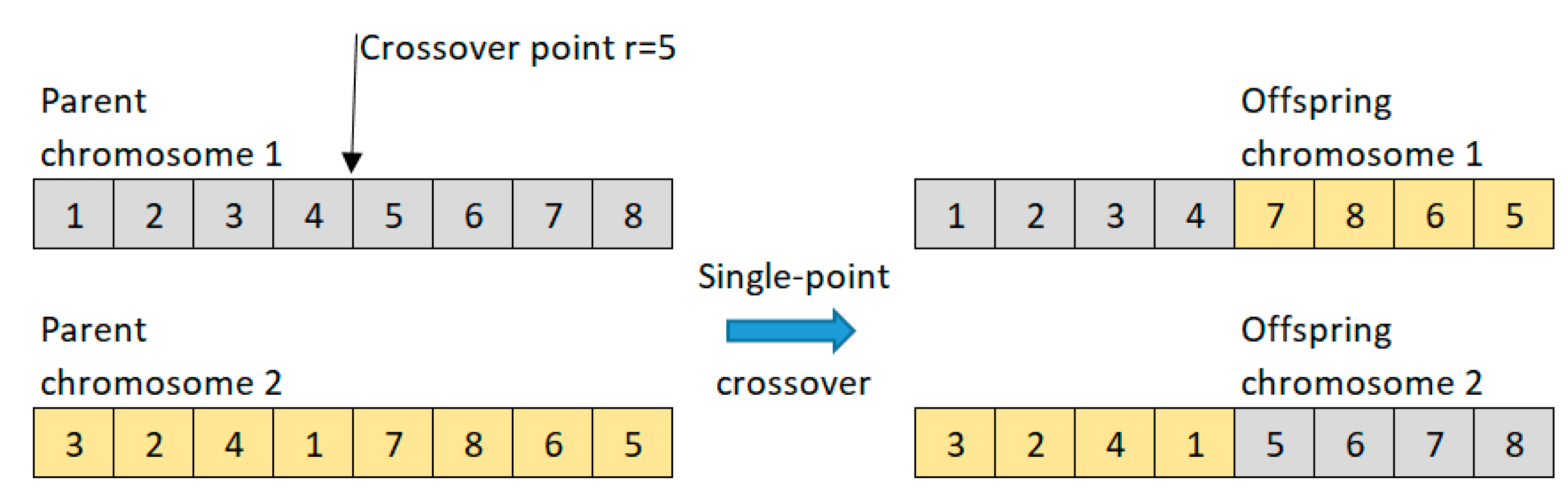
2.8. Genetic Algorithm (GA)

Evolutionary computing draws ideas from evolutionary biology to develop search and optimization techniques to solve complex problems. Evolutionary algorithms are rooted in the Darwinian Theory of the evolution of species. Darwin proposed that a population of individuals capable of reproducing is conditioned to (genetic) variation followed by natural selection results in new populations increasingly adapted to their environment. This proposal was very radical when it was first formalized at the end of the 1850s. It suggested that a simple reproduction process with variation and selection would be sufficient to produce complex life forms [54,55,56].

The Genetic Algorithm (GA) models genetic evolution, in which the characteristics of individuals are expressed using genotypes. The leading operators are selection (to model the survival of the fittest), recombination through the application of a crossover operator (to model reproduction), and mutation. The goal of the mutation is to introduce new genetic material into an individual, that is, to add diversity to the genetic characteristics of the population [57]. As in the PSO, an individual (chromosome or agent) presents a complete candidate solution for a given problem [58].

The chromosome based on gene configuration defines the genotypes. Each chromosome is evaluated by a cost function (fitness). A certain number of chromosomes were defined at the start parameter composes the first generation. Based on the optimization of the problem, the following generations are created based on selection, crossover, and mutation operators [59].

In the crossover, genes are exchanged on a specific chromosome, generating new individuals with another configuration. Figure 3 presents the classic one-point crossover [54,60].

Mutation operation corresponding to a spurious gene change after crossover, as illustrated in Figure 4.

2.9. Differential Evolution (DE)

Differential Evolution (DE) is another technique inspired by the evolution of species. In the literature, it has proved to be a viable candidate for optimization and clustering problems. In this case, agents are called vectors and are stochastically generated as in PSO and GA [61].

The positions of the vectors provide valuable information about the cost function scenario. As long as a good uniform randomization method is used to build the initial population, the initial agents provide a good representation of the entire search space, with relatively large distances between them. As the search progresses, the distances between the vectors decrease, with everyone converging on the same solution. The magnitude of the initial distances between individuals is influenced by the population size in an inversely proportional way [57].

In DE, a population of NP candidate solutions indicated as x_i,G, where i denotes each agent and G represents the generation of the population, is used. As in GA, the operators are crossover, mutation, and selection [62].

The optimization process starts with selecting a vector, named target vector, and three others were chosen at random: x_r1, x_r2, and x_r3. In the next step, the mutation operator is applied, generating a new donor vector v_i,G through Equation (13):

$$v_{i,G}=x_{r1,G}+F\times \left(x_{r3,G}+x_{r2,G}\right)$$

(13)

where F is a user-defined constant from [0, 2], and i = 1, …, NP, r₁, r₂, r₃ $\in$ {1, …, NP}.

Then, a crossover operator, also called recombination, incorporates successful solutions into the population. The trial vector u_i,G is created by the binomial combination of the target vector x_i,G and the donor vector v_i,G elements. Each element of the trial vector comes from x_i,G with crossover probability C_r $\in$ [0, 1] selected along with the population, as in Equation (14) [62]:

$$u_{j, i,G+1}=\{\begin{array}{c}{v}_{j,i,G+1} \mathrm{if} {\mathrm{rand}}_{\mathrm{i},\mathrm{j}}\left[0, 1\right]\le C_r \mathrm{or} \mathrm{if} \mathrm{j}=I_{rand}\\ x_{j,i,G+1} \mathrm{if} {\mathrm{rand}}_{\mathrm{i},\mathrm{j}}\left[0, 1\right]>C_r \mathrm{or} \mathrm{if} \mathrm{j}\ne I_{rand}\end{array}$$

(14)

Finally, the selection operator differs from GA. In this case, the target vector x_i,G is compared with the trial vector u_i,G, and the corresponding vector with the best fitness value is taken into next-generation, agreed approach, as in Equation (15):

$$x_{ i,G+1}=\{\begin{array}{c}{u}_{i,G+1} \mathrm{if} f\left(u_{i,G+1}\right)\le f\left(x_{i,G}\right) \mathrm{where} i=1,2,\dots N\\ x_{i,G} \mathrm{otherwise}\end{array}$$

(15)

3. Clustering Metrics

A critical step on the encoding success of clustering algorithms is the metrics that evaluate the quality of the formed groups, which are focused on similarity or dissimilarity distances. Towards this statement, it can be found that metrics focused on similarity optimize the cluster cohesion. On the other hand, methods that work with dissimilarity aim to present as much as possible more separate groups.

3.1. Sum of Squared Errors (SSE)

The Sum of Squared Errors (SSE) is a measure of group compaction. It is a minimization index since the smaller the value, the cluster is more compact [63,64,65].

Consider X = {x₁, x₂, …, x_n} as a dataset with n samples. Suppose that the samples in X present rigid labels belonging to clusters k without overlap, being K = {c₁, c₂, …, c_k} the centroids. The clustering algorithm seeks to find the ideal partition P = {P₁, P₂, …, P_m}, positioning the k centroids iteratively [61]. This metric can be defined by Equation (1) [10], being the same used as the objective function to the K-Means.:

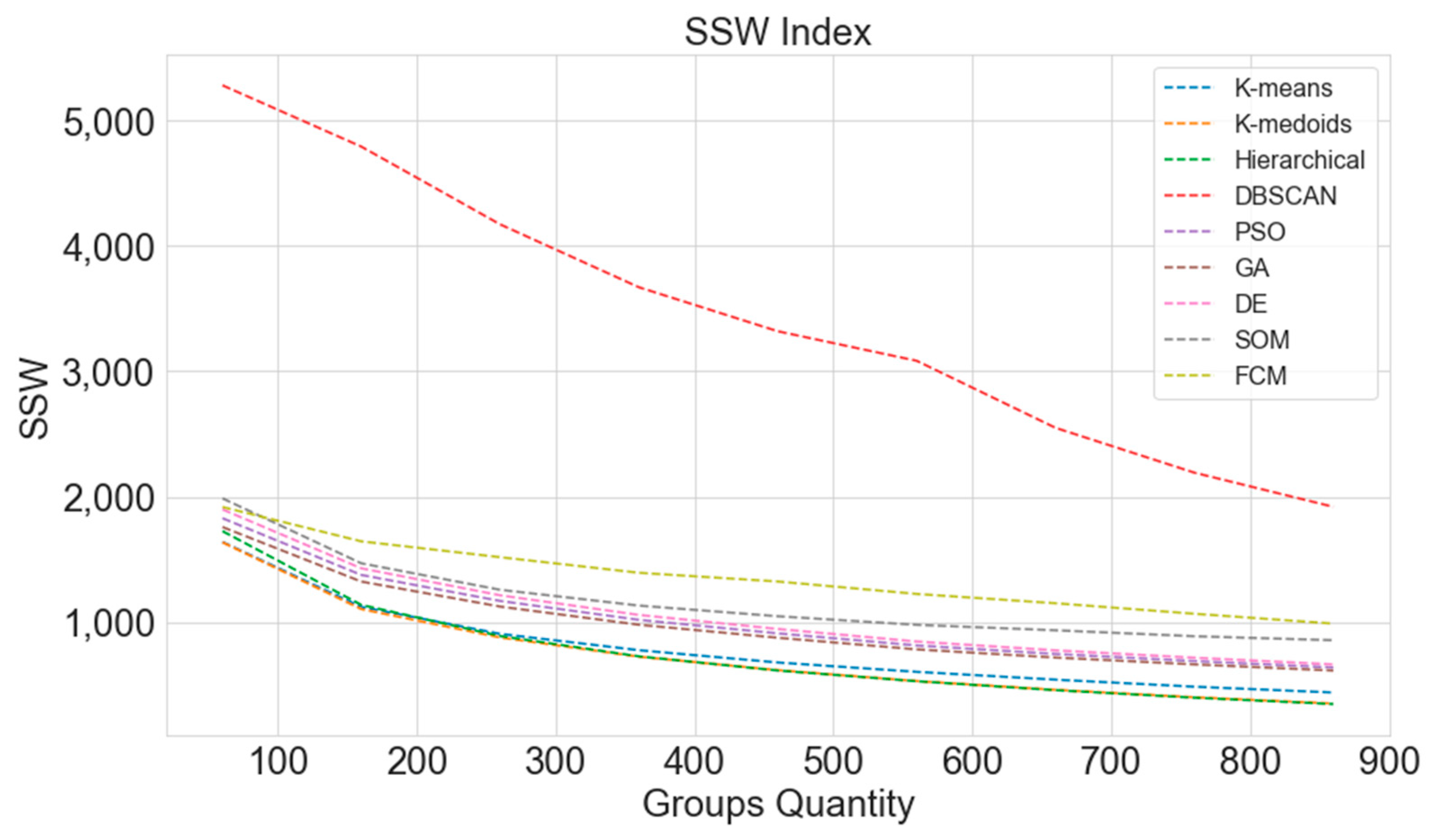
3.2. Sum of Squares within Clusters (SSW)

Sum of Squares Within Clusters (SSW) is a metric of group compaction and a minimization index. What sets it apart from the SSE is the non-square result of the summation equation [10,13,14]. This measure is dated by Equation (1), as showed in the previous Section 2.

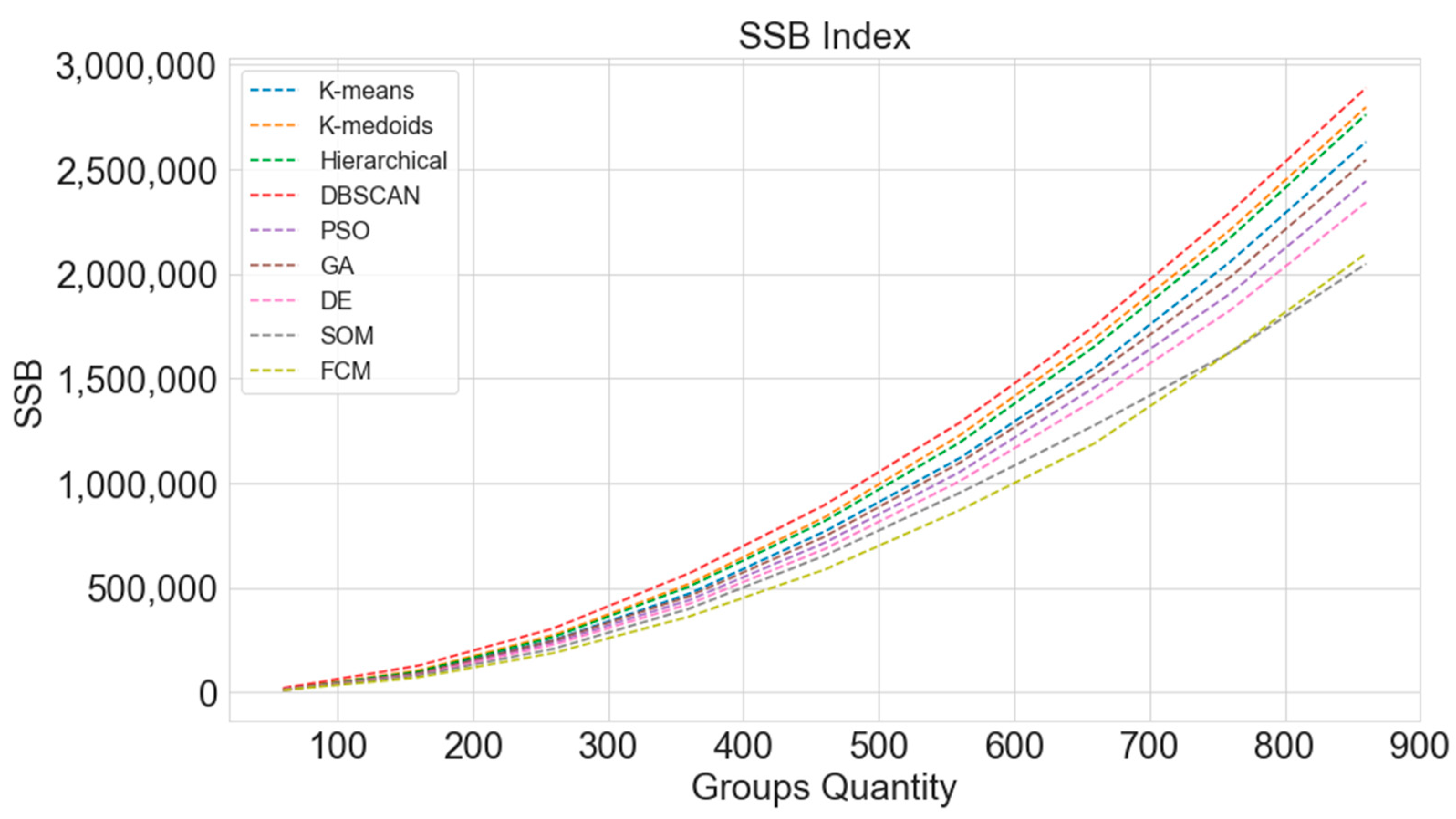
3.3. Sum of Squares between Clusters (SSB)

The Sum of Squares Between Clusters (SSB) measures how outlined the groups are. It is a maximization index. The higher the value, the more distinct the groups formed by the respective algorithms [66,67]. It is a criterion for measuring the separation of groups and can be calculated by Equation (16):

$$SSB=\frac{1}{2}{\displaystyle \sum }_{k=1,l=1,l\ne k}^{K}dist\left(c_l-c_k\right)$$

(16)

where c_k is the centroid of cluster k and c₁ are the other clusters [10].

3.4. Calinski-Harabasz Index (CH)

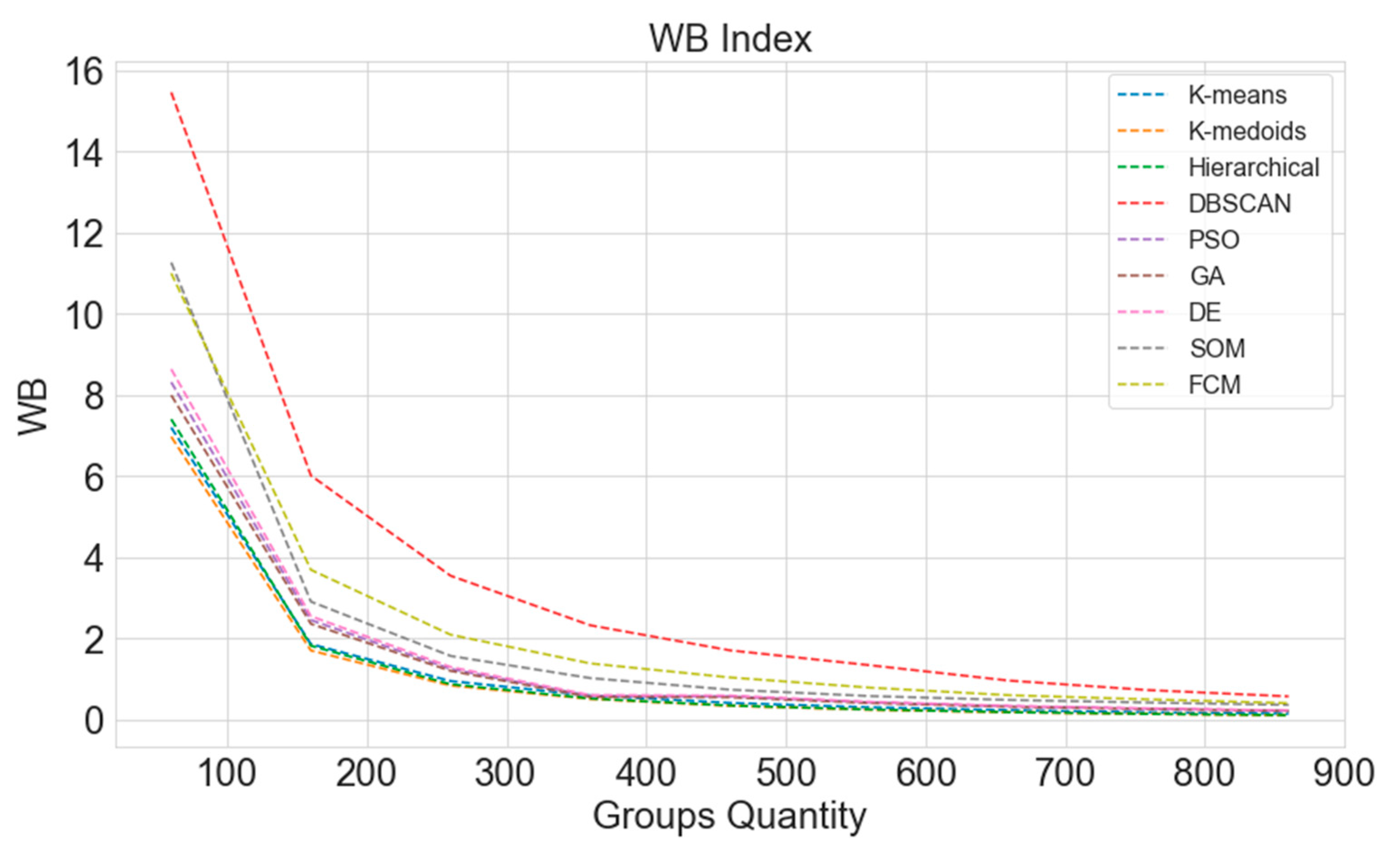
The Calinski-Harabasz index (CH) is a composition between the SSW and SSB, considering the number of centroids and the data. It is a maximization index [14,61,62,63]. Equation (17) shows the relationship of the elements exposed above:

$$CH=\frac{SSB/\left(k-1\right)}{SSW/\left(n-k\right)}$$

(17)

The CH metric creates a relationship between SSW, SSB, the total number of elements in the sample, and k, the number of centroids [67].

3.5. WB Index

The WB index is also a composition between the SSW and SSB indexes, adding a relationship between these metrics and the number of centroids. However, in this case, it uses only the number of centroids. It is a minimization metric [14,66,67,68].

Equation (18) presents the relation of the elements, as established by [67]:

$$WB=k\times SSW/SSB$$

(18)

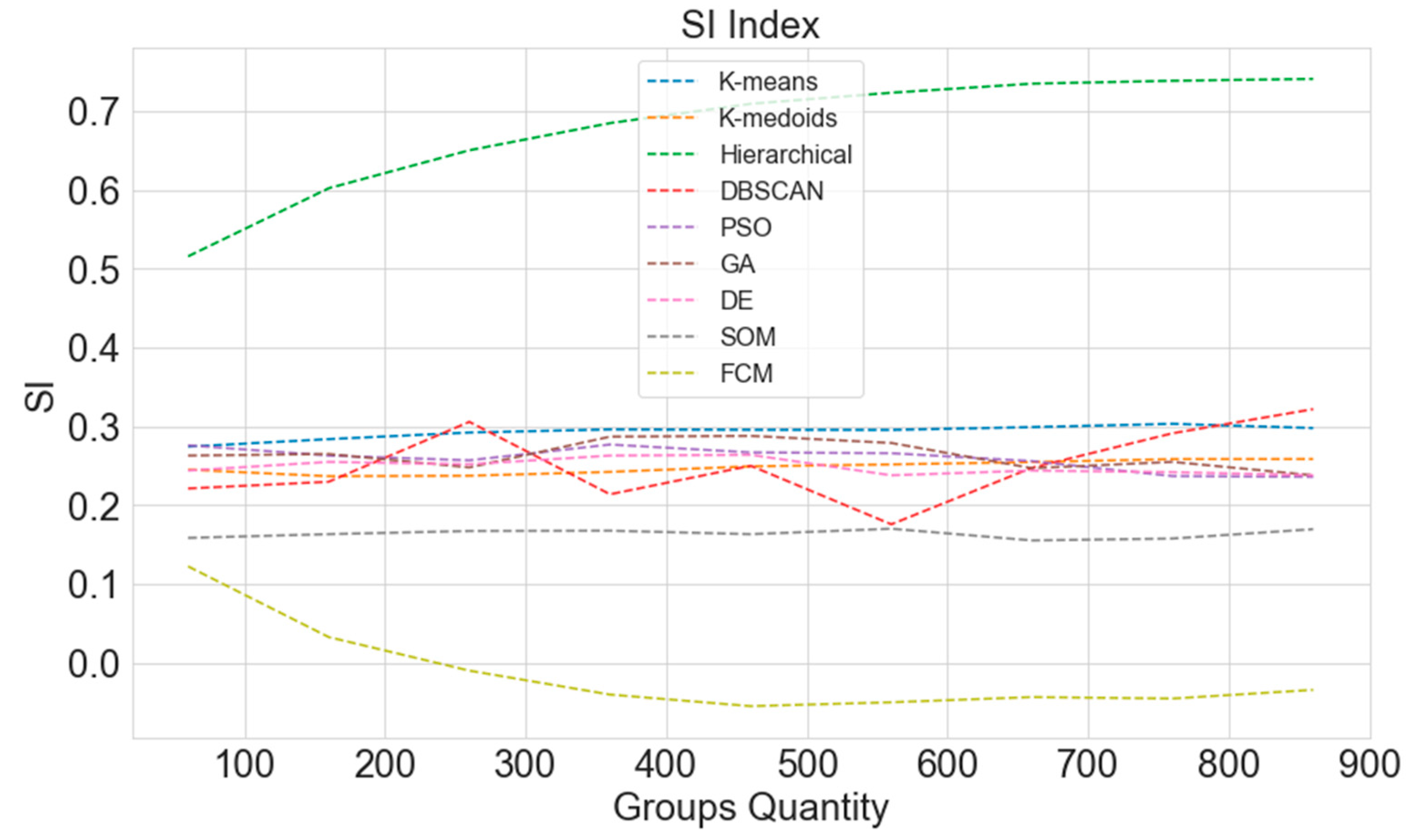
3.6. Silhouette Index (SI)

The Silhouette Index (SI) is a metric used to assess cluster validity. Its value can vary from (−1 < SI < 1). It measures how similar observed data is to other observations in its group compared to the samples allocated to the group closest to it. The SI values close to −1 indicate the data was erroneously entered in the target group, while values close to zero show the data could be in its target group as well as in some other group. SI values close to 1 indicate that the data are correctly allocated [10,69,70].

Equation (19) presents the formula for calculating the SI Index:

$$SI=\frac{1}{N}{\displaystyle \sum }_{i=1}^N\frac{b_i-a_i}{\max \left(b_i, a_i\right)}$$

(19)

where N is the number of clusters, and a_i is given by Equation (20):

$$a_i=\frac{1}{N_k}{\displaystyle \sum }_{x_j\in C_k}dist\left(x_i,x_j\right)$$

(20)

and N_k is the number of objects in a specific cluster, b_i is given by Equation (21):

$$b_i=mi{n}_{h\in \left\{1,\dots ,K\right\},h\ne k}\left(\frac{1}{N_h}{\displaystyle \sum }_{x_j\in C_h}dist\left(x_i,x_j\right)\right)$$

(21)

It means that $a_i$ is the mean distance between object i and all other data points in the same cluster, and $b_i$ is the minimum mean distance of object i to all points in any additional cluster h, of which this object does not belong.

4. Case Study, Results, and Discussions

This work was developed in an actual data set supplied by an automotive industry from Ponta Grossa-PR, Brazil, that cannot be nominated due to confidentiality aspects agreed between parts. There is an immediate need to expand the company’s focus to include the analysis of large sample sets. The best practice towards cost efficiency on the supply chain of components can be replicated, multidimensional and complex for manual analysis.

4.1. Industry Data

The data collection stage was initiated throughout a meeting with a multi-functional team of the company, including specialists from the following areas: manufacturing, engineering, product engineering, purchasing, quality, materials, logistics, production, and supplier development. In this event, the problem was discussed together with the business development team. The objective was grouping parts by similarity for future cost comparison, following the steps above:

Step 1—Load the complete SAP system database: at this step, the industry material planners identified all items by part number and checked by stock movements over the last three months. Note that just recently purchased parts with interest in cost analysis are included on the initial data set;

Step 2—Select continuous quantitative data: at this step, product engineering, manufacturing engineering, and accounting departments were invited to discuss the attributes of each part number downloaded. Therefore, clarifications on the nature of the data could be discussed for further classification considering quantitative and qualitative aspects. Observe that this case study only considers quantitative data;

Step 3—Eliminate components with missing data: some selected parts were incomplete. We highlight that most of the clustering does not work well with incomplete data. Therefore, part numbers with an incomplete data set were suppressed;

Step 4—Consider NCM (Mercosur Common Nomenclature) as the lower limit of the number of groups to be created: clustering techniques’ challenge is determining the number of clusters in advance. Based on this premise, several discussions with manufacturing and product engineering teams were carried out to identify the potential interval of dataset labels. The conclusion was that the NCM could be a good reference as lower limit (200) and engineering class number as the upper limit (621).

The first loading of systemic information raised 4267 items with 14 dimensions, among which the multi-functional team selected the following dimensions: Weight, Length, Width, Height, Volume, and Density. At the end of the 3rd step, 2765 parts were included in the database, which presented six dimensions for each sample.

As guided by the multi-functional team in the 4th and 5th steps, 200 different NCM codes and 621 different engineering class codes were used as a reference for defining the number of groups. With this background, it was expected that this study could show an ideal number of groups between 200 and 621.

For this reason, a search of the number of clusters was made with the following pre-established quantities: 60, 160, 260, 360, 460, 560, 660, 760, and 860, as most of the addressed algorithms requires the number of groups a priori. Values of 200 and 621 were purposely not included because manual analysis found inconsistencies in both cases.

4.2. Pre Processing Stages

Before the first run of the corresponding algorithms, it is necessary to perform a statistical exploration analysis of the data set. We noted some key points that interfere with the overall process quality of machine learning techniques as described below.

A logarithmic scaling resulting in the following weight data distribution in Figure 5 was applied to avoid a biased response.

This process was replicated to the remaining dimensions selected with similar results compared to the distribution before and after scaling.

Another point observed was that the corresponding dimensions presented a high numerical magnitude difference, and this implies a loss of significance to dimension with small magnitudes generating tendentious results. A normalization process known as z-score was applied to avoid this behavior, which is defined by Equation (22):

$$z_j=Z\left(x_j\right)=\frac{x_j-\overline{x_j}}{{\sigma }_j}$$

(22)

where x_j is the input data, $\overline{x_j}$ and ${\sigma }_j$ are the samples mean and the standard deviation of the j-th attribute, respectively. The transformed dimension presents a zero mean and a variance of 1.

The last preprocessing step used in this work was the PCA (Principal Component Analysis), a method based on the projection of data in a smaller subspace. This process aims at the possibility of reducing the number of dimensions while maintaining its significance in this projected subspace. Dimensional reduction techniques lessen the computational cost in multidimensional problems without harming the result due to preserving the importance of the original dimensions.

The well-known Iris dataset was used to validate the option for the PCA application. This dataset contains three labeled classes of flowers: Setosa, Versicolour, and Virginica, including 50 samples each, presenting four attributes: sepal length, sepal width, petal length, and petal width. Therefore, we consider the following scenarios:

(a)

Four dimensions sepal length, sepal width, petal length, and petal width without PCA application;

(b)

PCA application using only the first principal components;

(c)

PCA application using only the first and second principal components.

Then, we applied the nine clustering algorithms described in Section 3, generating

Table 1. Clustering algorithm performances considering the use of PCA on the Iris dataset.

Algorithm	(a)	(b)	(c)
GA	89.78%	92.00%	88.67%
FCM	89.78%	89.33%	91.33%
K-Medoids	89.78%	89.33%	91.33%
K-Means	89.78%	89.33%	91.33%
Hierarchical	89.78%	89.33%	90.00%
PSO	89.11%	90.00%	88.67%
DE	89.11%	90.00%	88.67%
SOM	85.33%	85.33%	85.33%
DBSCAN	67.78%	68.00%	67.33%

, which presents the percentage of correct classifications: for each scenario:

Note a slight variation from each of the scenarios chosen, which sustain the application of PCA to the Iris dataset. Indeed, in scenarios (b) and (c), the algorithms often overcame their performances considering the total number of dimensions.

After this validation, we applied the PCA to the automotive dataset. It was observed that each of the six principal components shows the following respective significances: 0.57, 0.18, 0.13, 0.09, 0.05, and 0. Note that the four first components present 95% of the energy of the signal.

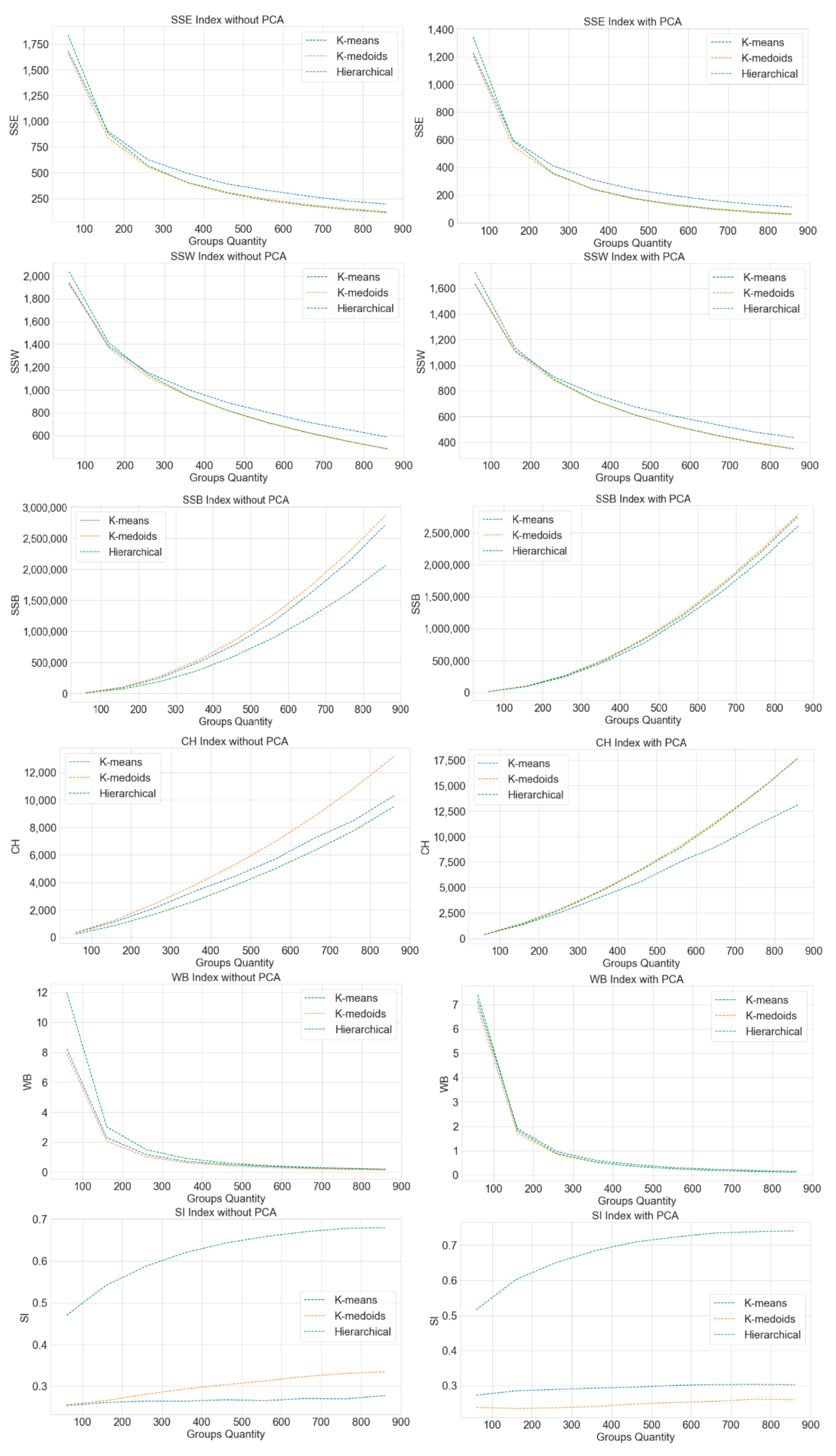
4.3. Computational Results

In this section, we present the results achieved by the nine algorithms described in Section 2 [71]. We present the results separated by an evaluation metric. For the stochastic methods, we present the best of 30 independent simulations.

Figure 6 presents the SSE index evolution throughout a different quantity of groups formed.

Graphical analysis shows a clear disadvantage of the DBSCAN algorithm. It is because of the input parameters, which cannot be translated as noise. For this purpose, even isolated data from the predefined radius must be considered as a group. Due to the distribution of the data in the dimensional space, many items fell into this situation. In the analysis of the groups, the large number of single items within several clusters generated by DBSCAN was precise.

It is possible to observe that the FCM algorithm did not perform better than the others. Again, this result can be attributed to the input data distribution, which caused the algorithm to fall to a local minimum, harming the result.

Another point to highlight is the positive result of the curves for the K-Medoids, Hierarchical, and K-Means algorithms with a distance from the other curves and the corresponding proximity.

In Figure 7 is plotted the SSW index.

In the same way as it was observed in the SSE, for the SSW index, there is a clear advantage to the K-Medoids, Hierarchical, and K-Means algorithms, and a disadvantage to the DBSCAN and FCM algorithms, for the reasons already discussed.

Figure 8 presents the results for the SSB index.

It is essential to point out that the SSB goal is to maximize the distance between centroids. This means that better distinct groups are formed, as the centroids are far apart.

The same reason explains the advantage of DBSCAN as the disadvantage found in the SSW for this algorithm. Many centroids ended up being formed with unique elements, which increased the sum of the Euclidean distances between the centroids of the groups included.

At the other end of the exact Figure, there is a disadvantage in the design of the groups formed in applying SOM and FCM algorithms. The performance highlights K-Medoids, Hierarchical, and K-Means.

Figure 9 presents the results for the CH index.

Remembering that the higher the CH, the better the quality of the clusters, or else, the more cohesive and outlined are the groups formed. This metric is calculated by Equation (18), representing a relationship between SSB, SSW, amount of data (n), and the number of centroids (k). In this way, equating the correlation at once to maximizes the SSB and minimizes the SSW. Once again, we observe the same tendency regarding the previous metrics.

Figure 10 shows the results for the WB index.

From Figure 10, we observe that the evolution curve of the WB index decreases significantly from the 360 groups formed for the different algorithms. This means that there is no significant reduction in the value of the index starting from this point. This index uses a ratio between SSW and SSB, which may indicate the groups’ formed quality, as much as the cohesion of the groups (SSW) and the distinction between the groups (SSB). Note that for the other metrics, this point is not easy to identify.

As mentioned, the multi-functional team of the company indicated the number of groups among the interval 200 to 621. The best performances were reached by the Hierarchical model, followed by K-Medoids and K-Means. Figure 11 shows the SI index.

Considering the Silhouette metric, the value is between [−1, 1], and the closer to 1, the more precise the formation of the groups. Then, we observe an advantage of the Hierarchical algorithm and a worse performance for FCM. The other algorithms have a more stabilized behavior concerning this metric, obtaining intermediate values. There is a significant difference in results and an inconclusive definition of the ideal number of centroids.

For each metric and algorithm application was checked an overall performance (

Table 2. Overall ranking using Borda count method considering different indexes and algorithm results.

Algorithm	SSE	SSW	SSB	WB	CH	SI	Total
Hierarchical	8	8	7	8	8	9	48
K-Medoids	9	9	8	9	9	3	47
K-Means	7	7	6	7	7	8	42
GA	6	6	5	6	6	7	36
PSO	5	5	4	5	5	6	30
DE	4	4	3	4	4	4	23
DBSCAN	1	1	9	1	1	5	18
SOM	3	3	2	3	3	2	16
FCM	2	2	1	2	2	1	10

), considering each result. The first place was awarded 9 points, the second 8, and so on, until the last place winner received 1 point.

On overall performance, the Hierarchal, was the general winner, slightly superior to K-Medoids, even though K-Medoids was the first in 4 of 6 different indexes when using the Borda count method [72]. It is an important finding since the literature strongly indicates that these classic methods tend to reach an inferior performance to more recent and sophisticated models, such as DBSCAN, FCM, and SOM. We also highlight that K-Medoids presented a lousy performance for SI, which led to a worse position in the ranking than the Hierarchical approach. Moreover, it seems to be clear that the advantages in their use are in the initialization and as actual data instead of a randomly generated centroid, as the ranking position of the K-Medoids is higher than the K-Means.

In this sense, we can resort to the no-free lunch theorem, since this investigation presents some particular premises, which are not usually addressed in the benchmark or other real-world problems. We expected that the FCM and SOM might achieve the best performances due to their complex clustering schemes. Once again, we can state that more than one algorithm should be used for clustering tasks.

The bio-inspired algorithm (GA, PSO, and DE) presented similar performances, highlighting the GA. Despite showing global search potential, they could not find the optimum global point in this study, and probably fell in local minimum points. Other bio-inspired approaches can be found in the literature, which can improve and expand the results reached in this investigation [73,74,75,76,77,78].

Another remark found in the literature is the computational cost regarding the hierarchical clustering method. We highlight that the Hierarchical approach is a deterministic one that does not depend on initialization. Therefore, a stochastic method like K-Medoids may request more aggregate computational effort, depending on the database, since it needs 30 independent runs.

It is essential to calculate multiple metrics, as only one might be insufficient to conclude the comparative analysis. It is also crucial since only one metric may not indicate the correct number of final clusters.

4.4. PCA Assessment for the Best Algorithms

The last analysis was performed to verify the influence of PCA on the results. The PCA potentially changes the classification based on the Borda count method (Table 2). In this sense, we ran the top 3 classified algorithms following the same premises of Section 4.3, considering the 6 original numerical dimensions, without PCA: K-Means, K-Medoids, and Hierarchical.

Figure 12 shows the values obtained for the same 6 indexes from Figure 6, Figure 7, Figure 8, Figure 9, Figure 10 and Figure 11, presenting the corresponding behavior before and after PCA application. On the right, we plot the same curves of the aforementioned figures, considering these 3 algorithms.

Initially, we highlight that the numerical values in the ordered axis are not comparable with and without PCA, since the number of dimensions is different, so the metrics’ values are also distinct.

For SSE, SSW, and SI, one can observe the same tendency in the curve, revealing that the use of PCA did not change the comparative performance. Considering the SSB, CH, and WB indexes, we noted that the Hierarchical method increased its performance, overcoming the K-Means with PCA, and presenting a close behavior regarding the K-Medoids.

In this regard, we elaborate a new ranking based on the Borda count method in

Table 3. Ranking using Borda count method considering results from Hierarchical, K-Means and K-Medoids with and without PCA application.

	Algorithm	SSE	SSW	SSB	WB	CH	SI	Total
With PCA	K-Medoids	3	3	3	3	3	1	16
	Hierarchical	2	2	2	2	2	3	13
	K-Means	1	1	1	1	1	2	7
Without PCA	K-Medoids	3	3	3	3	3	2	17
	Hierarchical	2	2	1	1	1	3	10
	K-Means	1	1	2	2	2	1	9

considering only Hierarchical, K-Means and K-Medoids:

Table 3 reveals the same tendency as Table 2. The K-Medoids and Hierarchical methods stood out, but the PCA favored the performance of the last. Due to the small number of contender algorithms, the lousy performance of K-Medoids and the outstanding performance of Hierarchical regarding the SI-index are barely visible. Because of this, the high number of wins achieved by the K-Medoids increased its position in the ranking. Therefore, it is likely that the ranking in Table 2 should not be much modified in the top positions with or without PCA, corroborating the findings presented in Section 4.2.

In general, it can be graphically verified that the influence of the PCA application does not interfere in the shape of the curve for the different indexes and algorithms despite slight ranking changes. Moreover, we noted a decrease in the average running time of K-Means and K-Medoids of around 2% and 8% regarding the Hierarchical algorithm. We advocate using PCA and more than one clustering method in real applications, especially for large datasets.

4.5. Company Feedback on Results

At the end of the computational step, with the clustering results, and after verifying the best performance of the Hierarchical, K-Medoids, and K-Means algorithms, the authors return to the automotive company to evaluate the findings. A meeting was held with the product engineering, manufacturing engineering, controllership, and purchasing teams to analyze the results critically. It was detected that three driver seats were in a cluster while the other was in a single group. When observing the original dataset, we found that the information in one of the dimensions of the single-seat was wrong, which led to a distortion in the results.

Other similar errors have been observed, mainly in small components whose basic geometric dimensions X, Y, and Z sometimes correspond to the packaging itself and not the actual dimensions of the part. In other cases, it was observed as a set of pieces and not as a single sample. A similar situation has occurred with the weight of the components. Once the data were corrected, the new groups formed were coherent.

Finally, we highlight that this investigation is a case study that tabulates results and displays a rank on the performance between 9 clustering algorithms considering six indexes primarily found in the literature. Although we are not introducing new or improved clustering techniques, clustering methods to identify price anomalies in an automaker is a relevant contribution to the field.

5. Conclusions and Future Work

In the automotive industry, it is widespread to develop new products with similar characteristics designed by different development teams, which increases the complexity of parts communization abroad for all products. Due to the high volume of data generated by multiple teams, that do not use data mining tools, this investigation can press the production cost by the supply chain increase of complexity. In this context, the present work used clustering tools to recognize the similarity between pieces of real databases provided by an automotive company. The goal was to optimize the costs of current products to identify opportunities and subsequent cost comparisons.

The techniques applied were K-Means, K-Medoids, Fuzzy C-Means (FCM), Hierarchical, Density-Based Spatial Clustering of Applications with Noise (DBSCAN), Self-Organizing Maps (SOM), Particle Swarm Optimization (PSO), Genetic Algorithm (GA), and Differential Evolution (DE). A ranking based on the Borda count method with the ordered performances indicated that the Hierarchical method stood out, slightly better than the K-Medoids and K-Means, due to a bad performance achieved by K-Medoids regarding SI-index. Despite those being considered classic approaches, they overcame the other methods regarding six clustering metrics.

This case study brings important practical contributions to the automotive industry, as it helps to recognize distortions between manufacturing costs, which optimizes the production process and leverages more competitive prices. It also improves the existing knowledge in the literature, helping to improve current techniques for the efficient allocation of automotive parts. One of them is the possibility of developing new methodologies for selecting automotive items with low cost and acceptable efficiency.

Despite the many tests performed by this work, the techniques consider only quantitative data, excluding qualitative information, such as item descriptions, NCM code, and engineering class, which is a limitation of the study. Thus, it is necessary to submit the database to models that simultaneously consider quantitative and qualitative information, such as Gower Distance.

A future study may be the application of other known techniques of data transformation, such as Box-Cox, to normalize the samples. This may increase the clustering capability of the models. Another possibility is the application of hybrid algorithm compositions that address various clustering techniques, seeking to eliminate the weak points of every single method. This area has shown interesting results in the literature. An example is the PSO-K, a hybrid between the PSO and K-means. The PSO finds an initial solution to reduce the undesirable initialization effects of the K-means. Finally, increasing the number of independent initializations beyond the 30 used in this study may lead the algorithms to better configurations.

References

1. Holtewert, P.; Bauernhansl, T. Optimal configuration of manufacturing cells for high flexibility and cost reduction by component substitution. Procedia CIRP 2016, 41, 111–116. [Google Scholar] [CrossRef]
2. Krappe, H.; Rogalski, S.; Sander, M. Challenges for handling flexibility in the change management process of manufacturing systems. In Proceedings of the 2006 IEEE International Conference on Automation Science and Engineering, Shanghai, China, 8–10 October 2006; pp. 551–557. [Google Scholar]
3. Argoneto, P.; Renna, P. Capacity sharing in a network of enterprises using the Gale–Shapley model. Int. J. Adv. Manuf. Technol. 2013, 69, 1907–1916. [Google Scholar] [CrossRef]
4. Hansen, J.O.; Kampker, A.; Triebs, J. Approaches for flexibility in the future automobile body shop: Results of a comprehensive cross-industry study. Procedia CIRP 2018, 72, 995–1002. [Google Scholar] [CrossRef]
5. Elmaraghy, H.A. Changeable and Reconfigurable Manufacturing Systems; Springer Science & Business Media: Berlin/Heidelberg, Germany, 2008. [Google Scholar]
6. Gameros, A.; Lowth, S.; Axinte, D.; Nagy-Sochacki, A.; Craig, O.; Siller, H. State-of-the-art in fixture systems for the manufacture and assembly of rigid components: A review. Int. J. Mach. Tools Manuf. 2017, 123, 1–21. [Google Scholar] [CrossRef]
7. Greska, W.; Franke, V.; Geiger, M. Classification problems in manufacturing of sheet metal parts. Comput. Ind. 1997, 33, 17–30. [Google Scholar] [CrossRef]
8. Flath, C.M.; Stein, N. Towards a data science toolbox for industrial analytics applications. Comput. Ind. 2018, 94, 16–25. [Google Scholar] [CrossRef]
9. Santos, P.; Macedo, M.; Figueiredo, E.; Santana, C.J.; Soares, F.; Siqueira, H.; Maciel, A.; Gokhale, A.; Bastos-Filho, C.J.A. Application of PSO-based clustering algorithms on educational databases. In Proceedings of the 2017 IEEE Latin American Conference on Computational Intelligence (LA-CCI 2017), Arequipa, Peru, 8–10 November 2017; pp. 1–6. [Google Scholar]
10. Figueiredo, E.; Macedo, M.; Siqueira, H.V.; Santana, C.J., Jr.; Gokhale, A.; Bastos-Filho, C.J. Swarm intelligence for clustering—A systematic review with new perspectives on data mining. Eng. Appl. Artif. Intell. 2019, 82, 313–329. [Google Scholar] [CrossRef]
11. Bang, S.H.; Ak, R.; Narayanan, A.; Lee, Y.T.; Cho, H. A survey on knowledge transfer for manufacturing data analytics. Comput. Ind. 2019, 104, 116–130. [Google Scholar] [CrossRef]
12. Cohen, S.; de Castro, L. Data clustering with particle swarms. In Proceedings of the 2006 IEEE International Conference on Evolutionary Computation, Vancouver, BC, Canada, 16–21 July 2006; pp. 1792–1798. [Google Scholar]
13. Alam, S.; Dobbie, G.; Koh, Y.S.; Riddle, P.; Rehman, S.U. Research on particle swarm optimization based clustering: A systematic review of literature and techniques. Swarm Evol. Comput. 2014, 17, 1–13. [Google Scholar] [CrossRef]
14. José-García, A.; Gómez-Flores, W. Automatic clustering using nature-inspired metaheuristics: A survey. Appl. Soft Comput. 2016, 41, 192–213. [Google Scholar] [CrossRef]
15. Pan, W.; Lu, W.F. A kinematics-aware part clustering approach for part integration using additive manufacturing. Robot. Comput. Manuf. 2021, 72, 102171. [Google Scholar] [CrossRef]
16. Zhong, X.; Xu, X.; Pan, B. A non-threshold consensus model based on the minimum cost and maximum consensus-increasing for multi-attribute large group decision-making. Inf. Fusion 2022, 77, 90–106. [Google Scholar] [CrossRef]
17. Kong, T.; Seong, K.; Song, K.; Lee, K. Two-mode modularity clustering of parts and activities for cell formation problems. Comput. Oper. Res. 2018, 100, 77–88. [Google Scholar] [CrossRef]
18. Bodendorf, F.; Merkl, P.; Franke, J. Intelligent cost estimation by machine learning in supply management: A structured literature review. Comput. Ind. Eng. 2021, 160, 107601. [Google Scholar] [CrossRef]
19. Chan, S.L.; Lu, Y.; Wang, Y. Data-driven cost estimation for additive manufacturing in cybermanufacturing. J. Manuf. Syst. 2018, 46, 115–126. [Google Scholar] [CrossRef]
20. De Abreu Batista, R.; Bagatini, D.D.; Frozza, R. Classificação automática de códigos NCM utilizando o algoritmo naïve bayes. iSys-Rev. Bras. Sist. Inf. 2018, 11, 4–29. [Google Scholar]
21. Macedo, L.C.L. Direito Tributário no Comércio Internacional; Edições Aduaneiras: Sao Paulo, Brazil, 2005. [Google Scholar]
22. Fattalla, F.C. Proposta de Metodologia Para Classificação Fiscal de Mercadorias Têxteis na Nomenclatura Comum do Mercosul. Doctoral Dissertation, Universidade de São Paulo, São Paulo, Brazil, 2016. [Google Scholar]
23. Pandove, D.; Goel, S.; Rani, R. Systematic review of clustering high-dimensional and large datasets. ACM Trans. Knowl. Discov. Data 2018, 12, 1–68. [Google Scholar] [CrossRef]
24. Hancer, E.; Karaboga, D. A comprehensive survey of traditional, merge-split and evolutionary approaches proposed for determination of cluster number. Swarm Evol. Comput. 2017, 32, 49–67. [Google Scholar] [CrossRef]
25. Nanda, S.J.; Panda, G. A Survey on Nature Inspired Metaheuristic Algorithms for Partitional Clustering. Swarm Evol. Comput. 2014, 16, 1–18. [Google Scholar] [CrossRef]
26. Yoo, Y. Data-driven fault detection process using correlation based clustering. Comput. Ind. 2020, 122, 103279. [Google Scholar] [CrossRef]
27. Xu, Z.; Dang, Y.; Zhang, Z.; Chen, J. Typical short-term remedy knowledge mining for product quality problem-solving based on bipartite graph clustering. Comput. Ind. 2020, 122, 103277. [Google Scholar] [CrossRef]
28. Dogan, A.; Birant, D. Machine learning and data mining in manufacturing. Expert Syst. Appl. 2021, 166, 114060. [Google Scholar] [CrossRef]
29. Mukhopadhyay, A.; Maulik, U.; Bandyopadhyay, S.; Coelho, C.A.C. Survey of multiobjective evolutionary algorithms for data mining: Part II. IEEE Trans. Evol. Comput. 2013, 18, 20–35. [Google Scholar] [CrossRef]
30. MacQueen, J. Some methods for classification and analysis of multivariate observations. In Proceedings of the Fifth Berkeley Symposium on Mathematical Statistics and Probability, Berkeley, CA, USA, 21 June–18 July 1965; Volume 1, pp. 281–297. [Google Scholar]
31. Park, H.-S.; Lee, J.-S.; Jun, C.-H. A K-means-like algorithm for K-medoids clustering and its performance. Proc. ICCIE 2006, 102–117. [Google Scholar]
32. Velmurugan, T.; Santhanam, T. Computational complexity between K-means and K-medoids clustering algorithms for normal and uniform distributions of data points. J. Comput. Sci. 2010, 6, 363. [Google Scholar] [CrossRef] [Green Version]
33. Mohd, W.M.B.W.; Beg, A.; Herawan, T.; Rabbi, K. An improved parameter less data clustering technique based on maximum distance of data and lioyd K-means algorithm. Procedia Technol. 2012, 1, 367–371. [Google Scholar] [CrossRef] [Green Version]
34. Sood, M.; Bansal, S. K-medoids clustering technique using bat algorithm. Int. J. Appl. Inf. Syst. 2013, 5, 20–22. [Google Scholar] [CrossRef]
35. Arora, P.; Varshney, S. Analysis of K-means and K-medoids algorithm for big data. Procedia Comput. Sci. 2016, 78, 507–512. [Google Scholar] [CrossRef] [Green Version]
36. Singh, S.S.; Chauhan, N.C. K-means v/s K-medoids: A comparative study. In Proceedings of the National Conference on Recent Trends in Engineering & Technology, Anand, India, 13–14 May 2011; Volume 13. [Google Scholar]
37. Zhao, R.; Gu, L.; Zhu, X. Combining fuzzy C-means clustering with fuzzy rough feature selection. Appl. Sci. 2019, 9, 679. [Google Scholar] [CrossRef] [Green Version]
38. Bezdek, J.C.; Ehrlich, R.; Full, W. FCM: The fuzzy C-means clustering algorithm. Comput. Geosci. 1984, 10, 191–203. [Google Scholar] [CrossRef]
39. Filho, T.S.; Pimentel, B.A.; Souza, R.; Oliveira, A. Hybrid methods for fuzzy clustering based on fuzzy c-means and improved particle swarm optimization. Expert Syst. Appl. 2015, 42, 6315–6328. [Google Scholar] [CrossRef]
40. Nguyen, H.; Bui, X.-N.; Tran, Q.-H.; Mai, N.-L. A new soft computing model for estimating and controlling blast-produced ground vibration based on hierarchical K-means clustering and cubist algorithms. Appl. Soft Comput. 2019, 77, 376–386. [Google Scholar] [CrossRef]
41. Alam, S.; Dobbie, G.; Rehman, S.U. Analysis of Particle Swarm Optimization Based Hierarchical Data Clustering Approaches. Swarm Evol. Comput. 2015, 25, 36–51. [Google Scholar] [CrossRef]
42. Anderberg, M.R. The broad view of cluster analysis. In Cluster Analysis for Applications; Elsevier: Amsterdam, The Netherlands, 1973; pp. 1–9. [Google Scholar]
43. Giacoumidis, E.; Lin, Y.; Jarajreh, M.; O’Duill, S.; McGuinness, K.; Whelan, P.F.; Barry, L.P. A blind nonlinearity compensator using DBSCAN clustering for coherent optical transmission systems. Appl. Sci. 2019, 9, 4398. [Google Scholar] [CrossRef] [Green Version]
44. Comesaña-Cebral, L.; Martínez-Sánchez, J.; Lorenzo, H.; Arias, P. Individual tree segmentation method based on mobile backpack LiDAR point clouds. Sensors 2021, 21, 6007. [Google Scholar] [CrossRef] [PubMed]
45. Ester, M.; Kriegel, H.P.; Sander, J.; Xu, X. A density-based algorithm for discovering clusters in large spatial databases with noise. In Proceedings of the 2nd International Conference on Knowledge Discovery and Data Mining KDD-96, Portland, OR, USA, 2–4 August 1996; pp. 226–231. [Google Scholar]
46. Abu-Mahfouz, I.; Banerjee, A.; Rahman, E. Evaluation of clustering techniques to predict surface roughness during turning of stainless-steel using vibration signals. Materials 2021, 14, 5050. [Google Scholar] [CrossRef]
47. Schubert, E.; Sander, J.; Ester, M.; Kriegel, H.P.; Xu, X. DBSCAN revisited, revisited: Why and how you should (still) use DBSCAN. ACM Trans. Database Syst. TODS 2017, 42, 1–21. [Google Scholar] [CrossRef]
48. Juntunen, P.; Liukkonen, M.; Lehtola, M.; Hiltunen, Y. Cluster analysis by self-organizing maps: An application to the modelling of water quality in a treatment process. Appl. Soft Comput. 2013, 13, 3191–3196. [Google Scholar] [CrossRef]
49. Alhoniemi, E.; Hollmén, J.; Simula, O.; Vesanto, J. Process monitoring and modeling using the self-organizing map. Integr. Comput. Eng. 1999, 6, 3–14. [Google Scholar] [CrossRef] [Green Version]
50. Kohonen, T. Overture. In Self-Organizing Neural Networks; Springer: Berlin/Heidelberg, Germany, 2002; pp. 1–12. [Google Scholar]
51. Hong, Y.-S.; Rosen, M.R. Intelligent characterisation and diagnosis of the groundwater quality in an urban fractured-rock aquifer using an artificial neural network. Urban Water 2001, 3, 193–204. [Google Scholar] [CrossRef]
52. Liukkonen, M.; Havia, E.; Leinonen, H.; Hiltunen, Y. Quality-oriented optimization of wave soldering process by using self-organizing maps. Appl. Soft Comput. 2011, 11, 214–220. [Google Scholar] [CrossRef]
53. Liukkonen, M.; Hiltunen, T.; Hälikkä, E. Modeling of the fluidized bed combustion process and NOx emissions using self-organizing maps: An application to the diagnosis of process states. Environ. Model. Softw. 2011, 26, 605–614. [Google Scholar] [CrossRef]
54. Ghaseminezhad, M.; Karami, A. A novel self-organizing map (SOM) neural network for discrete groups of data clustering. Appl. Soft Comput. 2011, 11, 3771–3778. [Google Scholar] [CrossRef]
55. Eberhart, R.; Kennedy, J. A new optimizer-using particle swarm theory. In Proceedings of the Sixth International Symposium on Micro Machine and Human Science, Nagoya, Japan, 4–6 October 1995; pp. 39–43. [Google Scholar]
56. De Castro, L.N. Fundamentals of Natural Computing: Basic Concepts, Algorithms, and Applications; CRC Press: Boca Raton, FL, USA, 2006. [Google Scholar]
57. Goldberg, D.E.; Holland, J.H. Genetic algorithms and machine learning. Mach. Learn. 1988, 3, 95–99. [Google Scholar] [CrossRef]
58. Booker, L.B.; Goldberg, D.E.; Holland, J.H. Classifier systems and genetic algorithms. Artif. Intell. 1989, 40, 235–282. [Google Scholar] [CrossRef]
59. Engelbrecht, A.P. Computational Intelligence: An Introduction; John Wiley & Sons: Hoboken, NJ, USA, 2007. [Google Scholar]
60. Zou, P.; Rajora, M.; Liang, S. Multimodal optimization of permutation flow-shop scheduling problems using a clustering-genetic-algorithm-based approach. Appl. Sci. 2021, 11, 3388. [Google Scholar] [CrossRef]
61. Mitchell, M. An Introduction to Genetic Algorithms; MIT Press: Cambridge, MA, USA, 1998. [Google Scholar]
62. Bhattacharjya, R.K. Introduction to Genetic Algorithms; Indian Institute of Technology Guwahati (IIT Guwahati): Guwahati, India, 2012; Volume 12. [Google Scholar]
63. Jayaprakash, S.; Nagarajan, M.D.; de Prado, R.P.; Subramanian, S.; Divakarachari, P.B. A systematic review of energy management strategies for resource allocation in the cloud: Clustering, optimization and machine learning. Energies 2021, 14, 5322. [Google Scholar] [CrossRef]
64. Lee, G.M.; Gao, X. A hybrid approach combining fuzzy C-means-based genetic algorithm and machine learning for predicting job cycle times for semiconductor manufacturing. Appl. Sci. 2021, 11, 7428. [Google Scholar] [CrossRef]
65. Senthilkumar, P.; Vanitha, N.S. A stride towards developing efficient approaches for data clustering based on evolutionary programming. Int. J. Emerg. Technol. Comput. Sci. Electron. 2013, 3, 27–32. [Google Scholar]
66. Ramadas, M.; Abraham, A.; Kumar, S. FSDE-forced strategy differential evolution used for data clustering. J. King Saud Univ.—Comput. Inf. Sci. 2019, 31, 52–61. [Google Scholar] [CrossRef]
67. Su, T.; Dy, J. A deterministic method for initializing K-means clustering. In Proceedings of the 16th IEEE International Conference on Tools with Artificial Intelligence, Boca Raton, FL, USA, 15–17 November 2005; pp. 784–786. [Google Scholar]
68. Thinsungnoena, T.; Kaoungkub, N.; Durongdumronchaib, P.; Kerdprasopb, K.; Kerdprasopb, N. The clustering validity with silhouette and sum of squared errors. In Proceedings of the International Conference on Industrial Application Engineering 2015, Kitakyushu, Japan, 28–31 March 2015. [Google Scholar] [CrossRef] [Green Version]
69. Fränti, P.; Sieranoja, S. K-means properties on six clustering benchmark datasets. Appl. Intell. 2018, 48, 4743–4759. [Google Scholar] [CrossRef]
70. Caliński, T.; Harabasz, J. A dendrite method for cluster analysis. In Communications in Statistics—Theory and Methods; Taylor & Francis: Abingdon, UK, 1974; pp. 1–27. [Google Scholar]
71. Rousseeuw, P.J. Silhouettes: A graphical aid to the interpretation and validation of cluster analysis. J. Comput. Appl. Math. 1987, 20, 53–65. [Google Scholar] [CrossRef] [Green Version]
72. Pérez-Medina, J.-L.; Villarreal, S.; Vanderdonckt, J. A gesture elicitation study of nose-based gestures. Sensors 2020, 20, 7118. [Google Scholar] [CrossRef] [PubMed]
73. Zhao, Q.; Xu, M.; Fränti, P. Sum-of-Squares Based Cluster Validity Index and Significance Analysis; Lecture Notes in Computer Science; Springer: Berlin/Heidelberg, Germany, 2009; pp. 313–322. [Google Scholar]
74. Ozturk, C.; Hancer, E.; Karaboga, D. Improved clustering criterion for image clustering with artificial bee colony algorithm. Pattern Anal. Appl. 2015, 18, 587–599. [Google Scholar] [CrossRef]
75. Kraiem, H.; Aymen, F.; Yahya, L.; Triviño, A.; Alharthi, M.; Ghoneim, S.S.M. A comparison between particle swarm and grey wolf optimization algorithms for improving the battery autonomy in a photovoltaic system. Appl. Sci. 2021, 11, 7732. [Google Scholar] [CrossRef]
76. Srinivas, T.; Madhusudhan, A.K.K.; Manohar, L.; Pushpagiri, N.M.S.; Ramanathan, K.C.; Janardhanan, M.; Nielsen, I. Valkyrie—Design and development of gaits for quadruped robot using particle swarm optimization. Appl. Sci. 2021, 11, 7458. [Google Scholar] [CrossRef]
77. Belotti, J.T.; Castanho, D.S.; Araujo, L.N.; Silva, L.V.; Antonini Alves, T.; Tadano, Y.S.; Stevan, S.L., Jr.; Correa, F.C.; Siqueira, H.V. Air pollution epidemiology: A simplified generalized linear model approach optimized by bio-inspired metaheuristics. Environ. Res. 2020, 191, 110106. [Google Scholar] [CrossRef]
78. Puchta, E.D.P.; Lucas, R.; Ferreira, F.R.V.; Siqueira, H.V.; Kaster, M.S. Gaussian adaptive PID control optimized via genetic algorithm applied to a step-down DC-DC converter. In Proceedings of the 12th IEEE International Conference on Industry Applications (INDUSCON), Curitiba, Brazil, 20–23 November 2016; pp. 1–6. [Google Scholar]
Figure 1. The final solution of the hierarchical clustering method showing a 2D dataset and corresponding dendrogram.
Applsci 11 09868 g001
Figure 2. Groups formed in the application of the DBSCAN algorithm with Min. Points = 4.
Applsci 11 09868 g002
Figure 3. Single-point crossover for a pair of chromosomes of length l = 8.
Applsci 11 09868 g003
Figure 4. Gene mutation of chromosomes with length l = 8.
Applsci 11 09868 g004
Figure 5. Weight distribution after logarithm scaling.
Applsci 11 09868 g005
Figure 6. SSE index evaluation over a different number of groups considering nine clustering methods.
Applsci 11 09868 g006
Figure 7. SSW index evaluation over different group amounts considering nine clustering methods.
Applsci 11 09868 g007
Figure 8. SSB index evaluation over different group amounts considering nine clustering methods.
Applsci 11 09868 g008
Figure 9. CH index evaluation over different group amounts considering nine clustering methods.
Applsci 11 09868 g009
Figure 10. WB index evaluation over different group amounts considering nine clustering methods.
Applsci 11 09868 g010
Figure 11. SI index evaluation over different group amounts considering nine clustering methods.
Applsci 11 09868 g011
Figure 12. Shape comparison before and after the application of PCA to each Index.
Applsci 11 09868 g012