Abstract
This work investigates an analysis method for the stability of a three-dimensional (3D) slope with weak zones considering spatial variability on the basis of two-phase random media and the finite element method. By controlling the volume fractions of rock and weak zones, two-phase random media are incorporated into the 3D slope model to simulate the random distribution of rock and weak zones. Then, a rotation of a Gaussian random field is performed to account for the inclination of the weak zones. The validity of the proposed model for use in the analysis of the stability of 3D slopes with weak zones was verified by comparing it to existing results and analytical solutions. The failure mechanism of the slope is considered by examining the plastic failure zone at incipient slope failure. The safety factor is sensitive to the inclination of the weak zones, but it is predictable. Parametric studies on the inclination of the layer of weak zones demonstrate that when the rotation angle of the weak zones is approximately parallel to the slope inclination, the slope is prone to slippage along the weak zones, resulting in a significant reduction in the safety factor. The findings of this research can serve as the foundation for further research on the stability of slopes with weak zones.
1. Introduction
The prediction and control of landslides caused by the instability of slopes with weak zones is of great practical significance in the risk assessment of earth disasters. Slope stability is closely related to the inclination, position and shape of the weak zones inside the slopes. Due to the strong degree of randomness in the spatial distribution of the weak zones within the slope, these factors are, to a certain extent, uncertain, so it is difficult to quantitatively evaluate the stability and failure consequences of the slope [1]. Stability analysis of slopes with weak zones is an essential element of safety design in practice.
The stability of a slope will be strongly affected by the distribution of its internal weak zones. For a slope composed of multiple zones, the damage is usually dominated by the spatial distribution of the weak zones [2]. To date, numerous approaches have been proposed to analyze the stability of slopes with weak zones, such as the rigid body limit equilibrium method, the model test method, and the finite element method [3,4,5,6,7,8,9,10,11].
However, natural rock and weak zones exhibit obvious spatial variability [12,13,14,15]. In some geotechnical engineering practices, due to long-term physical, chemical or geological effects, investigations that do not consider the spatial variability of rock and weak zones can lead to unconservative results [16]. The spatial variability of rock and weak zones can cause randomness and uncertainty in the distribution of weak zones inside the slope. Since the rock and weak zones of slopes are the products of a shared sedimentary history, structure and experience of human activities, the spatial distribution of the weak zones at a given site and the spatial distribution of the mechanical characteristics of the slope should have similar characteristics [17]. Therefore, random fields can be applied to simulate the non-homogeneity of the spatial distribution of weak zones.
Various investigations have been carried out on the effect of spatial randomness in rock and weak zones using the random field method [18,19,20,21,22,23,24,25,26]. However, most of these were limited to two-dimensional (2D) models. Li et al. [18] used representative slip surfaces together with Monte-Carlo simulation to conduct slope stability analysis. Li and Chu [20] developed a multiple response surface approach to perform slope reliability analysis. Qi and Li [23] explored the influence of the spatial variability of the strength parameter of weak zones on the critical slip surface of slopes using a 2D model. By comparison, research on three-dimensional (3D) slope stability remains less well documented [27,28]. Generally, compared with 2D models, 3D models have more degrees of freedom, and more computational effort is needed. Despite possessing the advantages of simplicity and computational efficiency, 2D models obviously deviate from reality. Furthermore, 2D analysis is likely to obtain conservative results compared with 3D analysis when performing deterministic slope stability analysis, but it cannot be ensured that the results of 2D analysis will be more conservative than 3D analysis when the spatial variability of weak zones parameters is considered [29,30]. These findings further illustrate that it is necessary to undertake 3D slope stability analysis in random weak zones and rock.
When investigating slopes with weak zones, the two-phase random media characterization method can be applied to soil–rock mixtures, since the overall material properties of the slope are dependent on the spatial distribution and volume fraction of the rock and weak zones. Griffiths et al. [31] simulated two-phase random media through the nonlinear translation of the Gaussian field, and combined the finite element method to characterize the spatial variability of rock and soil materials; Feng et al. [32] proposed a nonlinear transformation based on the Gaussian random field to realize the simulation of composite materials using two-phase random media. This was achieved by Fourier transform, improving the calculation efficiency. This method has high applicability for large-scale soil–rock mixture models and the characterizations of large numbers of model samples; Liu et al. [33] used two-phase random media to simulate the slope of soil–rock mixtures, and characterized the spatial variability of the soil [34] and rock layers of the weak zones, analyzing the failure mechanism of the soil–rock mixture slope with weak zones. A comparison of the slope stability analysis methods in the literature in presented in Table 1, including not only slope stability analysis, but also the analysis of the influence of weak zones on slope stability.

Table 1.
Summary of typical investigations on the analysis of slope stability.
This research aims to estimate the stability of a 3D corner slope with weak zones, introducing a two-phase random media model to invert the spatial distribution of rock and weak zones. Based on the basic theory of random fields, a mathematical theoretical model for characterizing rock weak zones using two-phase random media and a simulation method for the spatial inclination of weak zones are proposed. In this study, using the USDFILD platform in ABAQUS software, a Fortran program corresponding to the proposed model is developed, and 3D finite element modeling of slopes with weak zones is realized. The two-phase random media model and the finite element method are combined to quantitatively evaluate the safety factor of the slope, offering technical support for stability studies of slopes with weak zones.
2. Methodology
2.1. Method for Generating 3D Random Fields
The 3D random field is generated using the modified linear estimation method. The basic principle of this method is to generate a stationary Gaussian random field, where the mean is zero, and the unit variance and the spatial correlation length are √π [12]. Spatially correlated variables can be expressed by a linear equation combining fixed effects and random effects as follows:
where t represents the spatial variation of rock material properties at different locations, and fixed effects and random effects are represented by the mean value μ and the residual e, respectively. e is often assumed to be a constant, with deviations from this having a mean value u. The covariance matrix V of the residual e can be descirbed as follows:
where σ is the standard deviation of the random variable at each node, and C is the spatial autocorrelation matrix. To avoid generating negative values for the strength parameters of rock and weak zones, the strength parameters of some rock and weak zones usually adopt log-normal distribution. In this case, the random field can be modeled by the following method conversion:
where ε is the vector of correlated random variables; μln z is the mean of the logarithm of the material parameters; and σln z is the standard deviation of the logarithm of the rock property.
The modified linear estimation method needs to generate an n-dimensional m-vector attribute field with spatial cross-correlation matrix C. Then, vector attribute field stretch modeling is used to generate a random field with any specified spatial correlation length. The specific steps are as follows:
First, the n-dimensional space containing position vector s is discretized into n-dimensional grids with unit grid spacing. In addition, the grid nodes are filled using a random vector r with m random numbers following the standard Gaussian distribution.
Second, Cholesky decomposition is performed on the spatial cross-correlation matrix C according to Equation (4).
where L is the lower triangular matrix.
Third, calculate the position of y in s according to Equation (5).
where y is the attribute field containing the position vector; s is the random field containing the position vector; J is the direction vector and ε is a translation vector with n components. J and s are independent random variables, and they have specific values. In this study, the components of J and ε are uniformly distributed in the range of [0, π/2] and [0,1], respectively. According to Equation (2), the attribute field y will be rotated and translated to obtain the random field s.
Finally, the continuous attribute field of any coordinates can be calculated by Equation (6), as shown below.
where and are the jth component of the attribute field containing the position vector y and the ith node of element k, respectively; is a form function with 2n nodal elements, which is taken from the library of form functions established by the finite element method.
2.2. Method of Generating 3D Random Field
The stabilities of slope projects are strongly affected by the distribution of its internal weak zones. In the destruction of a slope composed of multiple zones, landslides are usually dominated by the spatial distribution of the weak zones. However, due to the constraints of project budget and construction schedules, it is almost impossible to obtain a complete distribution of zones within the slope through on-site surveys. In typical slope projects, only limited survey work is carried out. Therefore, the distribution characteristics of weak zones are only known in the survey operation area, and such information cannot be obtained at other locations.
The spatial distribution of weak zones at the same site and the spatial distribution of the mechanical characteristics of the rock and weak zones should have similar characteristics. In the random field, the spatial correlation of the layer of weak zones in the layer of weak zones between the two-slope rock and weak zones elements can be expressed using the square exponential autocorrelation function R(x, y, z), as shown below:
where R (x, y, z) represents the spatial correlation of the material unit; θx, θy and θz are the correlation lengths along x, y and z directions, respectively.
In this study, the anisotropic random field is used to characterize the inhomogeneity of the spatial distribution of the weak zones. When the spatial correlation of each unit in the simulated weak zone is relatively high, it can be regarded as the same weak zone. In addition, since the weak zones are usually continuously layered inside the slope, the simulation results obtained using this method are closer to the ground truth.
For a 3D stationary Gaussian random field, a two-phase random media can be reconstructed for the rock and weak zones using the following formula:
where is the random media of weak zones and rock; and is the volume fraction of weak zones. Reconstructions of typical weak zones and rock random media are shown in Figure 1, where 0 represents the volume fraction of weak zones, and 1 represents the volume fraction of rock [33].
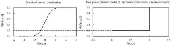
Figure 1.
Reconstructions of two-phase random media on the basis of the volume fraction of weak zones and rock.
The two-phase random media simulation method based on Gaussian random field is adopted in this research. This method can flexibly control the shape and orientation of the weak zone of the slope according to the actual geological survey situation, and can truly reflect the random distribution characteristics of the layer of weak zones in the slope. On the basis of the reconstruction of the typical two-phase random media shown in Figure 1, two typical samples of the two-phase random media are generated according to Equation (8), as shown in Figure 2, where the volume fraction of the weak zones is as assumed to be 20%.
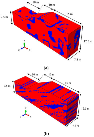
Figure 2.
Schematic diagram of the distribution of weak zones (red represents rocks, blue represents weak zones). (a) Typical sample of slope with homogenous weak zones (correlation length along all directions is 5 m); (b) typical sample of slope with layered weak zones (correlation length along x directions is 20 m; correlation length along y direction is 5 m; correlation length along z direction is 1000 m).
2.3. Method for Characterization of Anisotropic Correlation Structure
To make the simulation more similar to the actual slope, a 3D model was established, taking into account rotational anisotropy. The coordinates of the Gaussian random field were rotated around the X-axis in accordance with the given inclination angle. The rotation process can be expressed as in Equation (9).
where x’, y’ and z’ are the corresponding coordinates of x, y and z after rotation of the α angle about the X-axis. The distance after rotation can be obtained using Equations (10)–(12), as shown below.
The expression of the squared exponential autocorrelation function of rotational anisotropy can be obtained as:
Figure 3 illustrates the rotationally anisotropic after rotation of the α angle about the X-axis, the transversely anisotropic weak zone structure, and the correlation lengths. It can be clearly found from the figure that transverse anisotropy is a special case of rotational anisotropy. In addition, the autocorrelation function can well characterize the weak zones inside the slope.
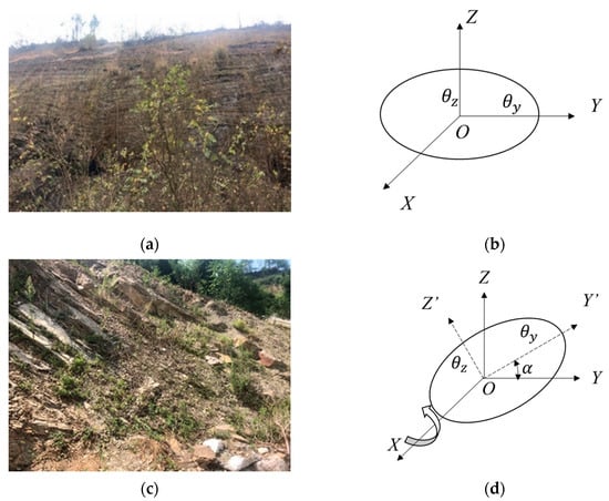
Figure 3.
Correlation structure of different related structures. (a) Horizontal rock slope; (b) schematic diagram of the correlation length of the x = 0; (c) rotational anisotropic slope; (d) correlation length of rotational anisotropy after rotation of the α angle about the X-axis.
For rotated anisotropy around the Y-axis, the correlation distance after rotation can be obtained using Equations (14)–(16), as shown below.
The expression of the squared exponential autocorrelation function of rotational anisotropy can be obtained as:
Figure 4 illustrates the rotationally anisotropic after rotation of α angle about the Y-axis, the transversely anisotropic weak zone structure, and the corresponding correlation lengths.
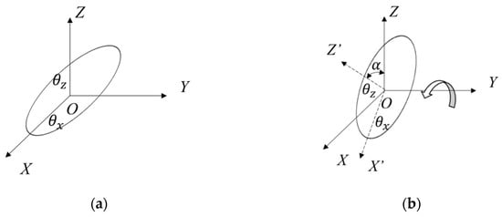
Figure 4.
Correlation distance of different related structures. (a) Schematic diagram of the correlation length of y = 0; (b) correlation length of rotational anisotropy after rotation of the α angle about the Y-axis.
For rotated anisotropy around the Z-axis, the correlation distance after rotation can be obtained by Equations (18)–(20), as shown below.
The expression of the squared exponential autocorrelation function of rotational anisotropy can be obtained as:
Figure 5 illustrates the rotationally anisotropic after rotation of α angle about the Z-axis, the transversely anisotropic weak zone structure, and the corresponding correlation lengths.
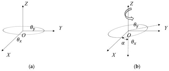
Figure 5.
Correlation distance of different related structures. (a) Schematic diagram of the correlation length of z = 0; (b) correlation length of rotational anisotropy after rotation of the α angle about the Z-axis.
On the basis of the above method, it is possible to characterize the slope where the weak zones are rotated by 0–60° around the X, Y, and Z-axes, respectively. Taking the soil volume fraction of the weak zones as 20%, the two-phase random media B (x, y, z) of the slope were generated, and the soil layer of the weak zones with different inclination angles was inverted. Some simulated samples of the slope are shown in Figure 6.
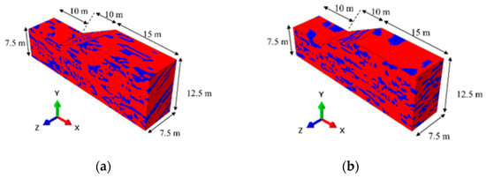
Figure 6.
Schematic diagram of the distribution of weak zones with different inclination angles. (a) Rotation angle of 30° around the X-axis; (b) rotation angle of 0.
2.4. Simulation and Model Verification of Weak Zones in Slopes
Taking into account the high degree of randomness the parameters such as shape, inclination angle, and the position of the weak zones, in order to perform verification, we used the Monte-Carlo simulation method to statistically analyze the results, generating a large number of random field samples through the modified linear estimation method. The airport was mapped to a finite element grid in order to construct a 3D model of a slope with weak zones. The stability of each slope in 100 examples of Monte-Carlo simulation was calculated. The safety factor was evaluated and compared with the content of the previous research [33] (Liu et al., 2018) for purposes of verification. As shown in Figure 7, the specific steps of combining USDFLD subroutine random field with the software Abaqus were as follows:
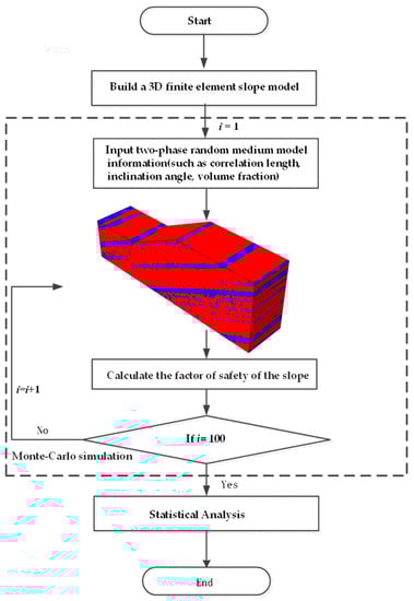
Figure 7.
Flow chart of the stability analysis of slopes with weak zones.
- (1)
- Use Abaqus to build a 3D finite element slope model, including defining the material parameters of the rocks and weak zones, and setting the grid and boundary conditions of the model in the analysis step. Then output an inp file (a file executed by the Abaqus software).
- (2)
- Associate the yield strength in the material parameters of the slope with the user-defined field variable User Defined Field, and set the state variable Depvar at the same time.
- (3)
- Call the random field generated by the USDFLD subroutine to replace the yield strength in the original slope model.
- (4)
- Carry out the stability calculation of the slope model with weak zones constructed in (3), and obtain the safety factor of the slope model.
- (5)
- According to the above steps, perform 100 Monte-Carlo simulations on the established model, and perform statistical analysis on the calculation results.
To verify the rationality of the two-phase random media characterization method, a typical 3D slope was established as shown in Figure 8. The model contains 213,240 C3D8 elements, and two-phase random media was used to characterize the weak zone and rock mass (using the ideal elastoplastic model); the two-dimensional slope model corresponding to the 3D model was in agreement with the content found in the literature, and the boundary conditions of the 3D model were consistent with the two-dimensional slope model found in the literature [33]. The material parameters used in this section are shown in Table 2.
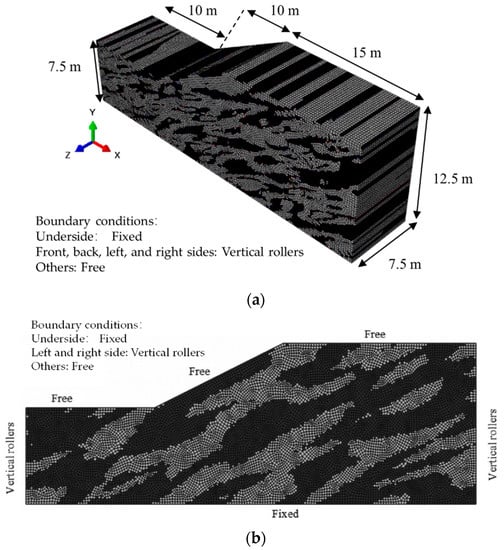
Figure 8.
A typical realization of two-phase random media for a slope with a weak zone fraction equal to 0.5 (the black area represents weak zones, and the gray area represents rock). (a) Schematic diagram of a typical 3D slope with weak zones (3D model used in this research); (b) schematic diagram of a typical two-dimensional slope with weak zones.
Table 2.
Material mechanical parameters of the validation slope model.
On the basis of the parameters shown in Table 2, a Monte-Carlo simulation (100 times) of the model in Figure 8 was performed, and the results obtained for the average safety factor are shown in Figure 9. When the volume fraction of the weak zones was 50%, the safety factor of the 3D model was 1.3% higher than that of the two-dimensional model (Liu et al., 2018) [33]. Considering that the number of Monte-Carlo is 100, the deviation of the mean is basically within the acceptable range. Compared with existing results, it can be verified that the 3D slope method representing the weak zones on the basis of two-phase random media is reasonable. Meanwhile, due to the spatial variability of the material parameters of the slope with weak zones, there is no straightforward rule for the failure mode of the slope and the irregular critical slip surface. The results obtained in this study suggest that the characterization of a 3D slope with weak zones on the basis of two-phase random media, combined with the finite element method, is able to automatically locate the critical slip surface where the internal strength of the slope is insufficient to resist the shear stress.
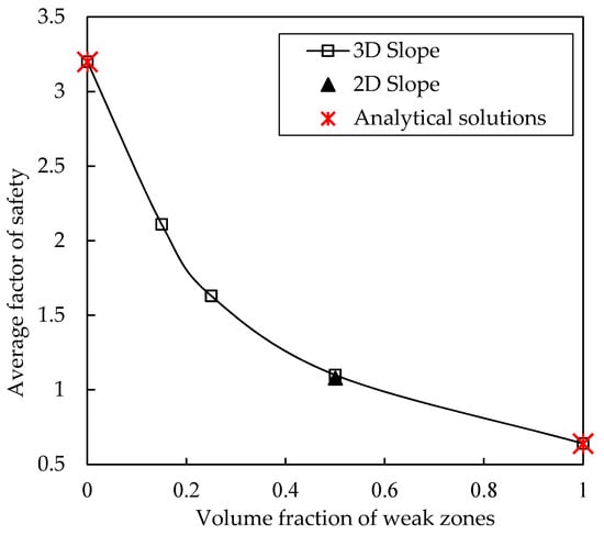
Figure 9.
Validation of proposed method by considering a rock-soil slope stability problem.
At the same time, it can be seen from Figure 9 that when the slope contains weak zones, the safety factor is 0.64, and when the slope is composed of rocks, the safety factor is 3.2 (the simulation results are consistent with the analytical solution). The median safety factor of slopes with weak zones and rocks is 1.92, which is greater than the safety factor of 1.14 obtained when the volume fraction of weak zones is 50%, meaning that the failure mechanism of slopes with weak zones may be dominated by weak zones. To study the failure principle of slopes with weak zones, Figure 10 shows the plastic strain diagrams of homogeneous slopes and slopes with weak zones. It can be seen from the figure that the homogeneous slope forms an obvious overall shear failure zone. In the slope with weak zones, due to the existence of the weak zones, a series of small shear failure zones appear in the failure mode of the slope along the laminar tendency. These small plastic strain regions reduce the safety factor of the slope.
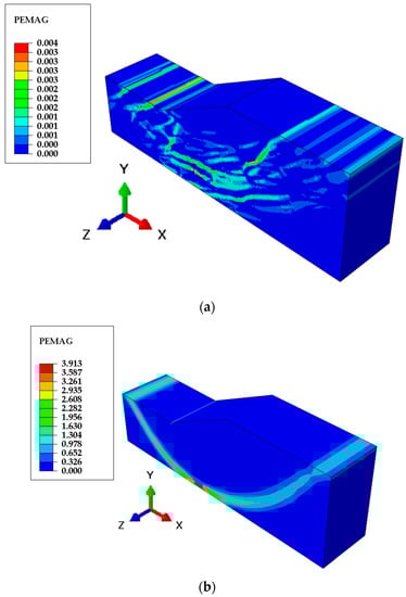
Figure 10.
Schematic diagram of typical failure modes of slopes. (a) Plastic strain diagram of the slope with weak zones; (b) homogeneous slope plastic strain diagram.
3. Slope Stability Analysis
Taking the Gangtou tunnel slope as the object of analysis, as shown in Figure 11, the position and shape of each section of the slope are quite different, and the distribution of weak zones inside the slope has spatial variability. The traditional two-dimensional model can only represent the rotation angle of the layer of weak zones of the weak zones in a certain section. However, it cannot reflect the real spatial distribution of the weak zones inside the slope.
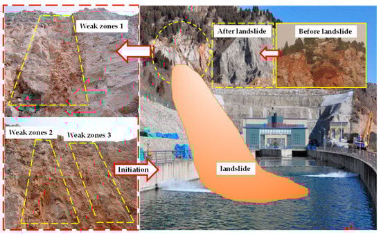
Figure 11.
Typical failure mode of Gangtou tunnel slope engineering (the rock in the slope is weathered flint-striped dolomite, and the soil in the weak zones is residual cohesive soil).
To illustrate the influence of the rotation angle of the layer of weak zones inside the slope on the stability and failure mechanism of the slope, weak zones with a rotation of 0–60° relative to the X-axis, Y-axis and Z-axis were generated in the 3D slope. The model was about 34 m long, 33 m high and 49 m wide. The number of finite element mesh elements was 399,611 and the number of nodes was 73669. The constraint boundaries around the model were normal bearing constraints, and the bottom of the slope was a complete constraint condition as is shown in Figure 12. Both weak zones and weathered flint strips dolomite are elastoplastic materials, and the Mohr-Coulomb yield criterion was adopted. The rock in the slope shown in Figure 11 is weathered flint-striped dolomite, and the soil in the weak zones is residual cohesive soil. The parameters are shown in Table 3.
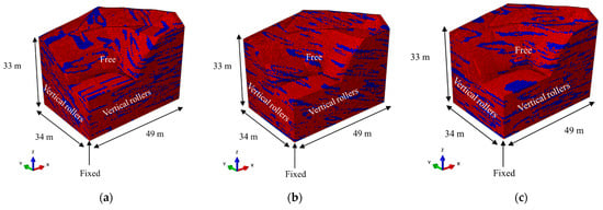
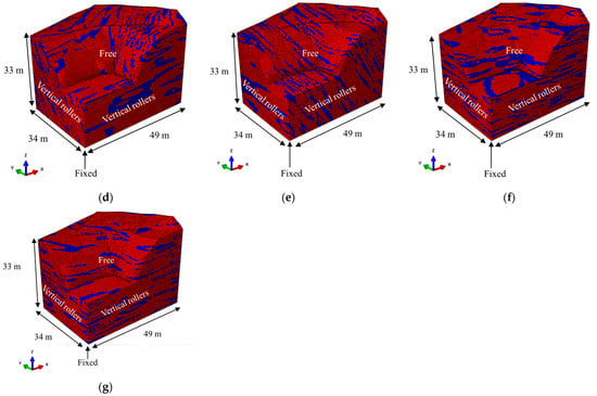
Figure 12.
Schematic diagram of the distribution of weak zones (red zone represents weathered flint strips dolomite; blue zone represents weak zones). (a) Rotation angle of 30° around the X-axis; (b) rotation angle of 30° around the Y-axis; (c) rotation angle of 30° around the Z-axis; (d) rotation angle of 60° around the X-axis; (e) rotation angle of 60° around the Y-axis; (f) rotation angle of 60° around the Z-axis; (g) Rotation angle of 0°.
Table 3.
Material mechanical parameters of the slope.
4. Results and Discussion
The stability calculation of the slope is shown in Figure 13. The rotation angle of the weak zone layer inside the slope is one of the main controlling factors for the safety factor of the slope. In the figure, when the weak zone is rotated 50° around the X-axis and 40° around the Y-axis, the slope and the inclination of the weak zone are approximately parallel, while simultaneously resulting in the safety factor of the slope being greatly reduced. Therefore, when the inclination of the weak zone is approximately balanced with the slope, the safety factor of the slope will decrease, and the slope is more prone to landslides.
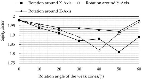
Figure 13.
FOS under different rotational angles of the weak zones.
The plastic strain diagram of the slope is shown in Figure 14, Figure 15 and Figure 16. It can be seen from the figures that when the slope is in a limit equilibrium state, yield occurs first at the weak zones, and the deformation of the weak zones develops continuously, resulting in an increase in the plastic zone. Therefore, when the weak zone layer is rotated at an angle of 50° around the X-axis and a rotation angle of 40° around the Y-axis, the safety factor of the slope reaches its lowest value. The figures suggest that the maximum plastic strain zone is likely to be parallel with the slope and the weak structural surfaces, thus decreasing the stability of the slope.
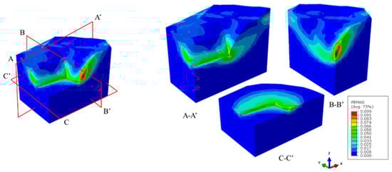
Figure 14.
Plastic strain diagram of the slope with transverse anisotropy of the weak zones (FOS = 1.98).
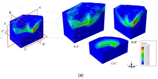
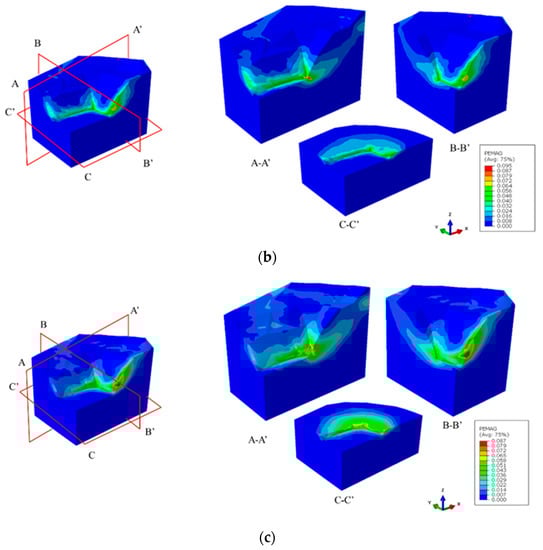
Figure 15.
Plastic strain diagram of the slope with 30° rotation angle of the weak zones. (a) Rotation angle of 30° around the X-axis (FOS = 1.87); (b) rotation angle of 30° around the Y-axis (FOS = 1.89); (c) rotation angle of 30° around the Z-axis (FOS = 1.94).
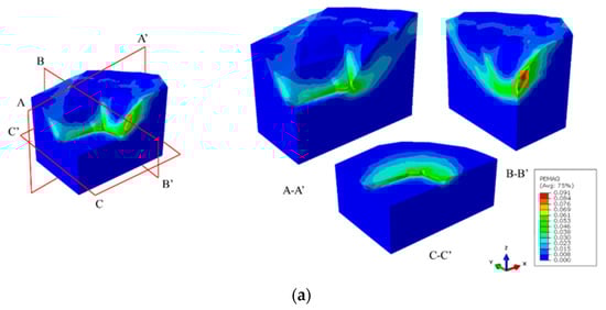
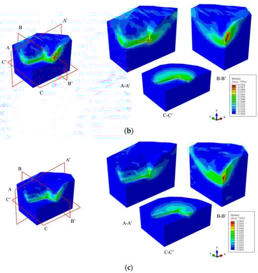
Figure 16.
Plastic strain diagram of the slope with 60° rotation angle of the weak zones. (a) The rotation angle of 60° around the X-axis (FOS = 1.89); (b) the rotation angle of 60° around the Y-axis (FOS = 1.97); (c) the rotation angle of 60° around the Z-axis (FOS = 1.98).
5. Conclusions
Aiming at the uneven spatial distribution of weak zones in slopes, this work investigated a mathematical theoretical model based on two-phase random media to characterize a 3D slope with weak zones. Based on the USDFILD platform in ABAQUS software, a Fortran program corresponding to the proposed model was developed, and the 3D finite element modeling of the slope with weak zones was performed. By setting the coordinate rotation angle of the anisotropic correlation structure, the inclination angle of the weak zones in the slope model was controlled. The validity of the proposed model for the analysis of the stability of 3D slopes with weak zones was verified on the basis of existing research results and analytical solutions. At the same time, the calculation results show that the above-mentioned characterization method combined with the finite element method is able to realize the automatic retrieval of the internal slip surface of the slope. By inverting the failure mode of the slope with weak zones, it can be found that the stabilities of slopes with weak zones re dominated by those weak zones.
Taking the Gangtou tunnel slope as the object of study, a stability analysis of a 3D slope with weak zones was carried out, and the influence of the inclination angle of the weak zones on the slope stability was analyzed using the 3D finite element model. The results show that the weak zones weaken the strength of the slope, leading to a decrease in safety factor. When the inclination angle of the weak zones was approximately parallel to the slope angle, the slope with the weak zones was more prone to instability. These research results provide an important reference for the further quantitative evaluation of landslide susceptibility in the engineering of the slope of the Gangtou tunnel and the selection of excavation slope angles.
Author Contributions
Conceptualization, Y.-X.X., P.C., M.-M.L. and J.H.; methodology, Y.-X.X.; software, Y.-X.X. and P.C.; validation, Y.-X.X. and P.C.; formal analysis, Y.-X.X.; investigation, Y.-X.X., P.C., M.-M.L. and J.H.; resources, Y.-X.X., P.C., M.-M.L. and J.H.; data curation, Y.-X.X.; writing—original draft preparation, Y.-X.X., P.C., M.-M.L. and J.H.; writing—review and editing, Y.-X.X., P.C., M.-M.L. and J.H.; visualization, Y.-X.X.; supervision, Y.-X.X., P.C., M.-M.L. and J.H.; project administration, Y.-X.X., P.C., M.-M.L. and J.H.; funding acquisition, Y.-X.X., P.C., M.-M.L. and J.H. All authors have read and agreed to the published version of the manuscript.
Funding
This research was funded by the National Natural Science Foundation of China (Grant No. 51968019), High Technology Direction Project of the Key Research & Development Science and Technology of Hainan Province, P. R. China (Grant No. ZDYF2021GXJS020), and the characteristic innovation (Natural Science) projects of scientific research platforms and scientific research projects of Guangdong Universities in 2021(Grant No. 2021KTSCX139).
Institutional Review Board Statement
Not applicable.
Informed Consent Statement
Not applicable.
Data Availability Statement
Not applicable.
Conflicts of Interest
The authors declare no conflict of interest.
References
- Wang, Y.; Qin, Z.W.; Liu, X.; Li, L. Probabilistic analysis of post-failure behavior of soil slopes using random smoothed particle hydrodynamics. Eng. Geol. 2019, 261, 105266. [Google Scholar] [CrossRef]
- Xu, B.T.; Qian, Q.H.; Yan, C.H.; Xu, H. Stability and strengthening analyses of slope rock mass containing multi-weak interlayers. Chin. J. Rock Mech. Eng. 2009, 28, 3959–3964. [Google Scholar]
- Stolle, D.; Guo, P. Limit equilibrium slope stability analysis using rigid finite elements. Can. Geotech. J. 2008, 45, 653–662. [Google Scholar] [CrossRef]
- Ling, H.I.; Wu, M.H.; Leshchinsky, D.; Leshchinsky, B. Centrifuge modeling of slope instability. J. Geotech. Geoenviron. Eng. 2009, 135, 758–767. [Google Scholar] [CrossRef]
- Zheng, H.; Liu, D.F.; Li, C.G. Slope stability analysis based on elastoplastic finite element method. Int. J. Numer. Methods Eng. 2005, 64, 1871–1888. [Google Scholar] [CrossRef]
- Liu, S.Y.; Shao, L.T.; Li, H.J. Slope stability analysis using the limit equilibrium method and two finite element methods. Comput. Geotech. 2015, 63, 291–298. [Google Scholar] [CrossRef]
- Liu, G.; Zhuang, X.; Cui, Z. Three-dimensional slope stability analysis using independent cover based numerical manifold and vector method. Eng. Geol. 2017, 225, 83–95. [Google Scholar] [CrossRef]
- Pham, K.; Kim, D.; Choi, H.J.; Lee, I.M.; Choi, H. A numerical framework for infinite slope stability analysis under transient unsaturated seepage conditions. Eng. Geol. 2018, 243, 36–49. [Google Scholar] [CrossRef]
- He, L.; Tian, Q.; Zhao, X.B. Rock slope stability and stabilization analysis using the coupled DDA and FEM method: NDDA approach. Int. J. Geomech. 2018, 18, 04018044. [Google Scholar] [CrossRef]
- Azarafza, M.; Akgun, H.; Ghazifard, A.; Asghari-Kaljahi, E. Key-block based analytical stability method for discontinuous rock slope subjected to toppling failure. Comput. Geotech. 2020, 124, 103620. [Google Scholar] [CrossRef]
- Li, K.Q.; Li, D.Q.; Liu, Y. Meso-scale investigations on the effective thermal conductivity of multi-phase materials using the finite element method. Int. J. Heat Mass. Transfer. 2020, 151, 119383. [Google Scholar] [CrossRef]
- Liu, Y.; Lee, F.H.; Quek, S.T.; Beer, M. Modified linear estimation method for generating multi-dimensional multi-variate Gaussian field in modelling material properties. Probabilistic Eng. Mech. 2014, 38, 42–53. [Google Scholar] [CrossRef]
- Liu, Y.; Lee, F.H.; Quek, S.T.; Chen, E.J.; Yi, J.T. Effect of spatial variation of strength and modulus on the lateral compression response of cement-admixed clay slab. Géotechnique 2015, 65, 851–865. [Google Scholar] [CrossRef]
- Liu, Y.; Zhang, W.G.; Zhang, L.; Zhu, Z.R.; Hu, J.; Wei, H. Probabilistic stability analyses of undrained slopes by 3D random fields and finite element methods. Geosci. Front. 2018, 9, 1657–1664. [Google Scholar] [CrossRef]
- Chen, X.J.; Li, D.Q.; Tang, X.S.; Liu, Y. A three-dimensional large-deformation random finite-element study of landslide runout considering spatially varying soil. Landslides 2021, 18, 3149–3162. [Google Scholar] [CrossRef]
- Yi, J.T.; Huang, L.Y.; Li, D.Q.; Liu, Y. A large-deformation random finite-element study: Failure mechanism and bearing capacity of spud can in a spatially varying clayey seabed. Géotechnique 2020, 70, 392–405. [Google Scholar] [CrossRef]
- Gong, W.P.; Zhao, C.; Juang, C.H.; Tang, H.M.; Wang, H.; Hu, X.L. Stratigraphic uncertainty modelling with random field approach. Comput. Geotech. 2020, 125, 103681. [Google Scholar] [CrossRef]
- Li, L.; Wang, Y.; Cao, Z.J.; Chu, X.S. Risk de-aggregation and system reliability analysis of slope stability using representative slip surfaces. Comput. Geotech. 2013, 53, 95–105. [Google Scholar] [CrossRef]
- Li, L.; Wang, Y.; Cao, Z.J. Probabilistic slope stability analysis by risk aggregation. Eng. Geol. 2014, 176, 57–65. [Google Scholar] [CrossRef]
- Li, L.; Chu, X.S. Multiple response surfaces for slope reliability analysis. Int. J. Numer. Anal. Methods Geomech. 2015, 39, 175–192. [Google Scholar] [CrossRef]
- Zhu, H.; Griffiths, D.V.; Fenton, G.A.; Zhang, L.M. Undrained failure mechanisms of slopes in random soil. Eng. Geol. 2015, 191, 31–35. [Google Scholar] [CrossRef]
- Zhu, D.; Griffiths, D.V.; Huang, J.; Fenton, G.A. Probabilistic stability analyses of undrained slopes with linearly increasing mean strength. Géotechnique 2017, 67, 733–746. [Google Scholar] [CrossRef]
- Qi, X.H.; Li, D.Q. Effect of spatial variability of shear strength parameters on critical slip surfaces of slopes. Eng. Geol. 2018, 239, 41–49. [Google Scholar] [CrossRef]
- Tang, H.; Wei, W.; Liu, F. Elastoplastic Cosserat continuum model considering strength anisotropy and its application to the analysis of slope stability. Comput. Geotech. 2020, 117, 103235. [Google Scholar] [CrossRef]
- Azarafza, M.; Asghari-Kaljahi, E.; Akgun, H. Assessment of discontinuous rock slope stability with block theory and numerical modeling: A case study for the South Pars Gas Complex, Assalouyeh, Iran. Environ. Earth Sci. 2017, 76, 397. [Google Scholar] [CrossRef]
- Ghadrdan, M.; Dyson, A.P.; Shaghaghi, T. Slope stability analysis using deterministic and probabilistic approaches for poorly defined stratigraphies. Geomech. Geophys. Geo-Energy Geo-Resour. 2021, 7, 4. [Google Scholar] [CrossRef]
- Hicks, M.A.; Nuttall, J.D.; Chen, J. Influence of heterogeneity on 3D slope reliability and failure consequence. Comput. Geotech. 2014, 61, 198–208. [Google Scholar] [CrossRef]
- Wang, W.C.; Qu, C.; Guo, H. Risk assessment of soil slope failure considering copula-based rotated anisotropy random fields. Comput. Geotech. 2021, 136, 104252. [Google Scholar]
- Hungr, O. An extension of Bishop’s simplified method of slope stability analysis to three dimensions. Geotechnique 1987, 37, 113–117. [Google Scholar] [CrossRef]
- Griffiths, D.V.; Marquez, R.M. Three-dimensional slope stability analysis by elasto-plastic finite elements. Géotechnique 2007, 57, 537–546. [Google Scholar] [CrossRef] [Green Version]
- Griffiths, D.V.; Paiboon, J.; Huang, J. Homogenization of geomaterials containing voids by random fields and finite elements. Int. J. Solids Struct. 2012, 49, 2006–2014. [Google Scholar] [CrossRef] [Green Version]
- Feng, J.W.; Li, C.F.; Cen, S. Statistical reconstruction of two-phase random media. Comput. Struct. 2014, 137, 78–92. [Google Scholar] [CrossRef]
- Liu, Y.; Xiao, H.; Yao, K.; Hu, J.; Wei, H. Rock-soil slope stability analysis by two-phase random media and finite elements. Geosci. Front. 2018, 9, 1649–1655. [Google Scholar] [CrossRef]
- Liu, Y.; He, L.Q.; Jiang, Y.J.; Sun, M.M.; Chen, E.J.; Lee, F.H. Effect of in-situ water content variation on the spatial variation of strength of deep cement-mixed clay. Géotechnique 2019, 69, 391–405. [Google Scholar] [CrossRef] [Green Version]
- Liang, R.Y.; Nusier, O.K.; Malkawi, A.H. A reliability-based approach for evaluating the slope stability of embankment dams. Eng. Geol. 1999, 54, 271–285. [Google Scholar] [CrossRef]
- Griffiths, D.V.; Lane, P.A. Slope stability analysis by finite elements. Géotechnique 1999, 49, 387–403. [Google Scholar] [CrossRef]
- Liu, J.Q.; Chen, L.W.; Liu, J.L. Failure modes and stability of rock mass slope containing multi-weak interlayer. J. Appl. Sci. 2013, 13, 4371–4378. [Google Scholar]
- Huang, W.H.; Zhang, J.; Li, L.L. Stability analysis of high jointed rock slope with steep week fracture zone. Pearl River 2020, 41, 68–73. [Google Scholar]
Publisher’s Note: MDPI stays neutral with regard to jurisdictional claims in published maps and institutional affiliations. |
© 2021 by the authors. Licensee MDPI, Basel, Switzerland. This article is an open access article distributed under the terms and conditions of the Creative Commons Attribution (CC BY) license (https://creativecommons.org/licenses/by/4.0/).