Autonomous Learning Interactive Features for Hyperspectral Remotely Sensed Data

Abstract

In the field of remote sensing, most of the feature indexes are obtained based on expert knowledge or domain analysis. With the rapid development of machine learning and artificial intelligence, this method is time-consuming and lacks flexibility, and the indexes obtained cannot be applied to all areas. In order to not rely on expert knowledge and find the effective feature index with regard to a certain material automatically, this paper proposes a data-driven method to learn interactive features for hyperspectral remotely sensed data based on a sparse multiclass logistic regression model. The key point explicitly expresses the interaction relationship between original features as new features by multiplication or division operation in the logistic regression. Through the strong constraint of the L1 norm, the learned features are sparse. The coefficient value of the corresponding features after sparse represents the basis for judging the importance of the features, and the optimal interactive features among the original features. This expression is inspired by the phenomenon that usually the famous indexes we used in remote sensing, like NDVI, NDWI, are the ratio between different spectral bands, and also in statistical regression, the relationship between features is captured by feature value multiplication. Experiments were conducted on three hyperspectral data sets of Pavia Center, Washington DC Mall, and Pavia University. The results for binary classification show that the method can extract the NDVI and NDWI autonomously, and a new type of metal index is proposed in the Pavia University data set. This framework is more flexible and creative than the traditional method based on laboratory research to obtain the key feature and feature interaction index for hyperspectral remotely sensed data.

1. Introduction

The extraction of land cover information has always been a core and hot issue in the field of remote sensing [1]. Land-cover issues using remote sensing imagery enable us to recognize the physical composition and characteristics of different land-cover types. The remotely sensed data for image information identification and extraction is widely used in geospatial information services. Many researchers have contributed to this issue: Priem [2] proposed a synergistic workflow based on high-resolution APEX hyperspectral image to cope with the strong diversity of materials in urban areas, as well as with the presence of shadow; in order to make full use of high-resolution remote sensing imagery and hyperspectral imagery, Zhong [3] proposed a spatial-spectral-emissivity land-cover method based on the fusion of visible and hyperspectral imagery; Park [4] analyzed the discrepancy between the existing cadastral map and the actual land use on hyperspectral unmanned aerial vehicle (UAV) images. Land cover/use and its dynamic information is the basis for characterizing surface conditions, supporting land resource management and optimization, and assessing the impacts of climate change and human activities. Therefore, it has important guiding significance for surveys of land, as well as scientific management analysis [5], and it is a prerequisite for various tasks of land management.

The initial extraction of land use and land cover information is achieved through manual visual interpretation, which places high professional requirements on operators. However, the operation speed is slow, thus effective information cannot be obtained in time. The rapid development of computer technology and the abundance of multiple sources of remotely sensed data have led to the emergence of a large number of automatic identification and classification methods [6]. Among them, the method of extracting remotely sensed information based on the spectral index of interaction has been widely used due to its simplicity and speed [7].

The concept of interaction is widely used in the discussion of statistics [8]. In most cases, the discussion is based on the familiar linear and quadratic statistics in the analysis of variance and linear regression. Rothman gave the definition of statistical interaction. The term “statistical interaction” is intended to indicate the interaction dependence between the influence of two or more factors within the scope of a given risk model [9]. From a statistical point of view, Cox believes that if the individual effects of various factors do not add up, it can be said that an interaction has occurred, that is, the interaction is a special non-additive [10].

The common index of remotely sensed information is almost a kind of interaction between bands [11]. It is proposed based on ratio calculation and normalization processing. The purpose of ratio calculation is to eliminate the influence of terrain differences. The specific principle is to find the strongest and weakest reflection bands and place them in the positions of the numerator and denominator respectively. Through the ratio operation, the gap between the two can be further expanded in a geometric progression, to obtain the maximum brightness enhancement of the features on the image [12]. The Normalized Differential Vegetation Index (NDVI) proposed by Rouse uses the interaction between the red light (R) band and the near-infrared (NIR) band [13] to reflect the coverage of land vegetation; Liu [14] use the soil regulation vegetation index, the normalized building index and the modified normalized water body index for constructing a new type of vegetation index called IVI (Index-based Vegetation Index), which can better suppress the influence of building land and water body information; Mcfeeters is inspired by NDVI [15], using the interaction between the reflected near-infrared and visible green light to propose the Normalized Difference Water Index (NDWI) to describe the characteristics of open water and enhance its presence in remotely sensed digital images; Xu proposed the Modified Normalized Difference Water Index (MNDWI) on the basis of NDWI [16], which takes advantage of the interaction between the green light (G) band and the near-infrared (NIR) band to better extract urban water information; the Multi-Band Water Index (MBWI) based on the characteristics of the water body index and the difference in reflectance between water body and low-reflective surfaces was constructed by Wang [17], the research is based on the average spectral reflectance data of various types in the Qinhuai River Basin; Zha [18] used the interaction between the near-infrared band and the short-wave infrared band to propose the Normalized Difference Barren Index (NDBI), whose effect is to extract residential area information; in the study of the change of land coverage, Deng and Wu [19] considered the lack of direct relationship between soil abundance and its spectral characteristics, it is difficult to identify soil features using remote sensing technology, so they used the interaction between the green light (G) band and the short-wave infrared band. They proposed a Normalized Difference Soil Index (NDSI), which can well extract soil information from vegetation and impervious surfaces; in order to reduce the potential agricultural losses, a new drought index IDI (Integrated Agricultural Drought Index) [20] integrating multiple indicators is proposed by Liu, which can effectively monitor the occurrence of drought events. Therefore, the interaction between wavebands plays a key role in the extraction of feature information from remotely sensed images, but how to automatically learn effective interaction when extracting different types of features is still a question worth exploring.

The traditional method of extracting ground features through laboratory research and analysis is good for specific areas. However, it is difficult to directly apply to other areas because it often relies on expert experience and existing reference data [21]. With the development of machine learning and artificial intelligence, more and more researchers use machine learning methods to extract ground feature information. Yang proposed method of a neural network based on Back Propagation (BP) to extract water automatically [22], this method can better extract water without setting a threshold; Luo used the C5.0 decision tree method based on machine learning to extract wetland vegetation [23], and the effect was significant; Hong integrated water index and regional FCM clustering method to extract urban surface water body [24] so that urban surface water boundaries have good regional integrity and local details. At the same time, this method has a better suppression effect on the complex background noise of urban surface water body; Zhen proposed a feature extracting framework for hyperspectral data, which constructed a structured dictionary to encode spectral information and apply machine learning to map coding coefficients [25]; Pu used three machine-learning algorithms to extract information on rocky desertification in a typical karst region of southwest China, which provide important information on the total area and spatial distribution of different levels of rocky desertification in the study area to support decision making by local governments for sustainable development [26].

Based on the research background above, this paper proposes a data-driven method to learn interactive features for hyperspectral remotely sensed data based on sparse multiclass logistic regression (SMLR) model. SMLR is supported by a complete and rigorous mathematical theory and has strong interpretability. The interaction relationship between original features is expressed as new features by multiplication or division operation, which can be used as a new index for extracting ground feature information. Compared with the index obtained by laboratory research, the method of this article is creative and more flexible in exploring unknown ground feature index.

2. Materials and Methods

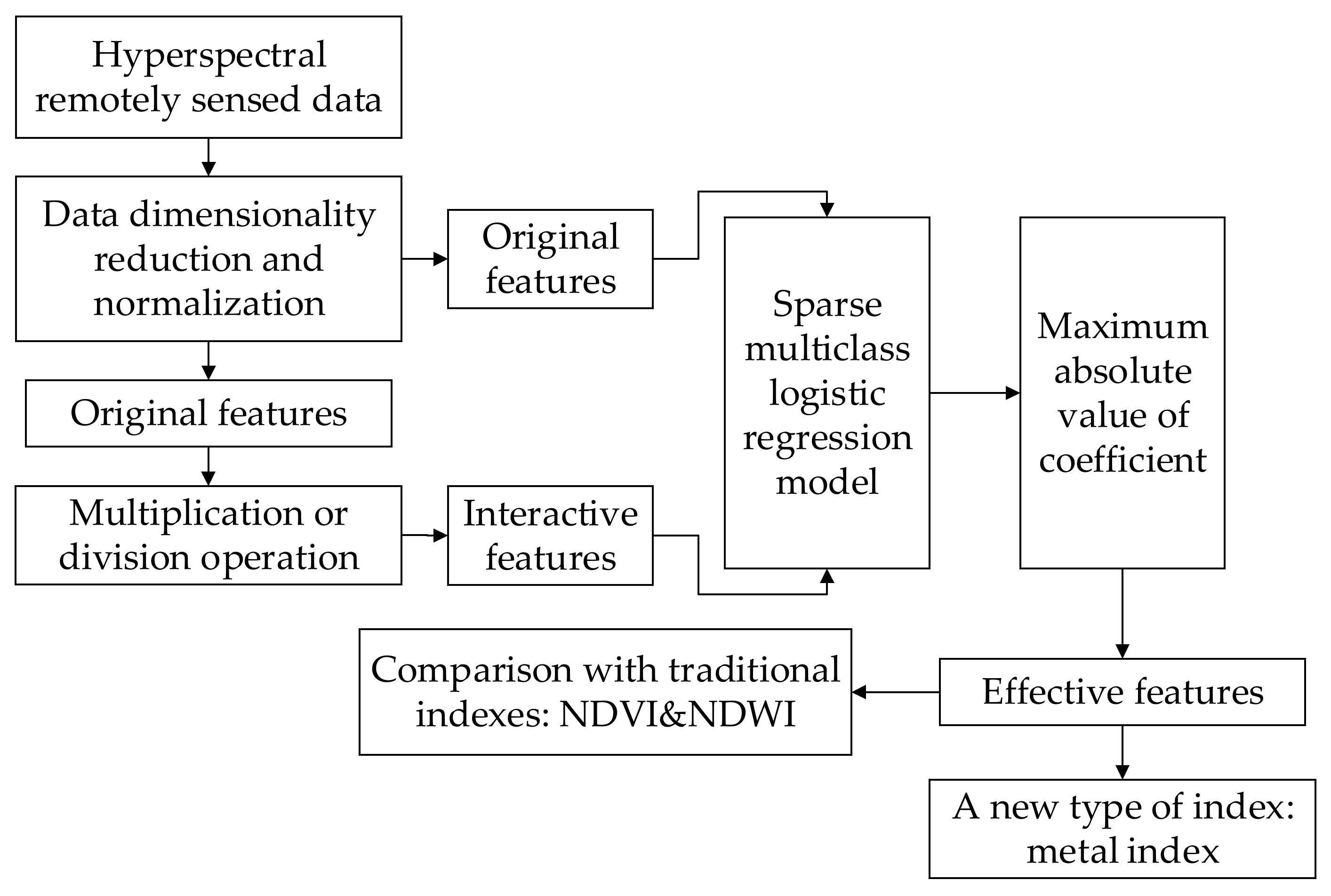
The key point of the method in this paper is explicitly to express the interaction relationship between original features as new features by multiplication or division operation in the logistic regression. This method automatically learns effective features based on data dimensionality reduction and normalization of hyperspectral remotely sensed images. Then the method uses these effective features as new indexes to extract ground features, subsequently compare them with the traditional indexes obtained by laboratory research. Meanwhile, a new type of metal index is proposed. Finally, the method of visual interpretation is used to evaluate the results, together with two indicators: OA (Overall Accuracy) and Recall. The overall technique flowchart is shown in Figure 1.

2.1. Hyperspectral Image Preprocessing

Hyperspectral remote sensing imagery has the characteristics of extremely high spectral resolution. At the same time, it also brings about the problem of high data dimension and a large amount of redundant information between adjacent bands [27]. Therefore, in order to avoid redundant information, data dimensionality reduction is required [28]. Considering that adjacent bands have similar spectral characteristics, the median value is calculated every 9 bands and used as the representative band, which greatly reduces the amount of experimental data. The pixel values of all bands of the image are normalized so that all pixel values are limited between 0–1. This is to eliminate the adverse effects of singular sample data and reduce training time. The normalized conversion function is as follows:

$$X=\frac{x-\min (x)}{\max (x)-\min (x)}$$

(1)

Among them, x represents the pixel value in the original image, and X represents the pixel value in the normalized image.

2.2. Representation of Interaction between Features

For the problem of remote sensing feature extraction, considering the interaction between spectral features will enhance the independence between categories and improve the recognition accuracy of different categories. The most typical example is the NDVI, which uses the ratio of reflectivity between the R (red) band and the NIR (near-infrared) band to improve vegetation identification. Similarly, NDWI, NDBI, etc. all use the interaction between bands. These ratio indexes come from the analysis of the spectral characteristics presented in laboratory observations and remotely sensed data. The purpose of this article is to express the interaction relationship between original features as new features by multiplication or division operation and generalize these ratio indexes.

For a logistic regression with K-category, the softmax transformation can be used as the discriminative model to calculate the posterior probability directly for the response variable belonging to class k:

$$P({\mathrm{Y}}^{(k)}=k|\mathrm{X},\alpha )=\frac{\exp ({\displaystyle \sum _j{\alpha }_j{}^{(k)}{X}_j})}{{\displaystyle \sum _{i=1}^K\exp ({\displaystyle \sum _j{\alpha }_j{}^{(i)}{X}_j})}}$$

(2)

Among them, ${\rm X}=\left\{X_1,X_2,\dots ,X_P\right\}\subset {ℝ}^P$ is a P-dimensional predictor variable and $\mathrm{Y}\subset {ℝ}^K$ represents the response variable, $K$ is the total number of classes, $\alpha$ is the vector of parameters for each classes regression, ${\alpha }_j{}^{\left(k\right)}$ is the jth parameter for class k.

The interaction between features is often expressed as a paired product relationship:

$$P({\mathrm{Y}}^{(k)}=k|\mathrm{X},\alpha )=\frac{\exp ({\displaystyle \sum _j{\alpha }_j{}^{(k)}{X}_j}+{\displaystyle \sum _{j,k}{\alpha }_{jk}{X}_j{X}_k})}{{\displaystyle \sum _{i=1}^K\exp ({\displaystyle \sum _j{\alpha }_j{}^{(i)}{X}_j}+{\displaystyle \sum _{j,k}{\alpha }_{jk}{X}_j{X}_k})}}$$

(3)

the summation part ${\displaystyle \sum _j{\alpha }_j{}^{(k)}{X}_j}$ represents the main feature item, and the quadratic term ${\displaystyle \sum _{j,k}{\alpha }_{jk}{X}_j{X}_k}$ represents the item of the interaction relationship between the features.

Based on the interaction framework of Equation (3), the interaction between features can be expressed in the form of a ratio, which can be further written as:

$$P({\mathrm{Y}}^{(k)}=k|\mathrm{X},\alpha )=\frac{\exp ({\displaystyle \sum _j{\alpha }_j{}^{(k)}{X}_j}+{\displaystyle \sum _{j,k}{\alpha }_{jk}{}^{(k)}\frac{X_j}{X_k}})}{{\displaystyle \sum _{i=1}^K\exp ({\displaystyle \sum _j{\alpha }_j{}^{(i)}{X}_j}+{\displaystyle \sum _{j,k}{\alpha }_{jk}{}^{(i)}\frac{X_j}{X_k}})}}$$

(4)

The purpose of changing the form of the product is to capture the phenomenon similar to NDVI or NDWI. The advantage of this formula is that it covers all the pair-wise ratio relationships between features. However, not all the ratio relationships of the feature pairs contribute to the separation of feature categories, so it is necessary to find the ratio of useful feature pairs, sparse optimization is an effective method.

2.3. Autonomous Learning Based on Sparse Multiclass Logistic Regression

The core of sparse optimization is to use the L1 norm as the constraint term of the regression problem. Although both the L1 norm and the L2 norm can solve the problem of regression model overfitting, the biggest difference between the two is that the L1 norm can make the part unimportant weight value of the feature becomes 0, so as to achieve the effect of sparse model coefficients. The estimated value of the sparse model with the L1 norm is expressed as follows:

$$\widehat{\alpha }=\arg \min \left\{{\displaystyle \sum _{i=1}^n\left[{\left(y_i-{\displaystyle \sum _j{\alpha }_j{x}_{ij}}\right)}^2+\lambda {\displaystyle \sum _j\left|{\alpha }_j\right|}\right]}\right\}$$

(5)

Among them, n is the number of samples, $x_{ij}$ represents the predictor variable, $y_i$ is the dependent variable of the predictor variable. The smaller the penalty coefficient $\lambda$, the lower the degree of compression, and the more variables that are not 0; on the contrary, the larger $\lambda$, the greater the degree of compression, and the fewer variables that are not 0.

With the development of the Least Absolute Shrinkage and Selection Operator (LASSO), logistic regression has more fields for applications. Meier extended the Lasso group (gLasso) to logistic regression for high-dimensional problems and generalized linear model to solve the corresponding convex optimization problem [29]. After Böhning proposed multiclass logistic regression [30], Lasso’s contraction estimation method can be extended to multiclass logistic regression, and the resulting likelihood function of multiclass logistic regression can be written as:

$$L(y|\alpha )={\displaystyle \prod _{i=1}^n{{\displaystyle \prod _{k=1}^K\left(\frac{\exp ({\alpha }^{(k)}{x}_i)}{{\displaystyle \sum _{l=1}^K\exp ({\alpha }^{(l)}{x}_i)}}\right)}}^{y_i{}^{\left(k\right)}}}$$

(6)

where $x_i$ is the P-dimensional feature vector and $y_i$ is the vector of the K-dimensional category label. When the cross-entropy error function is used for multiclass problems, the goal of maximum likelihood estimation can be achieved by minimizing the negative log-likelihood function:

$$E(\alpha )=-\ln L\left(y|\alpha \right)$$

$$=-{\displaystyle \sum _{i=1}^n\left({\displaystyle \sum _{k=1}^K{y}_i{}^{\left(k\right)}{\alpha }^{\left(k\right)}{x}_i+\ln \left({\displaystyle \sum _{l=1}^K\exp \left({\alpha }^{\left(l\right)}{x}_i\right)}\right)}\right)}$$

(7)

The sparse representation can eliminate unimportant features from high-dimensional data and leave effective features [31]. Therefore, this paper introduces the L1 norm on the basis of the multiclass logistic regression model, and the parameter estimation is in the following form:

$$\alpha =\arg \min \left\{E\left(\alpha \right)+\lambda {\displaystyle \sum _j^P\underset{k=1,2\dots K}{\max }\left(‖{\alpha }^{\left(k\right)}‖\right)}\right\}$$

(8)

$‖{\alpha }^{\left(k\right)}‖$ represents the L1 norm as a penalty term of the likelihood function. In this way, the sparse processing of the parameters is performed, and many components that are not important to the category are set to zero. However, this process completes high-dimensional data classification and feature selection, and the parameters will be estimated by cross-validation in the experiment. The proposed method is described as follows (Algorithm 1).

Algorithm 1 The modified SMLR model for autonomous learning

Input: An HSI dataset $X$ and the corresponding label vectors $Y$, the shape of $X$ is

$\left(H\times W\right)\times C$ and the shape of $Y$ is $\left(H\times W\right)\times 1$

Step1: Normalize the pixel values of all bands of the image between 0 and 1.

Step2: Calculate the median value for every 9 bands, the shape of the dataset is changed to

$\left(H\times W\right)\times C_1$, $C_1=⌊C/9⌋+1$. Then, calculate the interaction between any two bands and

express it as $\frac{X_j}{X_k}$, which can be seen in equation (4).

Step3: Randomly divide the HSI dataset $X$ into $X_1$ and $X_2$, which represent the training data and testing data. Likewise, $Y_1$ and $Y_2$ are the corresponding label vector.

Step4: Input $X_1$, $X_2$ and $Y_1$, $Y_2$ into modified SMLR model for autonomous learning.

Step5: Get the optimal penalty coefficient $\lambda$ through 5-fold cross-validation on the sample data

Step6: According to (6)–(8), calculate the coefficient of class k corresponding to each band, and through automatic learning, some unimportant band coefficients become 0.

Step7: The feature expression corresponding to the largest coefficient is used as the index of the extraction class k.

Output: Feature extraction results

3. Experimental Data

3.1. Pavia University Data Set

The data of Pavia University is obtained by ROSIS sensors. There are 115 bands in total, ranging from 0.43 to 0.86 μm. After processing, there are 103 bands. The data image size is 610 pixels × 340 pixels and its spatial resolution is 1.3 m. The spectral resolution is 3.74 nm. It contains 9 feature types, namely: asphalt, meadows, gravel, trees, metal, bare soil, bitumen, bricks, and shadows. Figure 2 shows the false-color composite image and ground truth information of the data set, and

Table 1. Land category and sample size of Pavia University data set.

#	1	2	3	4	5	6	7	8	9
Category	Asphalt	Meadows	Gravel	Trees	Metal	Bare soil	Bitumen	Bricks	Shadows
Size	6631	18649	2099	3064	1345	5029	1330	3682	947

shows the corresponding categories and sample size.

3.2. Pavia Center Data Set

The data of the Pavia Center was acquired by ROSIS sensors over Pavia in northern Italy. There are 115 bands, ranging from 0.43 to 0.86 μm, and there are 102 bands after processing. The size of the data image is 1096 pixels × 715 pixels, and the spatial resolution of each pixel is 1.3 m. The spectral resolution is 3.74 nm. It contains 9 feature categories, namely: water, trees, meadow, block, bare soil, asphalt, bitumen, bricks, and shadows. Figure 3 is a false-color composite image of the data set and ground truth information.

Table 2. Land category and sample size of Pavia Center data set.

#	1	2	3	4	5	6	7	8	9
Category	Water	Trees	Meadow	Block	Bare soil	Asphalt	Bitumen	Bricks	Shadows
Size	65972	7599	3091	2686	6585	9249	7288	42827	2864

shows the type and size of samples of the data set.

3.3. Washington DC Mall Dataset

The data is acquired by the Hydice sensor and collected by the Virginia Spectrum Information Technology Application Center. The data includes a total of 210 bands ranging from 0.4 to 2.4 µm, omitting the atmospheric opaque areas in the 0.9 and 1.4 µm regions. There are 191 bands left, and the data size is 1280 pixels × 307 pixels. The spectral resolution is 10 nm. Feature categories include roof, block, gravel, meadow, trees, water, and shadows. Figure 4 shows the false-color composite map and ground truth information of the data set, and

Table 3. Land category and sample size of Washington DC Mall data set.

#	1	2	3	4	5	6	7
Category	Roof	Block	Gravel	Meadow	Trees	Water	Shadows
Size	3834	416	175	1928	405	1224	97

shows the types of ground features and the number of samples.

4. Experimental Results and Analysis

Normalized Difference Vegetation Index (NDVI), Normalized Difference Water Index (NDWI), Normalized Difference Building Index (NDBI), etc. are all manifestations of the interaction between bands in a ratio [32]. Among them, NDVI is expressed as (NIR − R)/(NIR + R), which is related to the reflection value of the NIR band and the R band. The above indexes are obtained through a large number of experiments in the laboratory. This article aims to use a data-driven method to learn interactive features for hyperspectral remotely sensed data based on a sparse multiclass logistic regression model. These features used as new indexes are compared with the indexes obtained by the traditional method. This experiment only takes vegetation and water body as objects for analysis, and subsequent research can be further extended to more types of ground features.

The interaction relationship between original features is expressed as new features by multiplication or division operation, which can be used as a new index for extracting ground feature information. When considering the interaction between bands in the experiment, the following methods are used to reduce data redundancy and make the amount of calculation controllable: considering that in hyperspectral data, adjacent bands have similar spectral characteristics, it is calculated once every 9 bands The median value is used as a representative. It should be noted that only the median value in the odd number of bands can retain the information characteristics of the original band. If the average value or the median value in the even number of bands is taken, the original band needs to be averaged, which will destroy the characteristics of the original band. The reason why we chose 9 bands has been illustrated in Section 4.4. In addition, continuous strengthening of L1 regularization will make the feature matrix sparse. When automatically learning the interaction relationship, if the feature dimension is greater than the number of training samples, the sparsity of the L1 norm is required to reduce the feature dimension, so the use of the interaction between bands to determine the type of features needs to rely on the sparsity of the L1 norm.

4.1. Extraction of Vegetation and Water Body in the Pavia Center Data Set

For the Pavia Center data set with the interaction between bands, 0.5% of each type of feature is selected as the training sample. If the regularization coefficient is too large, it will easily cause under-fitting, and if it is too small, it will easily cause over-fitting. Therefore, the most suitable regularization coefficient is selected automatically through 5-fold cross-validation and controls the value of the regularization coefficient within the range of 0.01 to 100, and the number is set to 30. When the cross-validation error is the smallest, the value of the optimal regularization parameter is 16.7, Since the water body information in the data set is relatively rich, the feature selection for the water body type is shown in

Table 4. Feature selection of water body.

Category	Features
Water	88, 94, 101, BAND13, BAND32, BAND55

:

88, 94, 101 represent the original band88, 94, and 101, and the corresponding wavelengths are 865 nm, 895 nm, and 930 nm, which belong to the NIR band; BAND13, BAND32, and BAND55 indicate the bands that are added to the interaction by multiplication or division operation. The naming rules for the interaction bands are: for example, the original bands remaining after dimensionality reduction are a band a, band b, band c, band d, and band e, then BAND1 is expressed as the interaction between band a and band b, BAND2 It is expressed as the interaction between band a and band c until BAND4 is expressed as the interaction between band a and band e, the interaction between band a and other bands except itself indicates the end, and then BAND5 indicates the interaction between band b and band c until the interaction of band b and other bands except itself indicates the end, and so on until BAND10 indicates the interaction of band d and band e, so far all the interaction indicates completion. BAND13 means (band11-band44)/(band11 + band44). The wavelength of band11 is 480 nm and belongs to the B (blue) band. The wavelength of band44 is 645 nm and belongs to the R band. So BAND13 describes the interaction between B and R bands. In the same way, BAND32 means (band34-band88)/(band34 + band88) and describes the relationship between G (green) and NIR bands; BAND55 means (band94-band101)/(band94 + band101) and describes the interaction between the NIR bands. The specific interaction relationship is shown in

Table 5. Interaction characteristic coefficients of water body.

Features	88	94	101	BAND13	BAND32	BAND55
Coefficient	−2.189	−2.941	−1.082	−0.751	5.706	1.574

:

From the coefficients of multiclass logistic regression, BAND32 has the most prominent regression coefficient among all the characteristics, indicating that BAND32 is the most sensitive to water body information and has the best effect on water body recognition. Therefore, BAND32 is used as an interactive water index, which is expressed as follows:

$$\mathrm{B}\mathrm{A}\mathrm{N}\mathrm{D}32=\frac{\mathrm{band}34-\mathrm{band}88}{\mathrm{band}34+\mathrm{band}88}=\frac{G-NIR}{G+NIR}$$

(9)

The same method for the feature selection of the feature type of tree is shown in

Table 6. Interactive feature coefficients of vegetation.

Features	BAND47	BAND48	BAND49
Coefficient	0.769	0.800	0.094

:

BAND47 represents the interaction between band66 and band88, the wavelength of band66 is 755 nm, which means the R band, and the wavelength of band88 is 865 nm, which represents the NIR band. In the same way, BAND48 and BAND49 are also expressed as the interactive relationship between the R band and the NIR band. Since the regression coefficients of BAND47 and BAND48 are larger than BAND49, it means that for vegetation information, BAND47 and BAND48 have a better recognition effect. Analogous to the expression form of the normalized index, BAND48 can be expressed as:

$$\mathrm{B}\mathrm{A}\mathrm{N}\mathrm{D}48=\frac{\mathrm{band}66-\mathrm{band}94}{\mathrm{band}66+\mathrm{band}94}=\frac{R-NIR}{R+NIR}$$

(10)

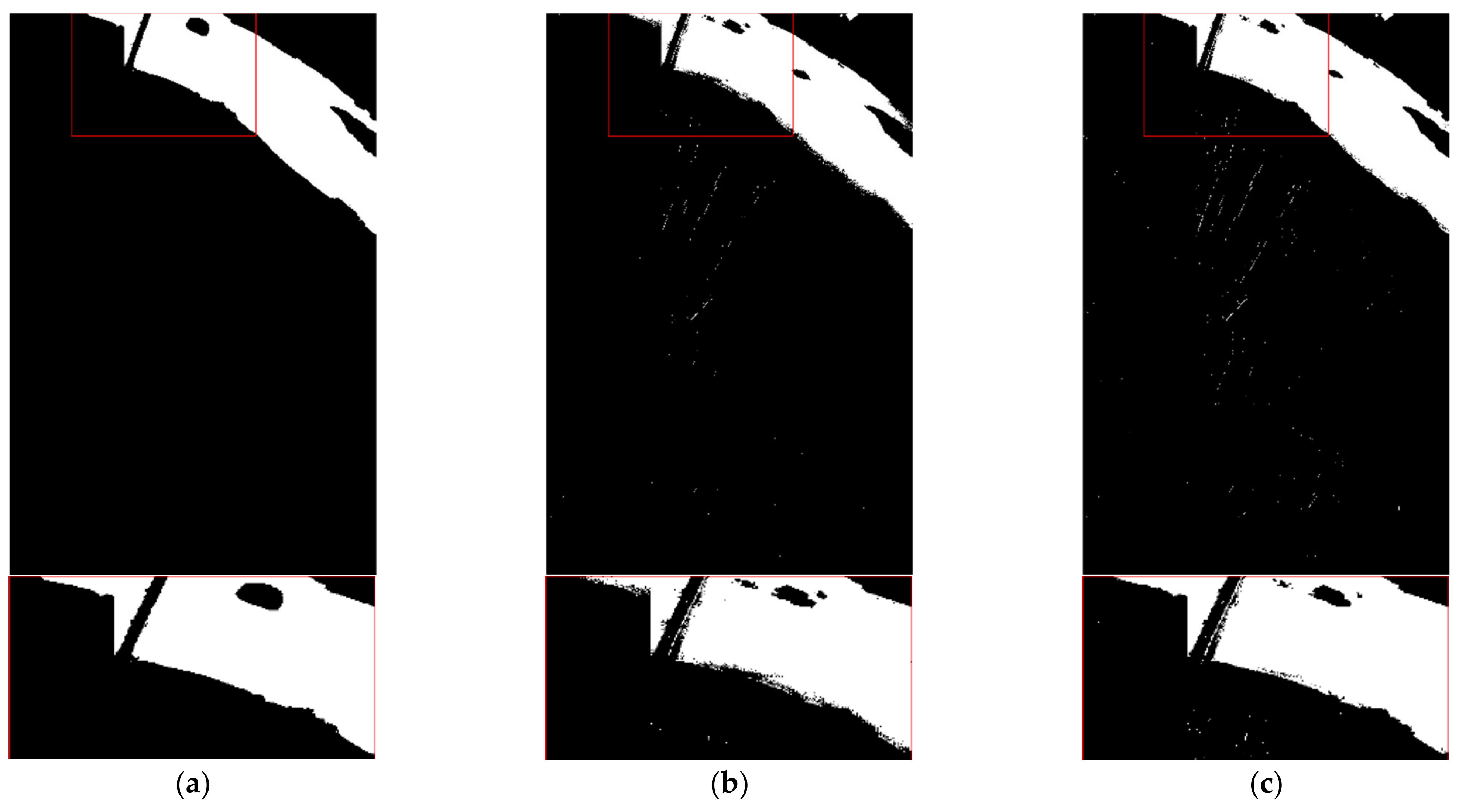
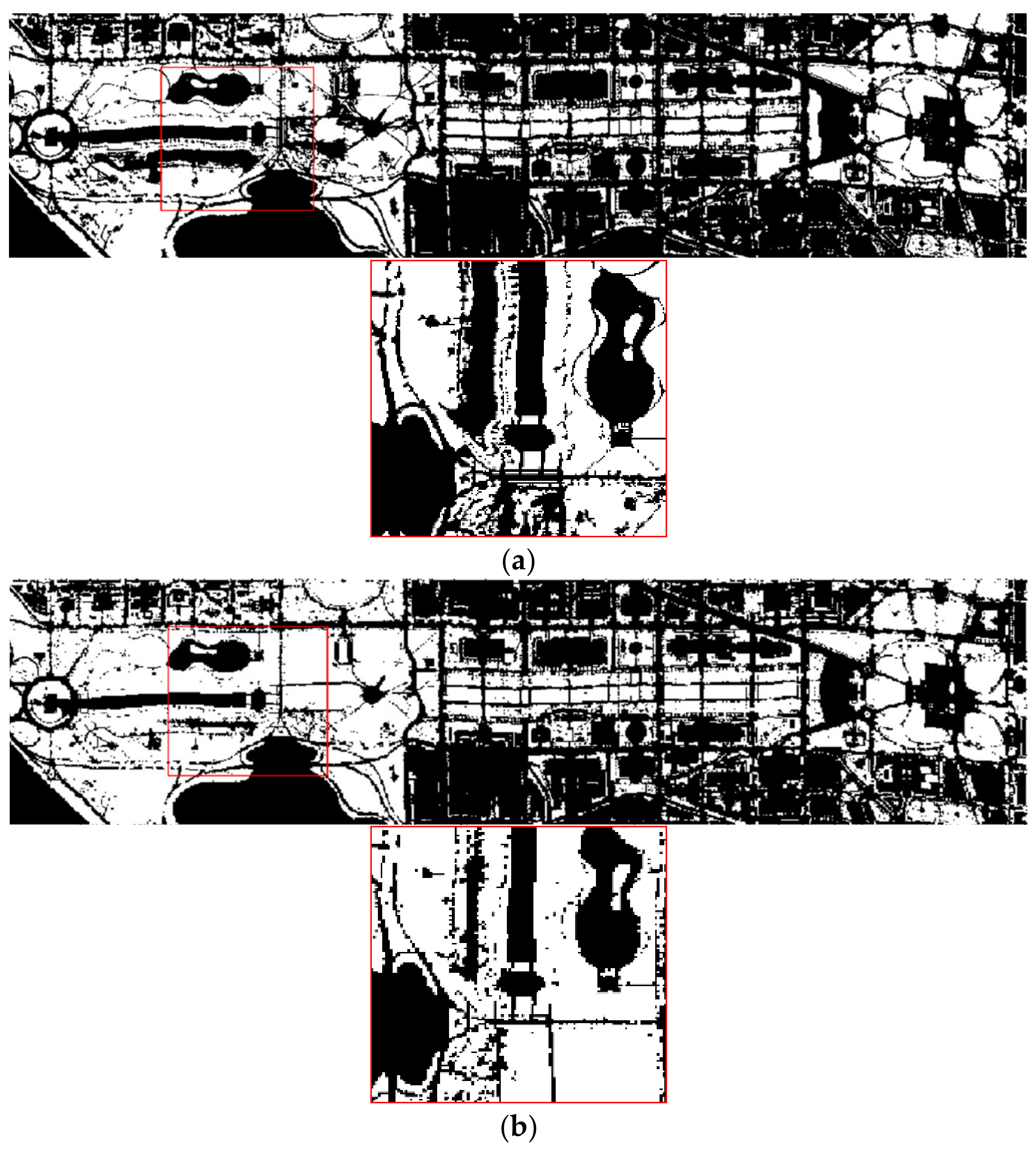
Compared with NDVI, it can be proved that the interactive relationship between BAND47 and BAND48 can be used as an interactive vegetation index. In order to display the results more intuitively, BAND32 and BAND48 are used as the water body index and vegetation index to extract the water body and vegetation in the Pavia Center data set, and the results of the water body extracted by BAND32 are compared with the results of NDWI, which was extracted by the laboratory. Results of vegetation extracted by BAND48 are compared with NDVI, as shown in Figure 5 and Figure 6:

BAND32 can effectively extract water body and is similar to the extraction results of NDWI; BAND48 can also effectively extract vegetation and is similar to the extraction results of NDVI. To make the result clearer, the accuracy of the correctly extracted pixels in the binary image is counted. The pixel value 0 represents black (background), and the pixel value 255 represents white (target features). The quantitative results of the water body are shown in

Table 7. Quantitative comparison results of water extraction from the Pavia Center data set.

Category	Recall of NDWI	Recall of BAND32
0	0.998	0.997
255	0.915	0.969
Overall Accuracy	0.989	0.994

. The quantitative results of vegetation are shown in

Table 8. Quantitative comparison results of vegetation extraction from the Pavia Center data set.

Category	Recall of NDVI	Recall of BAND48
0	0.982	0.979
255	0.783	0.833
Overall Accuracy	0.935	0.945

. The accuracy of BAND32 and BAND48 for the correct extraction of water body and vegetation is higher than that of NDWI and NDVI.

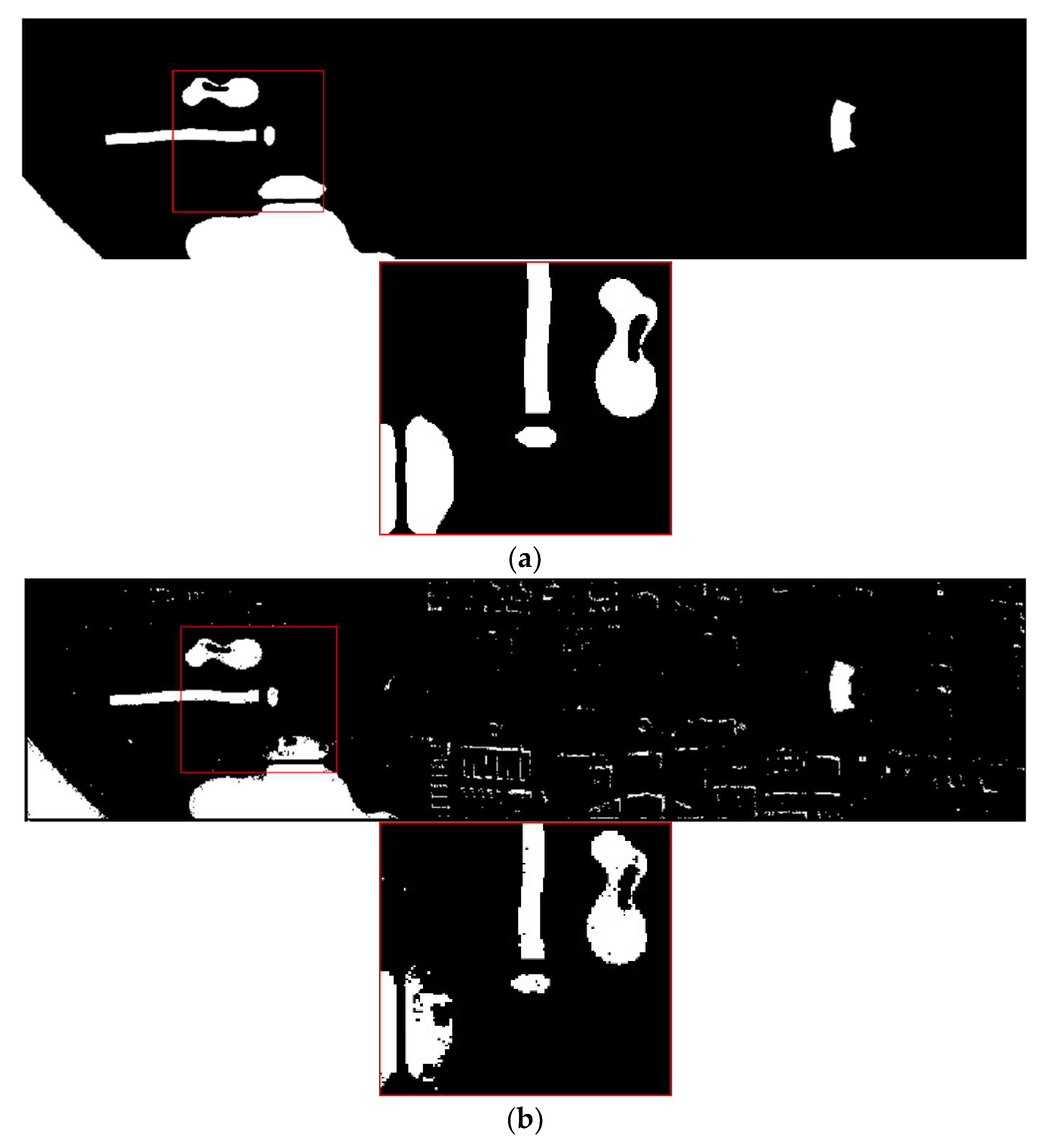
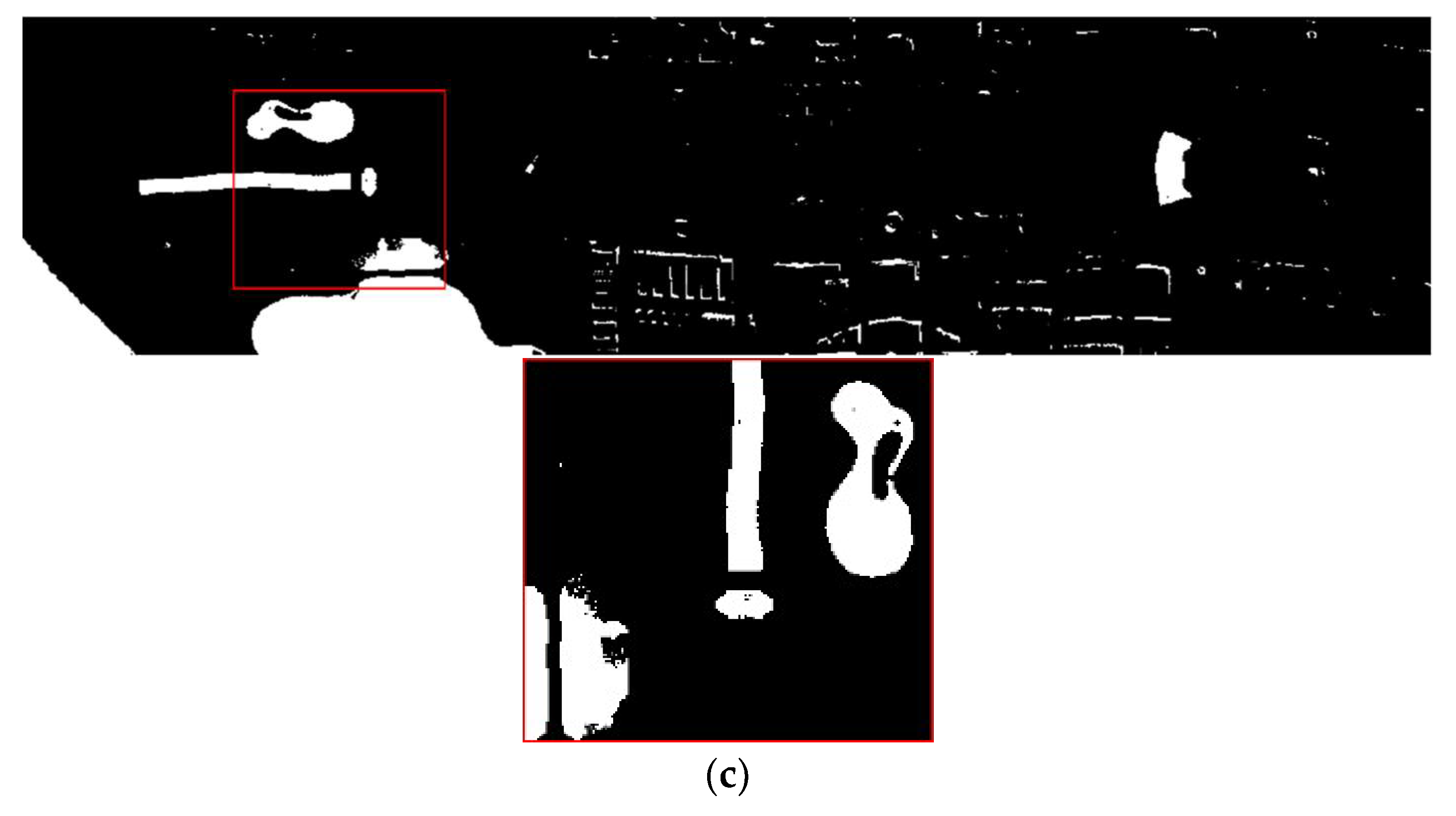
4.2. Extraction of Vegetation and Water Body in the Washington DC Mall Dataset

For the Washington DC Mall data set, because the number of samples is small, 4% of each type of feature is selected as the training sample, and the optimal regularization parameter obtained by 5-fold cross-validation is 25. At this time, the feature matrix is very sparse, with only one feature of water body and vegetation, as shown in

Table 9. Interaction characteristic coefficients of water body and vegetation.

Category	Interactive Features	Coefficient
Water	BAND9	0.022
Meadow	BAND41	−0.09

:

BAND9 and BAND41 can be expressed as:

$$\mathrm{BAND}9=\frac{\mathrm{band}6-\mathrm{band}95}{\mathrm{band}6+\mathrm{band}95}=\frac{purple-NIR}{purple+NIR}$$

(11)

$$\mathrm{BAND}41=\frac{\mathrm{band}26-\mathrm{band}85}{\mathrm{band}26+\mathrm{band}85}=\frac{G-NIR}{G+NIR}$$

(12)

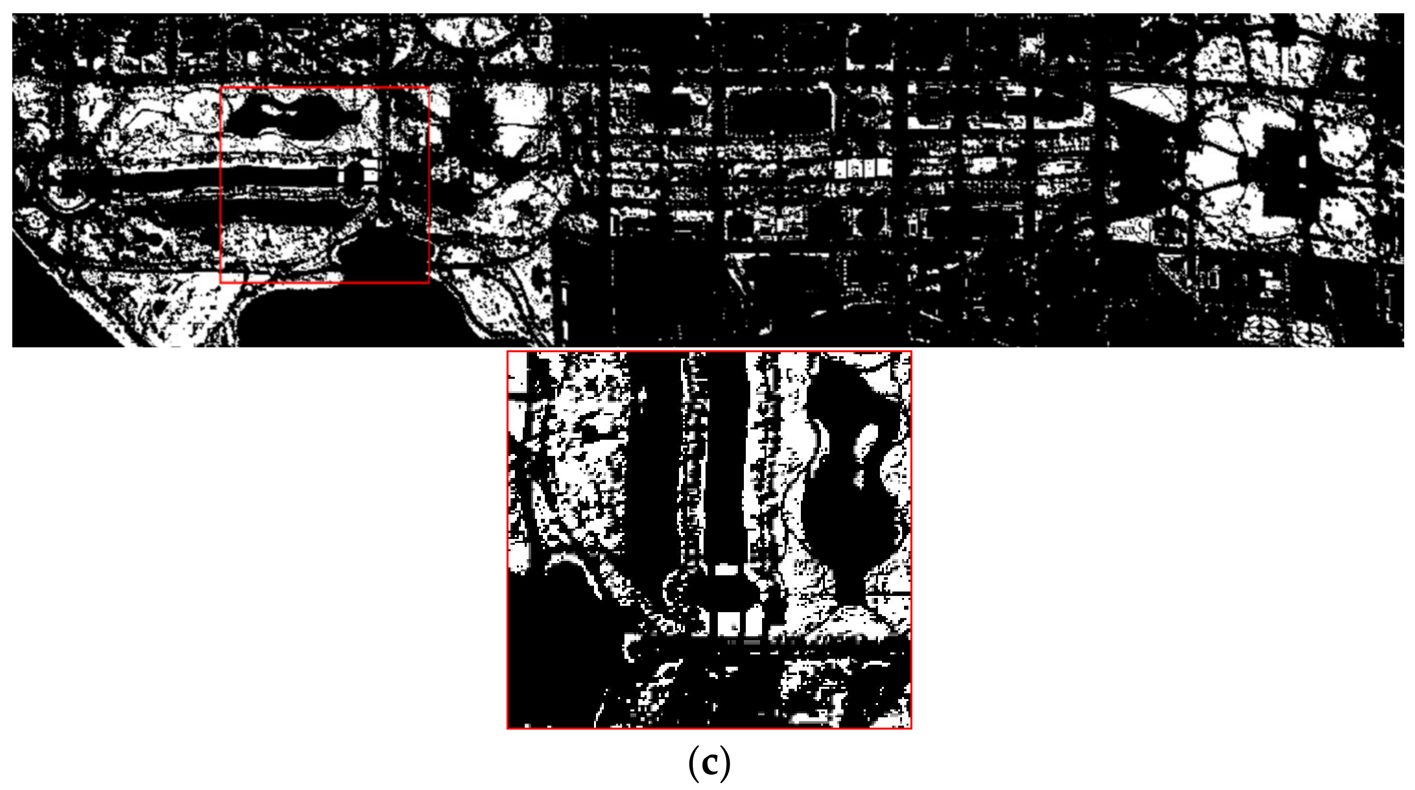
The wavelength of band6 is 418 nm, which corresponds to the purple light band, so it is named “purple”; the wavelength of band95 is 1248 nm, which corresponds to the NIR band. The wavelength of band26 is 498 nm corresponding to the G band, and the wavelength of band85 is 1099 nm corresponding to the NIR band. The above two expressions seem to be inconsistent with those of NDVI and NDWI. To verify the experimental results, BAND9 and BAND41 were used to extract water body and vegetation respectively. Then BAND9 is compared with NDWI in terms of water extraction; BAND41 is compared with NDVI in terms of vegetation extraction, as shown in Figure 7 and Figure 8:

From visual judgment, both the effect of BAND9 in extracting water body and the effect of BAND41 in extracting vegetation are similar to those of NDWI and NDVI. To display the extraction results more clearly, the extraction results of water and vegetation are also quantified. The quantitative results of water body are shown in

Table 10. Quantitative comparison results of water extraction from the Washington DC Mall data set.

Category	Recall of NDWI	Recall of BAND9
0	0.942	0.939
255	0.209	0.251
Overall Accuracy	0.893	0.893

; the quantitative results of vegetation are shown in

Table 11. Quantitative comparison results of vegetation extraction from the Washington DC Mall data set.

Category	Recall of NDVI	Recall of BAND41
0	0.613	0.862
255	0.458	0.223
Overall Accuracy	0.551	0.605

.

It can be seen from Table 10 that for the extraction of water body, the extraction overall accuracy of BAND9 and NDWI are almost the same as 0.893, but for the water body category (pixel value 255), BAND9′s 0.251 is better than NDWI’s 0.209; from Table 11 we can see that for vegetation, the number of pixels correctly extracted by BAND41 is less than NDVI, but the overall accuracy of BAND41 is better than NDVI.

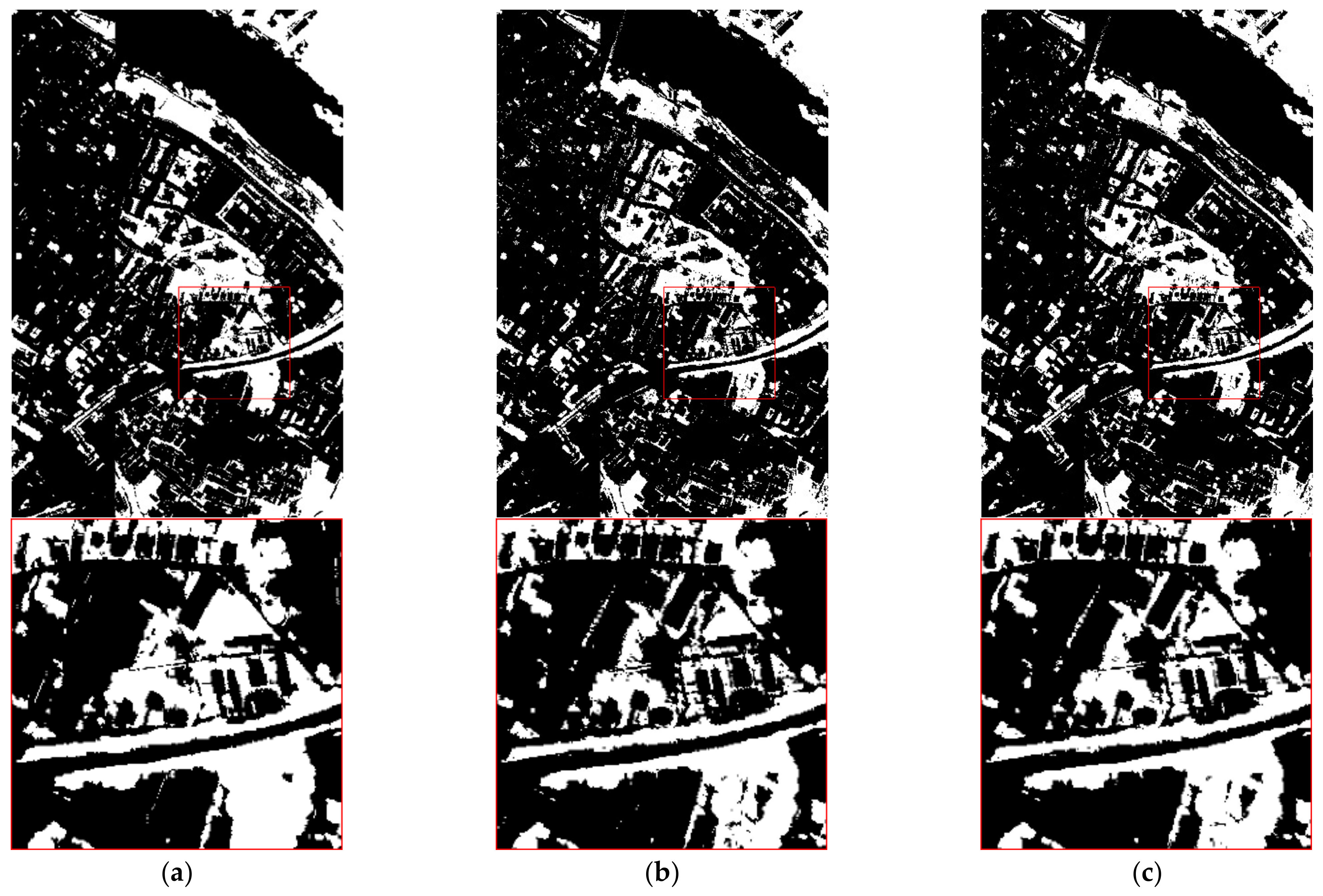
4.3. Extraction of Vegetation from the Data Set of the University of Pavia

For the Pavia University data set, 0.5% of each type of ground feature is selected as the training sample. Because the vegetation information in the data set is relatively rich and there is no water body information, only the vegetation part is tested. The 5-fold cross-validation shows that the value of the regularization parameter is 10. At this time, the feature matrix becomes very sparse, and the interactive features of the vegetation part can be seen in

Table 12. Interaction characteristic coefficients of vegetation.

Feature	BAND18	BAND19
Coefficient	0.73	0.87

.

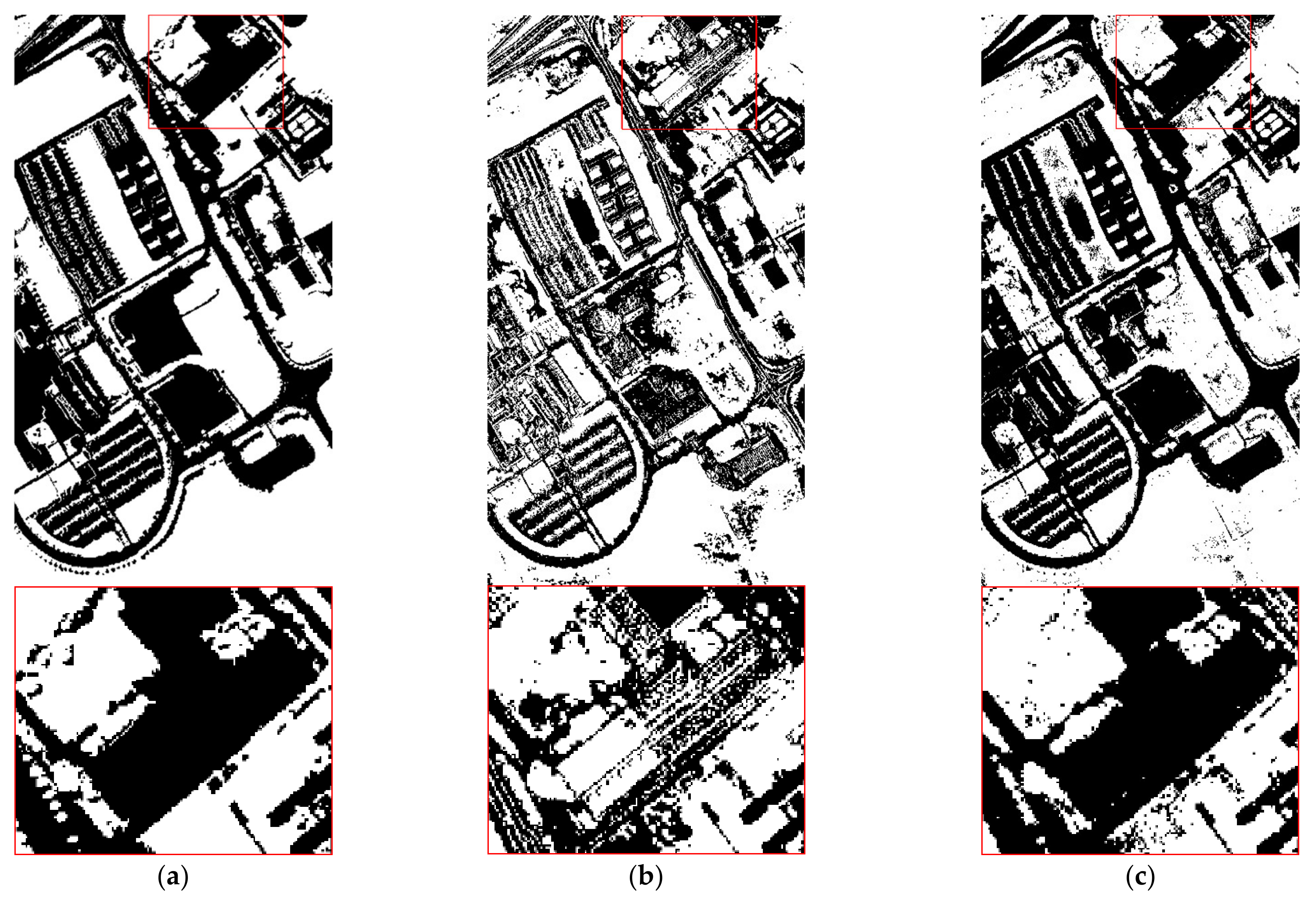
Compared with BAND18, BAND19 is more prominent. The coefficient of BAND19 is larger, indicating that the feature is more important, which can be expressed as:

$$\mathrm{BAND}19=\frac{\mathrm{band}11-\mathrm{band}94}{\mathrm{band}11+\mathrm{band}94}=\frac{B-NIR}{B+NIR}$$

(13)

Among them, the wavelength of band11 is 480 nm belonging to the B band, and the wavelength of band94 is 895 nm, which belongs to the NIR band. The vegetation is extracted by BAND19, and the binarization results are shown in Figure 9:

BAND19 is significantly better than NDVI in the Pavia University data set for vegetation extraction. To make the results more convincing, quantitative results are also given, as shown in

Table 13. Quantitative comparison results of vegetation extraction from the Pavia university data set.

Category	Recall of NDVI	Recall of BAND19
0	0.677	0.909
255	0.844	0.882
Overall Accuracy	0.768	0.895

.

For the extraction of vegetation, BAND19 is significantly better than NDVI, which proves the effectiveness of BAND19.

4.4. Supplementary Experiment

This part is used to prove the influence of the number of bands selected when taking the median value on the experimental results. Because the selection of the number of bands is not the main content of this article, in order to make the overall structure of the article clearer, only the quantitative results are shown here. We conducted separate experiments on the cases where the number of bands was 3, 5, 7, 9 and 11, and used the overall accuracy as the verification index, concluding that when the number of bands was 9, the overall extraction result was the best. Although the extraction results of other cases are not as good as the case where the number of bands is 9, they are almost all better than the extraction results of the traditional index. The results are shown in

Table 14. The overall accuracy of vegetation extraction for the different number of bands.

Number	Pavia Center		Washington DC		Pavia University
	NDVI	Ours	NDVI	Ours	NDVI	Ours
3	0.935	0.939	0.551	0.582	0.768	0.791
5		0.951		0.59		0.803
7		0.942		0.611		0.882
9		0.945		0.605		0.895
11		0.942		0.596		0.837

and

Table 15. The overall accuracy of water body extraction for the different number of bands.

Number	Pavia Center		Washington DC
	NDWI	Ours	NDWI	Ours
3	0.989	0.979	0.893	0.892
5		0.981		0.893
7		0.989		0.893
9		0.994		0.893
11		0.981		0.889

.

4.5. The New Feature Index in the Data Set of the University of Pavia

In addition to comparing new features learned by the data-driven method with traditional indexes NDVI and NDWI, a new type of ground feature index can also be learned automatically. In the Pavia University data set, there is a category of features called metal. There is no traditional index that can extract this type of feature. Using the method proposed in this article, we can automatically learn the interactive features of metal. When the regularization coefficient is 1, the coefficient results are shown in

Table 16. Interaction characteristic coefficients of metal plates.

Feature	22	BAND22	BAND23	BAND29
Coefficient	4.51	1.82	0.84	1.06

.

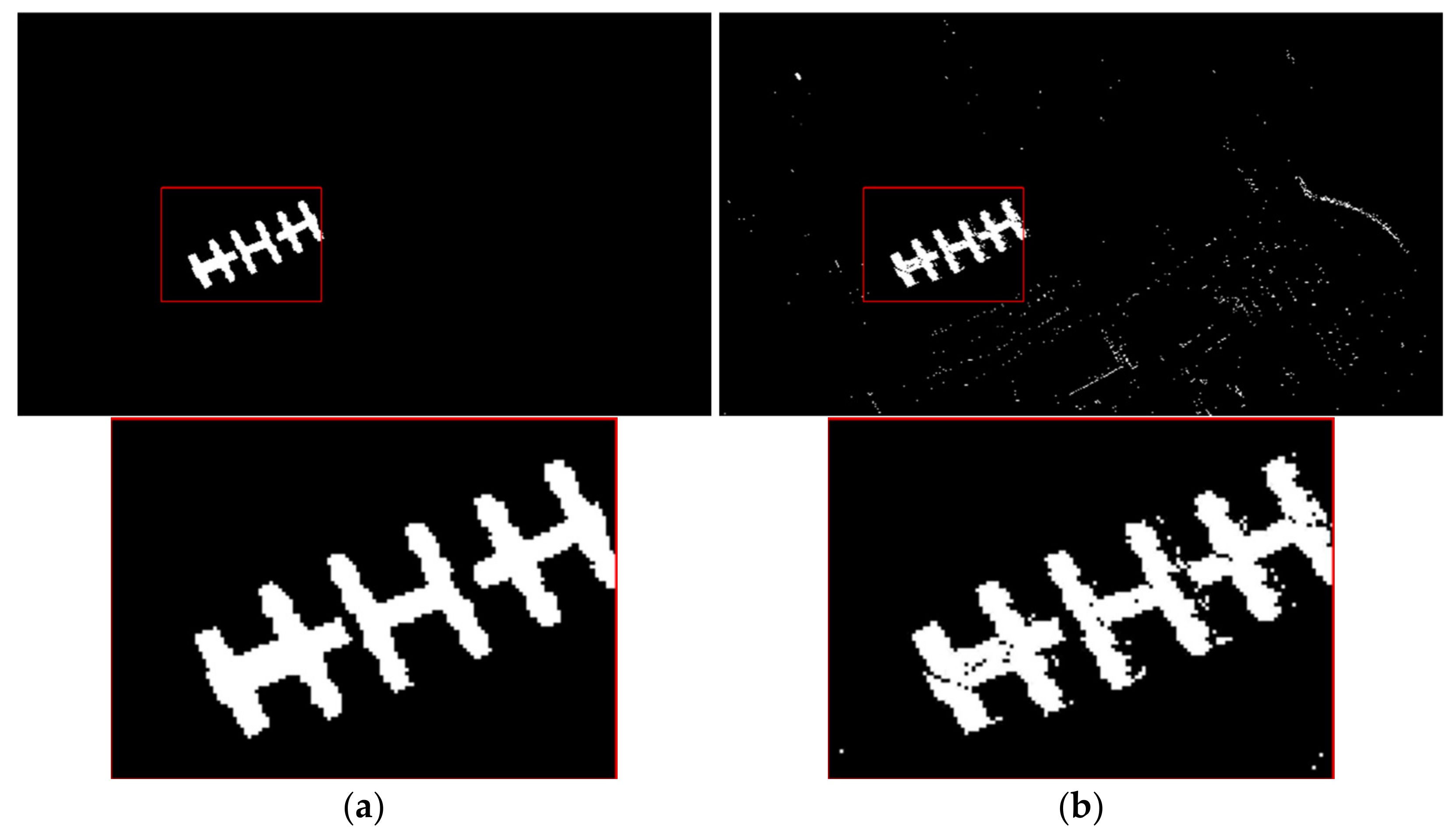
The wavelength of band22 is 535 nm, which represents the G band, indicating that the metals in the data set are more sensitive to the G band. Among interactive features like BAND22, BAND23, and BAND29, BAND22 performs best, and BAND22 can be expressed as:

$$\mathrm{BAND}22=\frac{\mathrm{band}22-\mathrm{band}52}{\mathrm{band}22+\mathrm{band}52}=\frac{G-R}{G+R}$$

(14)

The wavelength of band52 is 685 nm, which represents the R band. The metal is extracted by BAND22, and the binarization result is shown in Figure 10:

BAND22 has an outstanding effect on the extraction of metal, and quantitative results are also given in

Table 17. Quantitative comparison results of metal sheets extraction from the Pavia university data set.

Category	BAND22
0	0.995
255	0.848
Overall Accuracy	0.994

.

The interactive feature BAND22 can be used as a new ground feature index for extracting metals.

5. Conclusions

This paper proposes a data-driven method to learn interactive features for hyperspectral remotely sensed data based on a sparse multiclass logistic regression model. The key point is explicitly to express the interaction relationship between original features as new features by multiplication or division operation, and the strong constraint effect of the L1 norm makes feature sparseness. The size of the coefficient value of the corresponding feature after sparse is used as the basis for judging the importance of the feature, then the most important interactive feature is used as the index for extracting ground features. Significantly, small samples are taken on three hyperspectral remotely sensed data sets. These experiments were carried out separately, and the following conclusions were drawn:

(1) The interaction automatically learned through the data-driven method as a ground feature index can effectively extract water and vegetation. The interaction is expressed by multiplication or division operation between original features. It is shown in the Pavia Center data set that the interactive features BAND32 can extract water body information availably, BAND48 can effectively extract vegetation information; in the Washington DC Mall data set, BAND9 can effectively extract water information, which is almost indistinguishable from NDWI. Although BAND41 does not perform very well with NDVI, it can still extract most of the vegetation information; in the Pavia University data set, the effect of vegetation information extraction with BAND19 is better than NDVI. These interactive relationships learned by the data-driven method can be used as a new type of feature index, which is of great significance to the development of feature recognition.

(2) A new type of metal index BAND22 is proposed in the Pavia University data set, and it is verified with ground truth information of this category. The experimental result proves that the index can effectively extract the ground feature of metal.

The ground feature types explored in this study are only water body and vegetation. In the future, more ground feature types will need to be further studied in order to learn more ground feature indexes. If the verification is effective, it will have pivotal significance on ground features recognition and even social production activities.