1. Introduction
Stroke and spinal cord injury (SCI) are the main causes of human lower limb motor dysfunction [
1,
2,
3]. Motion disability not only causes difficulties with physical control, but also serious psychological problems to the patient, which greatly reduce the quality of life of the patient. Rehabilitation training can effectively help patients with lower limb motor dysfunction improve muscle strength, restore walking ability, and reduce complications [
4]. In terms of the rehabilitation process, the training mode of the robot can be divided into passive training and active training. Passive training requires the robot to drive the patient into predetermined trajectory movement, and the robot usually adopts the control method of trajectory tracking. In this article, aiming at the challenge of low tracking accuracy in trajectory tracking control, research on control methods was carried out to improve the performance of trajectory tracking control.
In the early stage of rehabilitation training, the patient’s lower limbs are almost completely paralyzed (bed-ridden) and rely on external assistance to complete the training action. Traditional rehabilitation gait therapy requires multiple therapists to manually drive the patient’s legs, which increases labor costs [
5], or uses auxiliary equipment connected to the hospital bed to achieve rehabilitation training [
6,
7]. In the early stage of treatment, these approaches are effective, but when the patient leaves the bed for overground gait training, they cannot guarantee better results.
With the emergence of lower limb rehabilitation exoskeleton robots including LOKOMAT [
8] in 2005, HAL [
9] in 2008, ReWalk [
10] in 2010, and ExoMotus [
11] in 2018, a large number of clinical applications have shown that lower limb rehabilitation exoskeleton robots can play good auxiliary roles for patients with different degrees of injury [
12,
13]. Trajectory tracking control, which is one of the main control strategies in the control method of lower limb rehabilitation exoskeleton robots, is the basis and key to realizing different training modes.
The lower limb rehabilitation exoskeleton robot is a multiple-degree-of-freedom open-chain mechanism composed of irregular links that have complex nonlinearity and strong coupling characteristics [
12,
13]. These robots are vulnerable to disturbances from the patient and the ground during the control process. Therefore, it is difficult to establish a complete and accurate mathematical model of the robot, which leads to difficulties in robot motion control and poor trajectory tracking accuracy. Traditional control methods including proportional-integral-derivative (PID) control [
14], computed torque method [
15], adaptive control [
16], and robust control [
17] have difficulty in meeting the actual needs of patients using lower limb rehabilitation exoskeleton robots because their trajectory tracking abilities are limited.
The sliding mode control does not depend on a mathematical model of the controlled object and has strong anti-interference ability and good robustness [
18,
19], consequently, sliding mode controls are widely used in robot control systems [
20]. A sliding mode control divides the motion process of the robot system state into two stages. The first stage is from the initial state to the sliding surface, and the second stage gradually converges to an equilibrium point in the sliding surface [
21]. However, after the system state reaches the sliding surface, it is difficult to strictly slide along the sliding surface to the equilibrium point. Instead, the system state moves back and forth across the sliding surface to approach the equilibrium point, which results in buffeting [
22].
Many researchers have designed reaching laws to change the reaching speed and weaken the chattering of sliding mode controls. Islam et al. [
23] and Nair et al. [
24] proposed a sliding mode control based on the constant velocity reaching law for a lower limb rehabilitation exoskeleton robot. Hao et al. [
25] proposed an adaptive neural network sliding mode control based on the exponential reaching law. Long et al. [
26] proposed a terminal sliding mode control based on the exponential reaching law, and Chen et al. [
27] proposed a terminal sliding mode control based on the exponential reaching law. Devika et al. [
28] proposed a sliding mode control based on the power rate exponential reaching law by combining exponential reaching law and power reaching law. Xia et al. [
29] and Kang et al. [
30] proposed a terminal sliding mode control based on the double-power reaching law. The above studies revealed that the double-power reaching law had a better dynamic quality. In the double-power reaching law, the higher-order power term enables the system state to quickly reach the sliding mode surface when it is far from the surface. Additionally, the lower-order power term enables the approaching speed to decrease gradually as the system states approach the sliding mode surface, which can effectively reduce chattering. The double-power reaching law both weakens the chattering and increases the reaching speed of the system state.
In this article, a self-adaptive-coefficient double-power sliding mode control method was proposed to improve the trajectory tracking accuracy and anti-interference ability of the lower limb rehabilitation exoskeleton robot. The method combines the estimated dynamics model of the robot with sliding mode control based on the double-power reaching law to weaken chattering, and obtains an appropriate reaching speed through a designed self-adaptive-coefficient. First, based on the estimated dynamic model, the estimated control torque of the robot was obtained. Second, based on the double-power reaching law, a compensation term was designed and applied to the estimated control torque to reduce the influence of model error and environmental disturbance. Then, according to the Lyapunov function, a self-adaptive-coefficient of the compensation term was designed to achieve the compensation term following the model error, and a self-adaptive adjustment occurred, which improved the robust performance of the robot. Finally, taking the lower limb rehabilitation exoskeleton robot prototype in laboratory conditions as the controlled object, a co-simulation and a wearable experiment demonstrated that the self-adaptive-coefficient double-power sliding mode control method effectively improved the trajectory tracking accuracy and anti-interference ability of the robot.
3. Self-Adaptive-Coefficient Double-Power Sliding Mode Control Algorithm
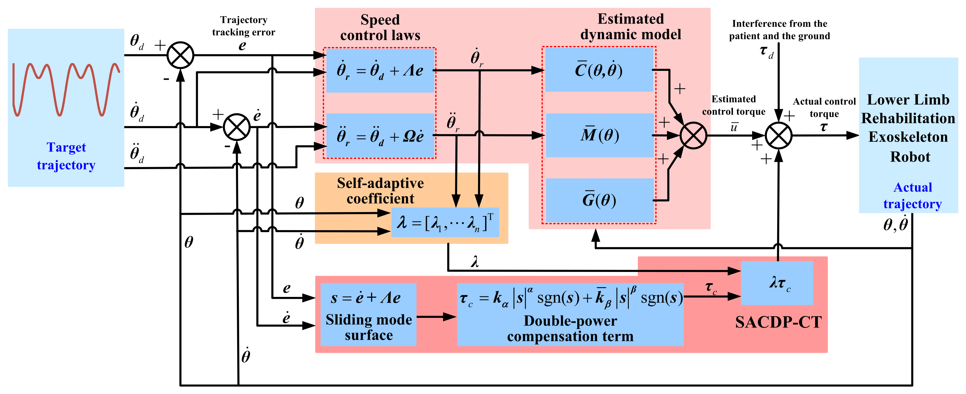
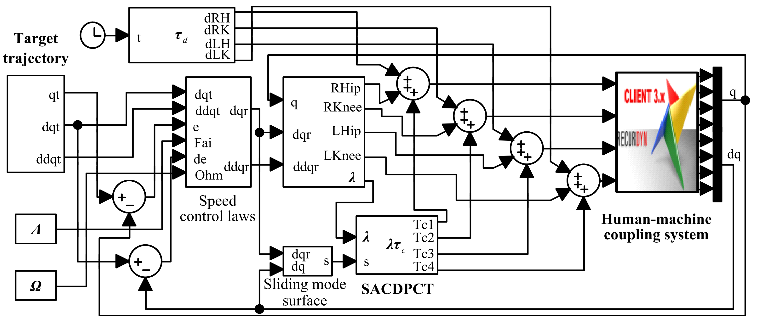
The control block diagram of the self-adaptive-coefficient double-power sliding mode control method is shown in
Figure 3. The design is mainly divided into three parts. Part (I): the dynamic model of the lower limb rehabilitation exoskeleton robot shown in Equation (1) is regarded as an estimated dynamic model. The estimated control torque
is obtained to reduce the nonlinear and strong coupling influences on the robot. Part (II): based on a double-power reaching law, we designed a compensation term
, the sum of the compensation term
, and the estimated control torque
is used as the actual control torque
of the robot to reduce the effects of model error and environmental interference. Part (III): a self-adaptive coefficient
was designed for the compensation term
, and the self-adaptive-coefficient double-power compensation term (SACDPCT)
adjusts adaptively, improving the robust performance of the robot trajectory tracking control.
3.1. Design of Control Law Based on Estimated Model
The patient and the ground environment inevitably interfere with the lower limb rehabilitation exoskeleton robot, which leads to the model error between the established dynamic model and the actual dynamic model. Therefore, this paper regards the established dynamic model as an estimated dynamic model. Using the computed torque method, we designed an estimated control torque based on the estimated dynamic model.
The established dynamic model of the lower limb rehabilitation exoskeleton robot in this paper is shown in Equation (1). Taking the established dynamic model as an estimated dynamic model, we rewrite Equation (1) as follows.
where
is an estimate of the actual inertia matrix
;
is an estimate of the actual centrifugal force and Coriolis force matrix
;
is an estimate of the actual gravity term
; and
is an estimate of the actual control torque
. Therefore, it can be seen from Equation (6):
Considering that the patient and the ground environment will inevitably interfere with the lower limb rehabilitation exoskeleton robot, the actual dynamic model of the lower limb rehabilitation exoskeleton robot can be expressed as follows.
where
is interference, which reflects the interference from the patient and the ground.
, and
is a positive constant matrix.
Because the actual inertial parameters of the lower limb rehabilitation exoskeleton robot cannot be accurately obtained. The actual inertia matrix
, the actual centrifugal force, and Coriolis force matrix
, the actual gravity term
, and the actual interference
are unknown. Based on the computed torque method, a nonlinear feedback control law was designed as the estimated control torque
for each joint of the robot and expressed as follows.
where
and
are the speed control laws to be designed. During the trajectory tracking control of the lower limb rehabilitation exoskeleton robot, the robot needs to track a time-varying target trajectory
. To perform the trajectory tracking of the robot, the speed control laws
and
were designed as follows
where
is the target angular velocity;
is the target angular acceleration;
and
are the positive diagonal matrix;
;
;
is the trajectory tracking error; and
.
According to Equations (6), (8) and (9), based on the computed torque method and the estimated dynamic model, the estimated control torque for each joint of the lower limb rehabilitation exoskeleton robot was designed as follows:
3.2. Design of Compensation Item Based on Double-Power Reaching Law
A sliding mode control allows a robot to maintain system stability under the conditions in which parameters change and environmental interference occurs through the switching of the self-adaptive control [
35]. To reduce the influence of model error and environmental interference on the trajectory tracking of the lower limb rehabilitation exoskeleton robot, its trajectory tracking was achieved by combining the estimated control torque with the sliding mode control method based on a double-power reaching law.
The sliding mode surface
for the sliding mode control was designed as follows:
where the interference
is bounded. Based on the double-power reaching law, the compensation term
for the actual control torque was designed as follows:
where
;
is the symbolic function; and
,
,
,
.
Because and , during the entire sliding phase (), when the system state of the lower limb rehabilitation exoskeleton robot is far from the equilibrium point (e.g., ), the compensation term is determined by the higher-order power term . At this time, makes the high-order power term larger, which effectively increases the approach speed. However, when the system state of the robot is close to the sliding mode surface (e.g., ), the compensation term is determined by the low-order power term . At this point, makes the low-order power term smaller and reduces the reaching speed, which effectively avoids an excessive reaching speed and reduces chattering of the system state.
3.3. Design of Self-Adaptive-Coefficient-Double-Power Sliding Mode Control Method
According to Equations (10) and (12), combining the estimated dynamic model of the lower limb rehabilitation exoskeleton robot and the compensation term based on the double-power reaching law, the control law of the double-power sliding mode control method can be expressed as follows.
We defined the Lyapunov function as follows.
According to Equations (3), (7) and (13), the derivative of Equation (14) with respect to time
is expressed as follows:
where
is the inertial matrix error and
.
is the centrifugal and Coriolis forces error, and
. Here,
is the gravity term error, where
.
Equations (4) and (15) can be expressed as follows.
where
is the linear expression of the model error;
is a known regression matrix about the function of robot joint variables;
;
; and
is a constant parameter vector that describes the quality characteristics of the robot, where
,
,
, and
. Therefore,
From Equation (16),
,
, and
determine whether the control system of the lower limb rehabilitation exoskeleton robot is closed-loop stable. To ensure the stable convergence of the control system, it is necessary to be satisfied as follows.
To enhance the stable convergence of the control system and ensure that the compensation term follows the model error, adjusts adaptively, and improves the anti-interference ability of the robot control system, a self-adaptive-coefficient
was designed for the compensation term
and
as follows.
According to Equations (12) and (19), we rewrite Equation (16) as follows.
From Equation (20), we can see that
. According to LaSalle’s theorem [
36], when
,
. Thus
,
. Therefore, the introduction of the self-adaptive-coefficient
can make
and ensure that the control system of the lower limb rehabilitation exoskeleton robot is closed-loop stable.
In addition, the self-adaptive-coefficient is determined by the model error . Therefore, can follow the model error and self-adaptive adjustment, thereby enhancing the anti-interference ability of the control system.
In summary, the control law of the self-adaptive-coefficient double-power sliding mode control method proposed in this paper is shown in Equation (21) where
is the actual control torque for each joint of a lower limb rehabilitation exoskeleton robot.
4. Simulation and Experimental Analysis
To verify the effectiveness of the self-adaptive-coefficient double-power sliding mode control method proposed in this paper, we conducted a simulation and an experimental analysis. First, a joint simulation model of the lower limb rehabilitation exoskeleton robot and the patient was established using MATLAB/Simulink and RecurDyn dynamics software. Then, the simulation analysis of the robot trajectory tracking control was carried out under interference from the patient. We compared the control accuracy and anti-interference ability of the three control methods (i.e., the self-adaptive-coefficient double-power sliding mode control method, the double-power sliding mode control method, and the traditional computed torque method). Finally, an experiment was conducted on the lower limb rehabilitation exoskeleton robot prototype with selected healthy testers.
4.1. Simulation Model
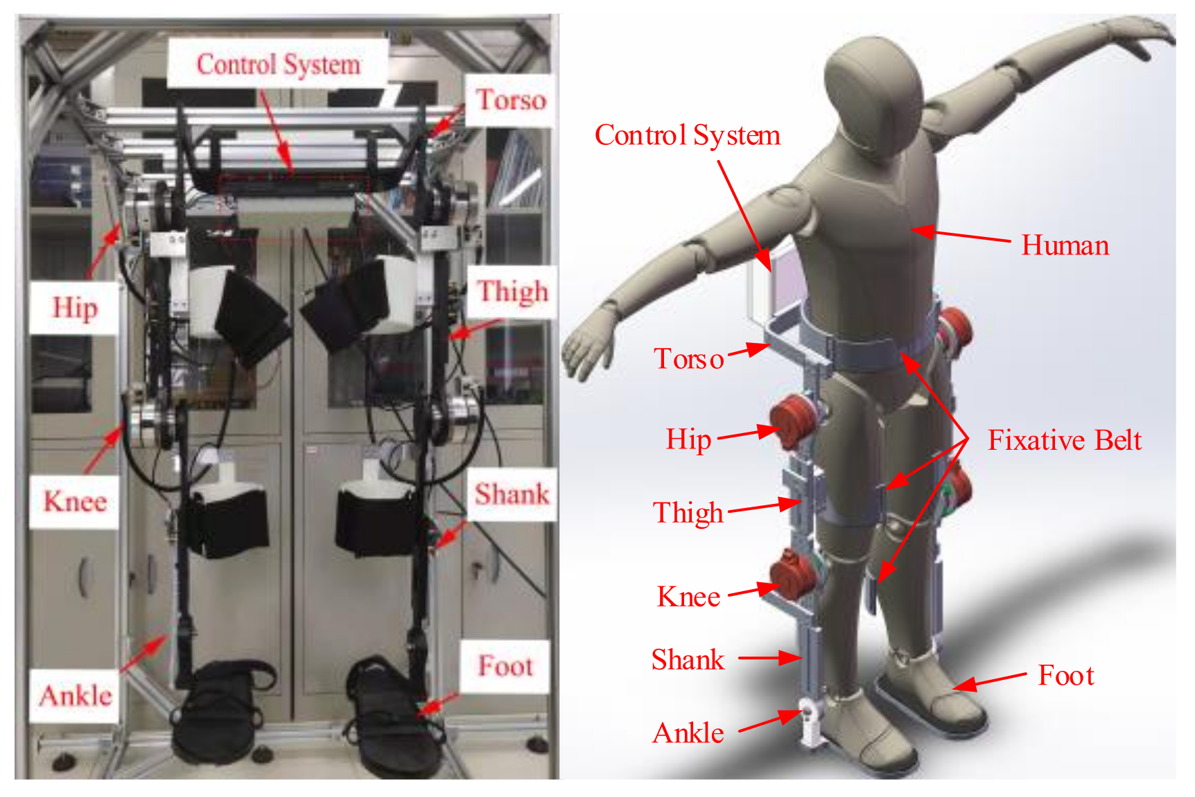
An adult male with a height of 1755 mm and a weight of 70 kg was selected as a representative patient for the lower limb rehabilitation exoskeleton robot. The patient and the robot were rigidly connected, and their movements were identical. As shown in
Figure 4, we utilized MATLAB/Simulink and RecurDyn dynamics software to build a human–machine coupling system simulation model.
The human-machine coupling system has five segments: the torso, the right thigh, the left thigh, the right shank and foot, and the left shank and foot. The parameters of each body segment are shown in
Table 3. Among these, the parameters of the right thigh and the left thigh were the same, and the parameters of the right shank and foot and left shank and foot were the same.
4.2. Simulation Parameters
The simulation time was 5 s, the simulation step length was 0.001 s, and the gait period was 2 s. The walking gait data of a normal person with a walking speed of 1.2 m/s was selected as the expected trajectory of each joint. The fitting curve is as follows.
where
is the desired trajectory of the right hip joint;
is the desired trajectory of the right knee joint;
is the desired trajectory of the left hip joint; and
is the desired trajectory of the left knee joint.
From Equation (21), the self-adaptive-coefficient double-power sliding mode control method proposed in this paper was recorded as SACDP-SMC. We set , , , , and the control parameter as the optimal parameter obtained after 120 online optimizations. , , , , , and .
To demonstrate the superiority of SACDP-SMC, we named it Method 1 and compared it with the following two control methods:
Method 2: To highlight the effect of the self-adaptive-coefficient , the double-power sliding mode control method was adopted and recorded as DP-SMC. The actual control torque of each joint of the robot is shown in Equation (13); the control parameters were the same as those described for SACDP-SMC.
Method 3: To highlight the compensation effect of the double-power sliding mode control, a traditional computed torque method based on PID was adopted, and recorded as PID-CTM. The actual control torque of each joint of the robot is expressed as follows.
where
,
, and
are control parameters of the computed torque method.
,
,
.
4.3. Simulation Results and Discussion
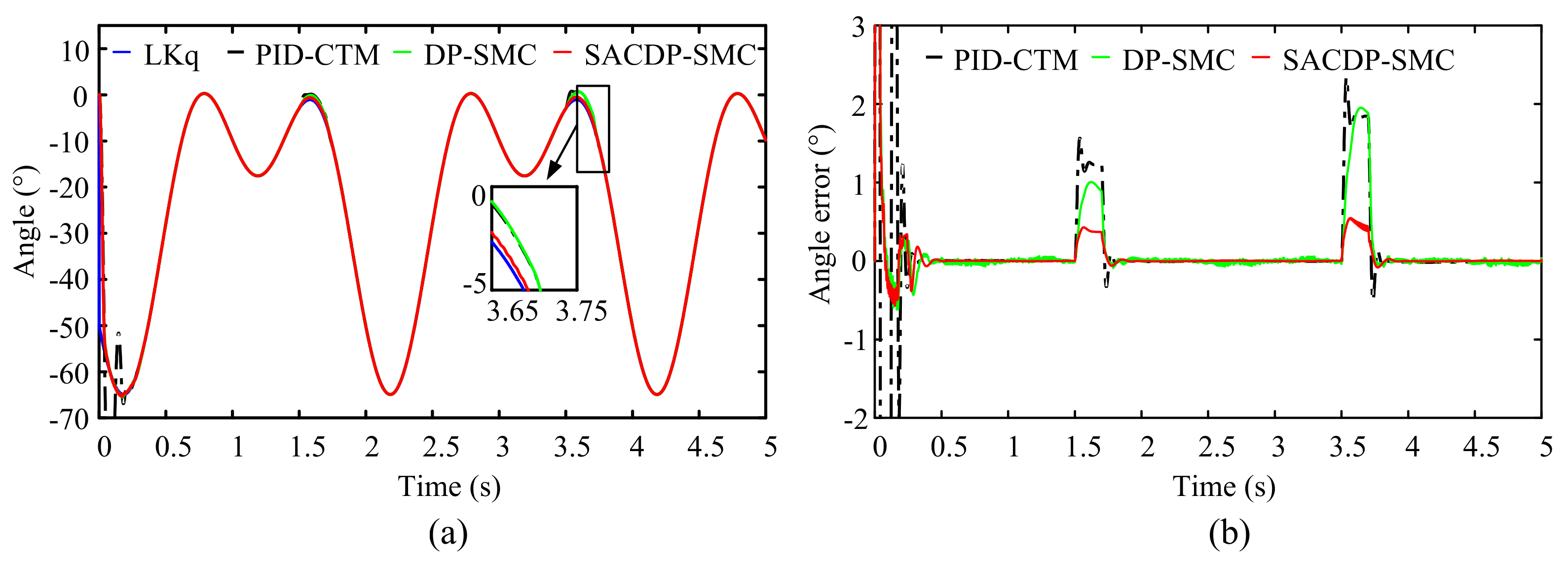
To compare the performances of the control algorithms, the patient’s interference with the lower limb rehabilitation exoskeleton robot was regarded as step interference. At 1.5 s and 3.5 s, and were applied to each joint of the robot for a duration of 0.2 s. These interferences also represent strong environmental interference to the lower limb rehabilitation exoskeleton robot.
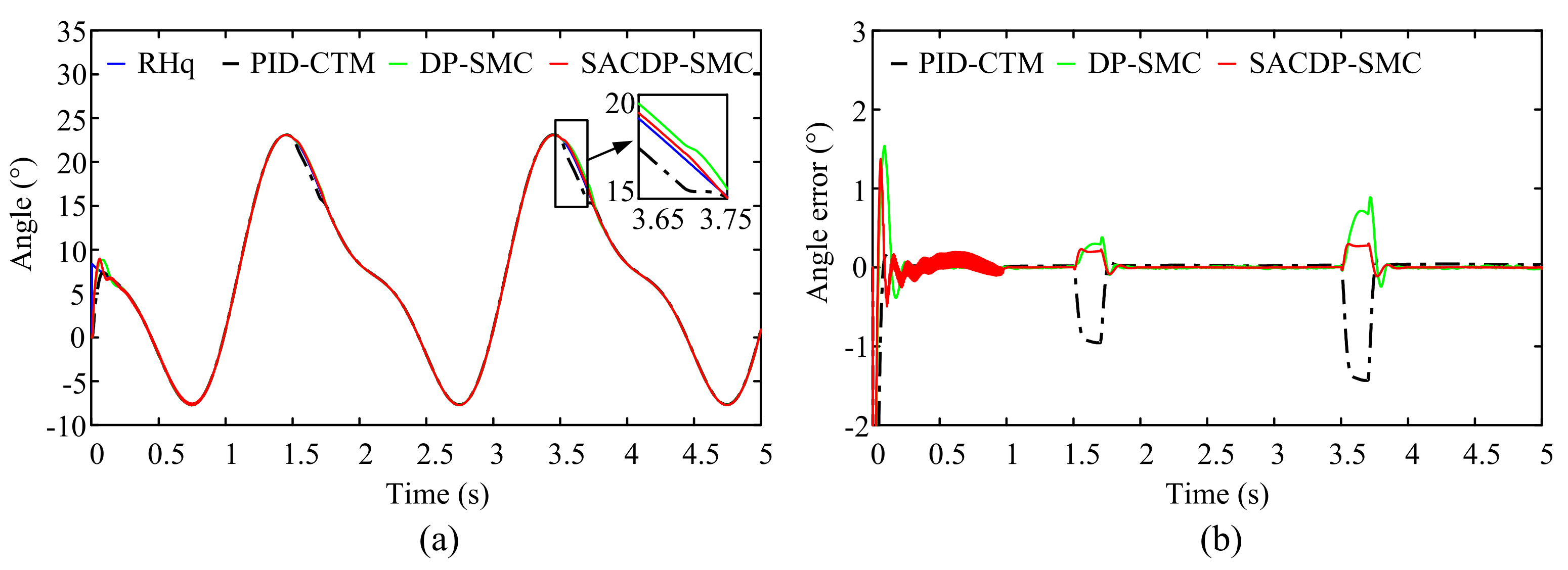
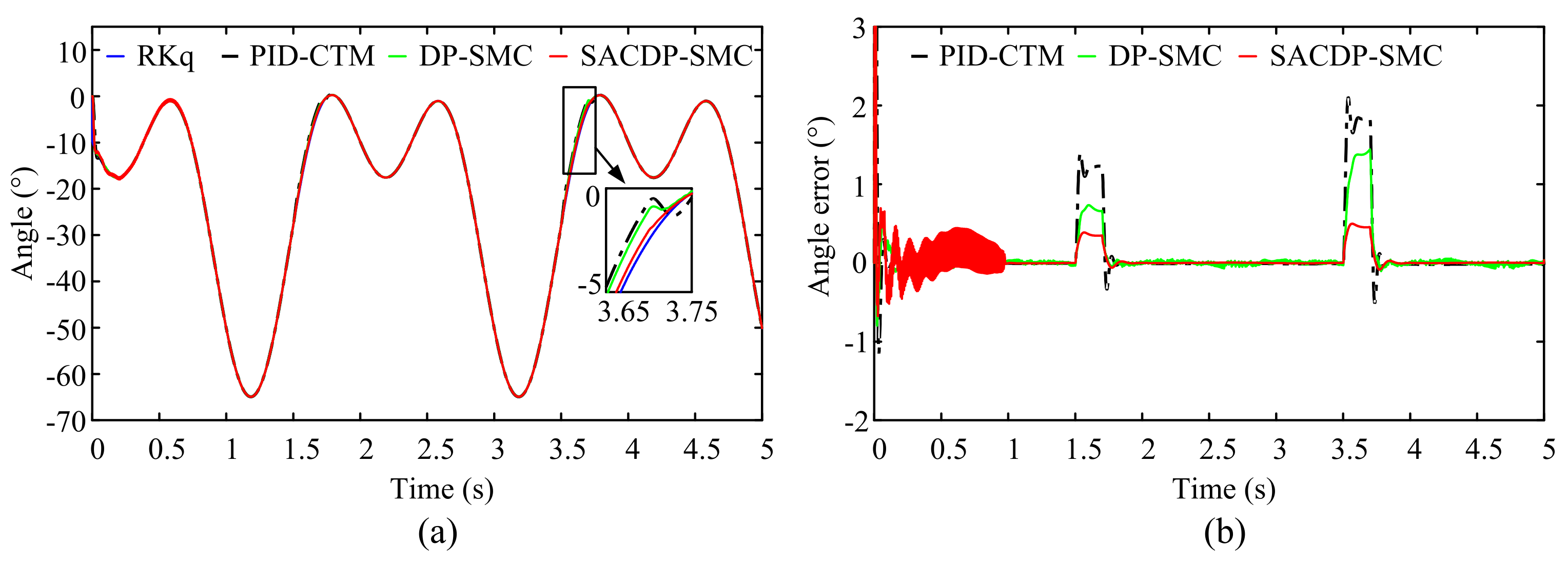
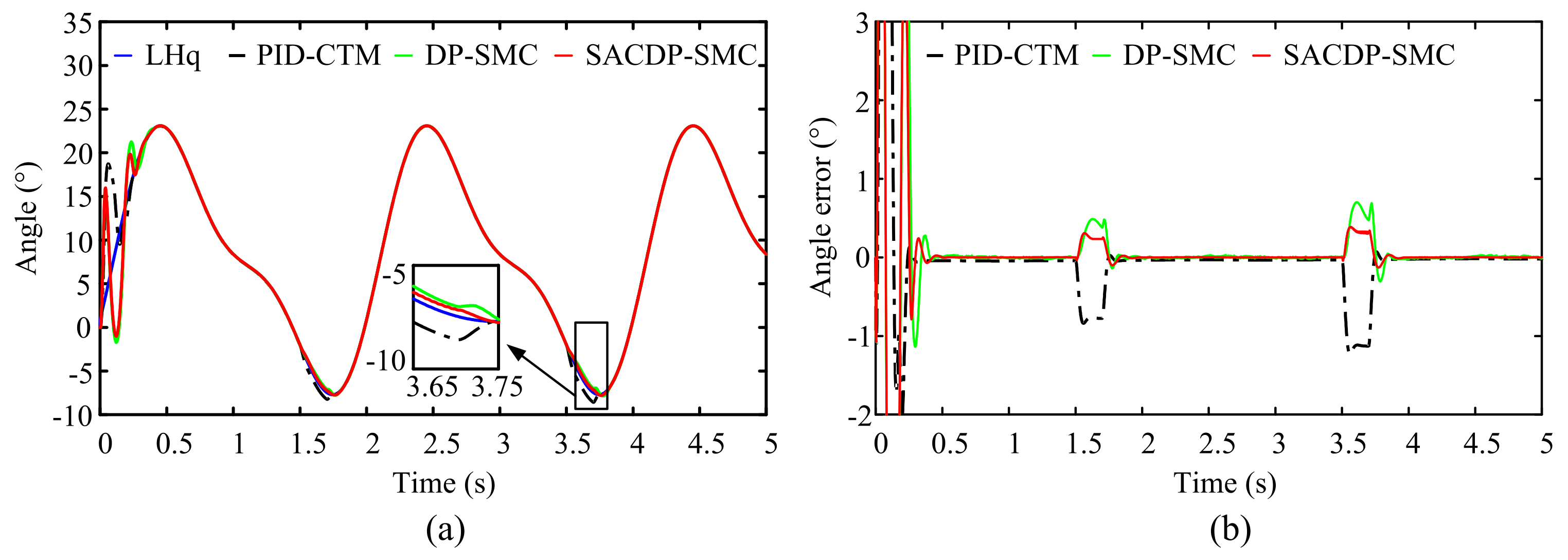
The trajectory tracking curve and tracking error curve of each joint of the lower limb rehabilitation exoskeleton robot are shown in
Figure 5,
Figure 6,
Figure 7 and
Figure 8. RHq, RKq, LHq, and LKq are the desired trajectories of the right hip, right knee, left hip, and left knee joints. All three control methods can achieve robot trajectory tracking to a certain extent, and the maximum tracking error occurs during the interference period. The following is a detailed analysis of the control accuracy and anti-interference performances.
To compare the control accuracy of the three control methods, the maximum absolute tracking error
, the average absolute tracking error
, and the root mean square error
were used as measurement indicators. When the control system is stable, the tracking error is calculated between 1 s and 5 s. The maximum absolute tracking error, average tracking absolute error, and root mean square error of the three control methods are shown in
Table 4. Compared with the errors when using the traditional computed torque, the percentage of tracking error reduction is shown in
Table 4.
In terms of
Table 4, it is clear that the maximum absolute error, average absolute error, and root mean square error of the DP-SMC were reduced by 16.54%, 15.54%, and 16.22%, respectively, compared with the PID-CTM under the interference of the patient. In addition, the maximum absolute error of the SACDP-SMC, the mean absolute error, and the root mean square error were reduced by 76.61%, 71.77%, and 73.44%, respectively. Both the DP-SMC and SACDP-SMC effectively reduce the trajectory tracking error and improve control accuracy, but the SACDP-SMC achieves the best control accuracy. Even if the patient simultaneously generates 75 Nm of interference torque on each joint of the robot, the maximum absolute error of the proposed SACDP-SMC was only 0.5474°.
Based on the maximum absolute error ; the average absolute error ; and the root and mean square error ; the SACDP-SMC proposed in this paper sharply reduced the trajectory tracking error of the lower limb rehabilitation exoskeleton robot and improved the control accuracy.
To compare the anti-interference capabilities of the three control methods, the error variation
and the interference adjustment time
were used as measurement indicators. Under patient interference, the maximum error variations of the three control methods are shown in
Table 5.
In terms of
Table 5, compared with PID-CTM, the maximum error variation of DP-SMC was reduced by 34.29% and 17.13%, and the maximum error variation of SACDP-SMC was reduced by 73.03% and 76.77%. Both the DP-SMC and SACDP-SMC effectively reduced the impact of interference, but the SACDP-SMC achieved the best anti-interference effect. When the patient simultaneously generated 75 Nm of interference torque on each joint, the maximum error variation of SACDP-SMC was 0.5425°.
Table 6 shows the adjustment times
and
of the three control methods for interference
and
. Compared with the PID-CTM, the maximum adjustment time of the DP-SMC was reduced by 16.61% and 14.46%, and the maximum adjustment time of the SACDP-SMC was reduced by 33.19% and 30.54%. Both the DP-SMC and SACDP-SMC effectively reduced the interference adjustment time and accelerated the error convergence speed, however, the convergence speed of SACDP-SMC was the best.
It can be seen from the error variation and the interference adjustment time that the proposed SACDP-SMC improves the anti-interference ability of the lower limb rehabilitation exoskeleton robot by a large margin.
4.4. Wearable Experimental Results and Discussion
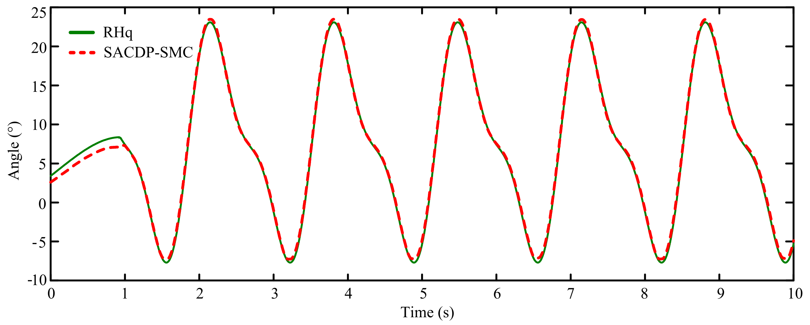
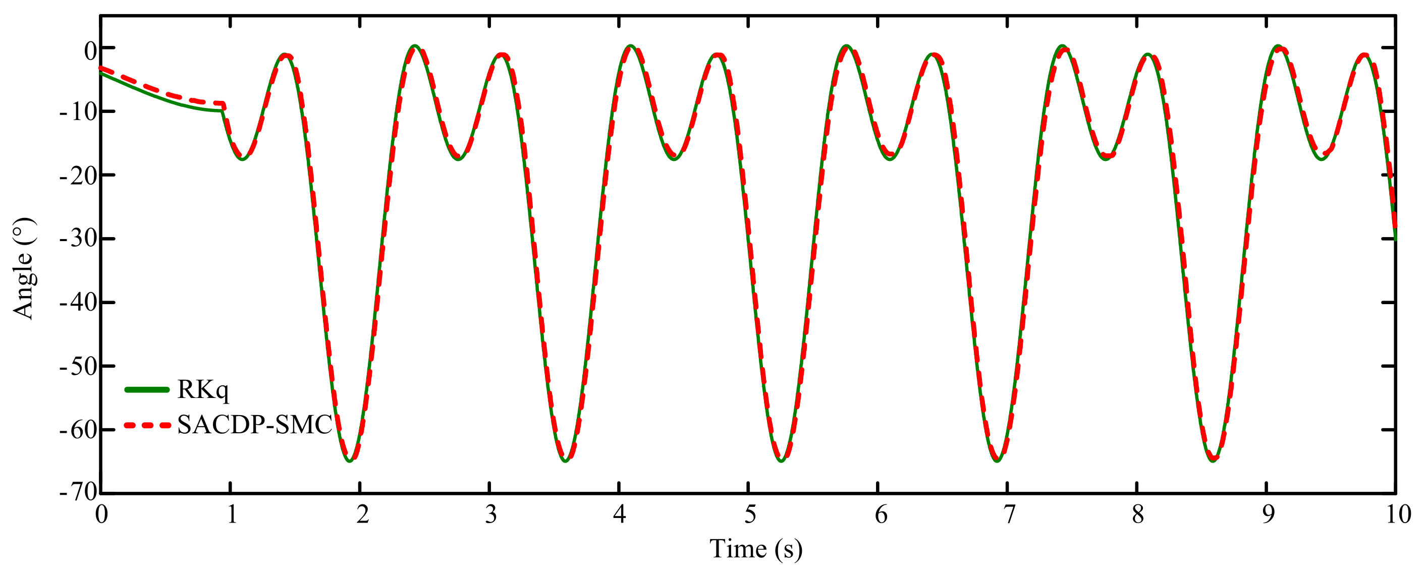
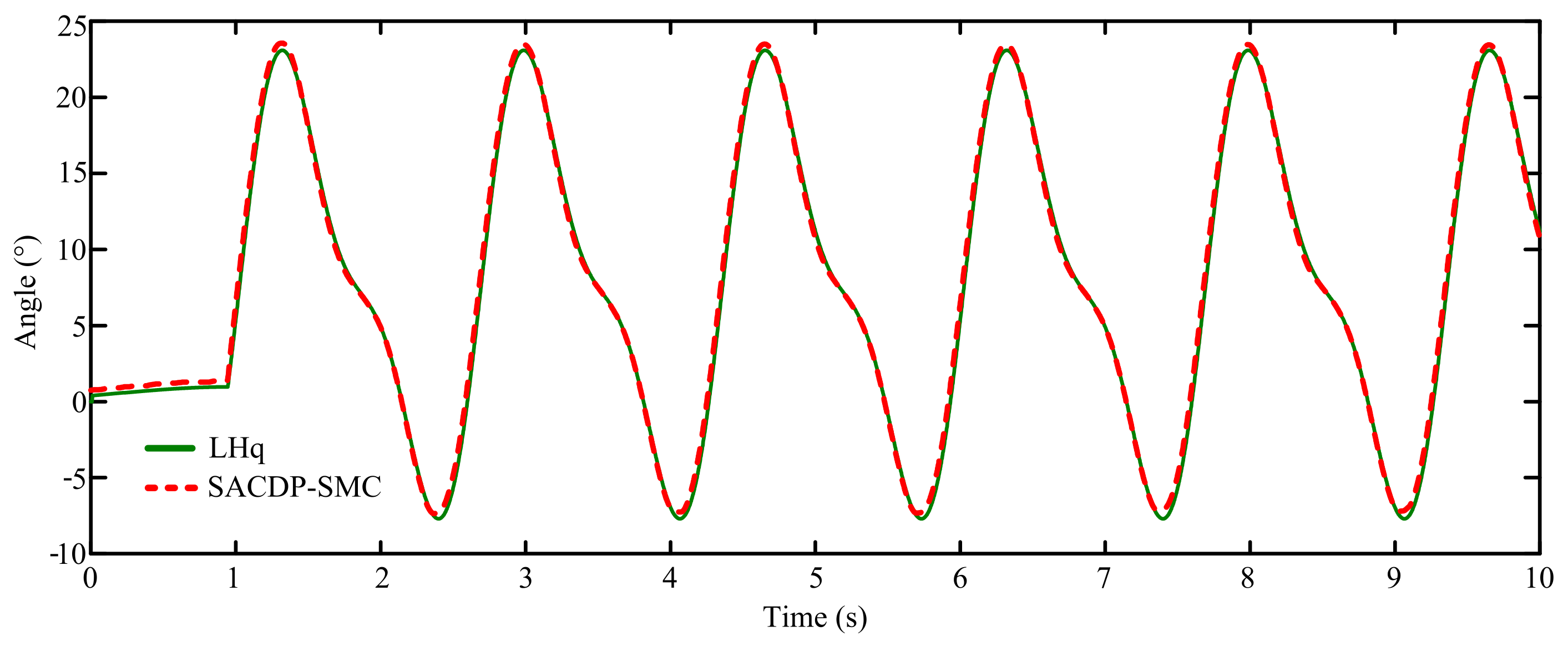
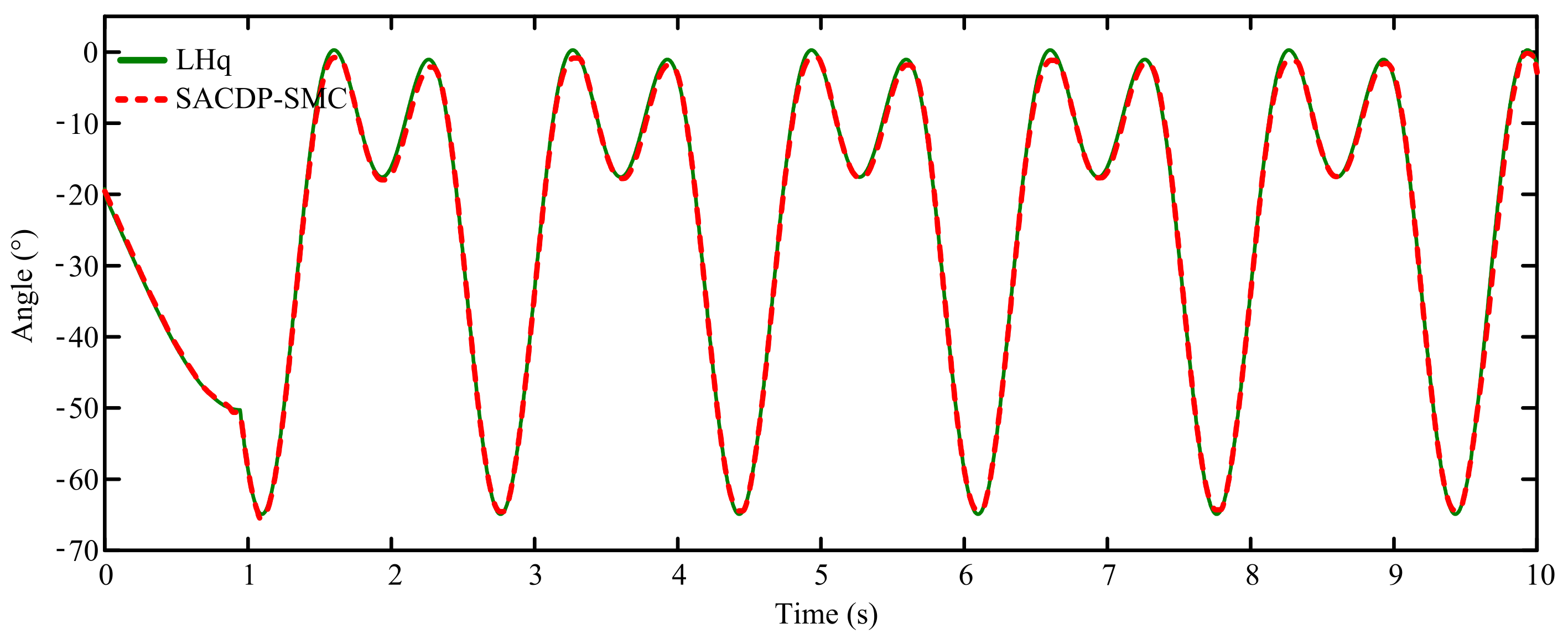
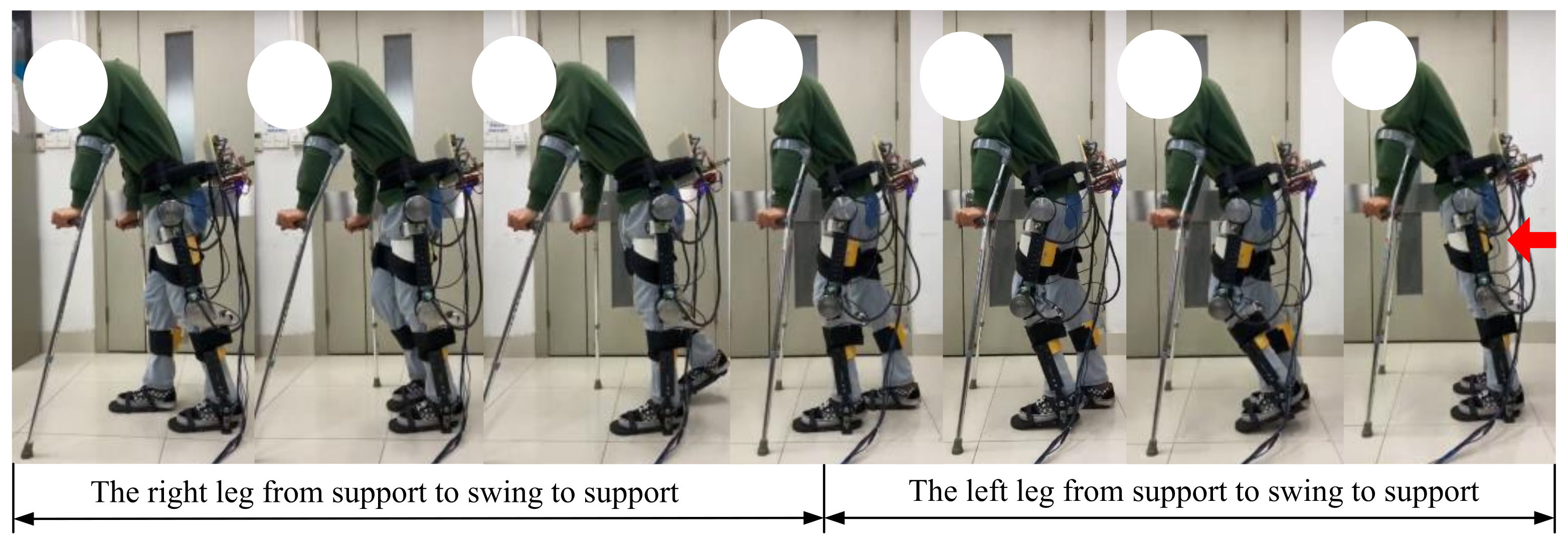
To verify the effectiveness of the self-adaptive-coefficient double power sliding mode control method, a wearable experiment was conducted on the lower limb rehabilitation exoskeleton robot prototype using selected healthy testers. The gait trajectory tracked by the lower limb rehabilitation exoskeleton robot still adopted the trajectory curve shown in Equation (21), and during the experiment, the lower limb of the tester was completely driven by the lower limb rehabilitation exoskeleton robot.
Figure 9 shows the seven intermediate motion states taken from the video of a complete gait cycle recorded in the experiment. The tracking trajectory curve of each robot joint is shown in
Figure 10,
Figure 11,
Figure 12 and
Figure 13, and the tracking error curve is shown in
Figure 14.
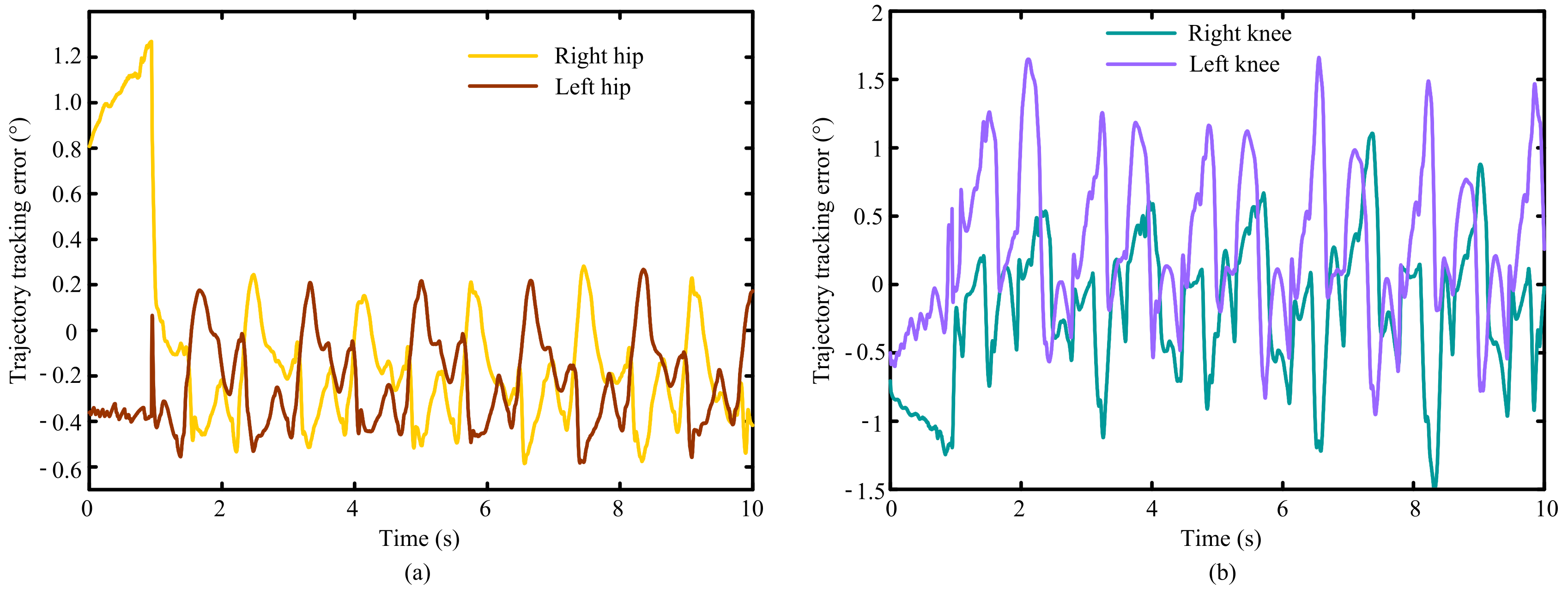
Figure 9,
Figure 10,
Figure 11,
Figure 12 and
Figure 13 show that based on the self-adaptive-coefficient double power sliding mode control method, the trajectory tracking error of the left and right hip joints ranged from −0.55° to 0.2°, and the trajectory tracking error of the left and right knee joints ranged from −1.5° to 1.65° when the lower limb rehabilitation exoskeleton robot prototype drives the tester to track the gait trajectory. Compared with the previous simulation results, the tracking error change of the hip joint was unobvious. The tracking error of the knee joint was increased, but it still had good tracking accuracy. Human gait movement was uncertain. Therefore, the movement of the tester wearing the lower limb rehabilitation exoskeleton robot can be regarded as a random disturbance. When the human wearing the exoskeleton carries out the gait experiment, the tracking error was very small. This shows that the self-adaptive-coefficient double power sliding mode control method proposed in this paper not only achieved good control accuracy, but also had good robustness. In this analysis, the tester was wearing the lower limb rehabilitation exoskeleton robot while walking on the ground, thus, when the legs were grounded, they were greatly disturbed by the ground, which increased the tracking error of the knee joint. In the follow-up research, we will deeply analyze the impact of the ground on the lower limb rehabilitation exoskeleton robot, establish the corresponding mathematical model, and design a controller with better performance.
5. Conclusions
In this article, a self-adaptive-coefficient double-power sliding mode control was proposed for trajectory tracking control of the lower limb rehabilitation exoskeleton robot. This method combines the estimated dynamic model of the robot and the sliding mode control based on the double-power reaching law. A nonlinear control law was designed based on the dynamic model of the robot and the method of calculating torque. The compensation term of the control law was introduced and the self-adaptive-coefficient of the compensation term of the control law was designed to reduce the interference of model error and environmental factors and improved the anti-interference ability of the robot.
Simulation analyses of the self-adaptive-coefficient double-power sliding mode control method, the double-power sliding mode control method, and the traditional computed torque method were performed. The results show that the self-adaptive-coefficient double-power sliding mode control method greatly improved the trajectory tracking accuracy and anti-interference ability.
The simulation showed that the self-adaptive-coefficient double-power sliding mode control method could reduce the trajectory tracking error by more than 71.77% compared with the traditional computed torque method. Even under strong environmental interferences (50 Nm and 75 Nm), the maximum absolute tracking error of the robot remained below 0.5474°. The wearable experiment shows that the lower limb rehabilitation exoskeleton robot had good robustness, and the maximum absolute error of the hip joint and knee joint remained below 0.55° and 1.65°, respectively.


 ,
, 


