Micro Activities Recognition in Uncontrolled Environments

Abstract

Deep learning has proven to be very useful for the image understanding in efficient manners. Assembly of complex machines is very common in industries. The assembly of automated teller machines (ATM) is one of the examples. There exist deep learning models which monitor and control the assembly process. To the best of our knowledge, there exists no deep learning models for real environments where we have no control over the working style of workers and the sequence of assembly process. In this paper, we presented a modified deep learning model to control the assembly process in a real-world environment. For this study, we have a dataset which was generated in a real-world uncontrolled environment. During the dataset generation, we did not have any control over the sequence of assembly steps. We applied four different states of the art deep learning models to control the assembly of ATM. Due to the nature of uncontrolled environment dataset, we modified the deep learning models to fit for the task. We not only control the sequence, our proposed model will give feedback in case of any missing step in the required workflow. The contributions of this research are accurate anomaly detection in the assembly process in a real environment, modifications in existing deep learning models according to the nature of the data and normalization of the uncontrolled data for the training of deep learning model. The results show that we can generalize and control the sequence of assembly steps, because even in an uncontrolled environment, there are some specific activities, which are repeated over time. If we can recognize and map the micro activities to macro activities, then we can successfully monitor and optimize the assembly process.

1. Introduction

Assembly of the machines in industries is a complex process. These processes involve the tiny components which increase the ratio of error during the process in case of any forgotten part, which is required to be inline. Sometimes the whole process has to be reversed. The worker working on these assembly processes needs to bring hundreds of different components and screw them with each other. Multiple workers need multiple hours to assemble one ATM, which is laborious and time taking. After assembly of the whole ATM, if a worker has forgotten even a single screw, then it would not work properly. Workers must disassemble the whole ATM which will again take hours to fix the missed component. Hence, the whole process is complex. This is the normal tendency that a human makes mistakes in complex industrial environments. Another important factor which is improved is lean manufacturing. Lean manufacturing is a concept in which using managerial or monitoring techniques, we improve the productivity of the existing systems. The main motto of lean manufacturing is efficient and cost-effective output with ultimate client satisfaction [1]. In this paper, we will explain the problem specific to the ATM assembly process. To find the solution for this problem and to make the process optimized and efficient, in this article, we will suggest a modified deep learning network. Deep learning [2] is a domain of artificial intelligence (AI) that mimics the workings of the human brain in processing and analyzing patterns. Deep learning has proven very efficient for object detection, speech recognition, language translation and for general decision making processes. The horizons of deep learning are as vast from the aeroplane [3] automation control to the simple character recognition [4].

Our Approach

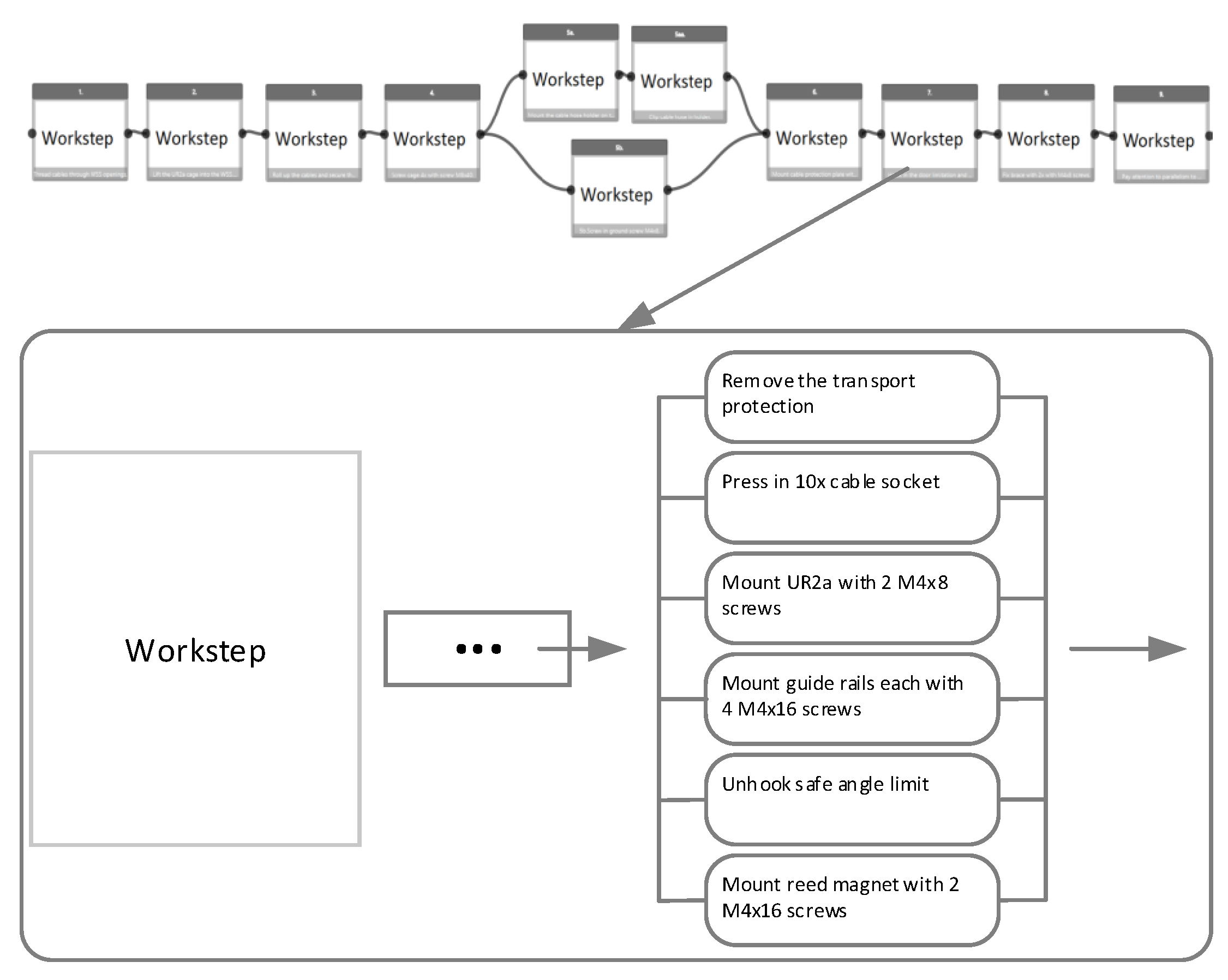
In this work, our goal is to observe and recognize the pattern of the screwing activities, from the egocentric view of the worker. For this purpose, we have recorded the data from the pupil platform (https://pupil-labs.com/ accessed on 2 November 2021) eye tracker’s word camera. In our case, there are four different types of screwing activities which involve different work steps. We make a hierarchical division of activities, by dividing the whole process into macro and then micro work steps, where in each micro-work step, there are different screwing activities. An example of this division is shown in Figure 1 below. There are four different main activities which must be detected and classified so that micro-level work steps are accurately completed.

There are many different techniques in the literature for human action recognition. However, the assembly action recognition is different than human action recognition. In assembly action recognition, there are many different working tools involved, which play an important role in detecting and recognizing the assembly action. For example, Chen et al. [5] presented the study to control the mistakes made by workers by recognizing the commonly repeated actions in the assembly process. The YOLO-V3 [6] network was applied for tools detection.

We used deep learning technology to monitor the assembly process and guide the worker, working on the ATM assembly. We identified the activities performed by the workers to increase the quality of work. Therefore, assembly action recognition is the issue which will be resolved in this research, especially related to the ATM assembly steps which include multiple different screwing activities.

To examine the proposed approach for detecting the micro activities as presented in Figure 1. There are three main stages, including data collection, data prepossessing and classification of the actives. For the classification stages, we have used four different models to compare and enhance the results which are described and discussed in details in Section 3. Section 2 explain and discuss the previous research work related to our problem. Data collection and the data preparations for our proposed classifiers are mentioned in Section 4. Results of our classifiers are presented in Section 5 and detail discussion of results are discussed in Section 6. In the end, We closed with a short conclusion in Section 7.

2. Related Work

The timeline, history and unprecedented achievements of AI are described in the paper of Venkatasubramanian [7]. It unfolds the story of more than three decades to improve industry production using AI. Deep learning is a sub-branch of AI and machine learning. Deep learning has been implemented successfully in many applications. Deep learning was also introduced for the assembly process control and management [8]. The researcher monitored the process in two steps. In the first step, using the fully convolution network (FCN), the model recognizes the action of the worker. At the second step, the parts to be assembled are recognized. These parts are sometimes very small in size. For action recognition, as a base network, the convolution neural network (CNN) was used with three dimensions. Additionally, the image normalization is also performed for the identification of any missing parts.

Such a type of assembly control project is used to monitor and automate the sequence of human actions in the assembly of hardware by Wang et al. [9]. In his study, the researcher used the temporal segment network (TSN) technique. Basically, the TSN is a two-stream CNN. His work is primarily related to action recognition based on video clips. TSN uses colour difference with the input of the optical flow graph. Feichtenhofer [10] suggested a modified CNN fused with two-stream networks. These networks are used for action detection in images and videos. In fusion, CNN towers are used as temporally and spatially. Feichtenhofer, who takes the single frame as input for the CNN using a spatial stream, along with temporal stream as the input for optical flow based on multi frames. These spatial and temporal streams are then fused by a filter. This is a 3D filter with the ability to mature its learning based on communication among the features of temporal and spatial streams. A three-dimensional CNN is created by Tran [11], which is named as C3D. This approach extracts the spatial-temporal features for learning using deep 3D-CNN [12].

Du [13] suggested the recurrent pose-attention network (RPAN). A full recurrent network was being used by RPAN. The method is based on the mechanism of postural attention. This model has the ability to extract and learn human motion features by exploiting the parameters of human joints. The motion features which are extracted using this technique are then fed into the aggregation layer. The layer ultimately builds the positional posture representation for temporal motion modelling. Task recognition is also performed by using long-term recurrent CNN (LRCN). This is proposed by Donahue [14]. In this technique, he used sensors to extract the required features in the time sequence. Then, he used this time series as input to the long short-term memory (LSTM) network, which is able to perform the classification in an enhanced efficient manner.

Region convolution 3D network (R-C3D) also showed promising performance for task detection and sequencing. This model was proposed by Xu et al. [15]. In R-C3D, they first measure the features using the network. Then, to ensure the sequence of tasks in the required manner, they obtained the time-related areas, which might have relevant activities in accordance with the features of R-C3D. In the end, they detect the actual activities in those areas, which are related to R-C3D recommended area and features. The R-C3D has the great ability to manage both short and long length videos as input. Illumination is one of the key factors for task recognition. The variations in illumination intensity lead to different meaningful features. To be focused on assembly process sequence, it is important to minimize the environmental effects which lead to changes in illumination. Minimized illumination variations significantly improve the accuracy and performance of the model. Khaleghi in his paper [16] analyzed the accuracy and speed of neural network training based on the effects of binary, grey and depth images. A CNN model was designed, which is three-dimensional and serves the dimensional information as the input to the model. This model uses the techniques of single channel gray video sequencing. The CNN model is further improved by the induction of an additional layer, the core purpose of this layer is to normalize the batch which will be used as input to the model. This approach enhances the overall performance of the network. It is also revealed in this paper that no information is lost in the case of the conversion from RGB images to single channel grayscale images. The model learns the same features in both dataset formats, but in the case of single-channel, the size and efficiency of the model in terms of time are improved. However, the important factor to remember is that the sensitivity is reduced in the case of single-channel grayscale images to different illumination conditions.

C3D [11], two-stream CNN [17], LRCN [18] and LSTM are the most commonly used models for motion detection. [11] applied all these four models to the publicly available datasets UCF-101 [19]. The comparison shows that all models have approximately similar accuracy levels but the time efficiency of C3D is better as compared to others reaching higher frames rate per second. On the other hand, the earlier two-stream model executed only 1.2 frames per second [10]. The reason for this variation of frames per second is due to simple network structure and efficient data pre-processing of C3D model. The two-stream model first processes image sequence and along with that it also extracts the optical flow information, which ultimately slows down its performance due to these mentioned layers. Being multi-layered, parallelism has to be implemented for the recurrent neural network (RNN); this parallelism makes the RNN model complicated and computationally expensive. Other methods mentioned in the literature show that 3D-CNN model is comparatively more suitable due to its structure for the control of assembly process monitoring and management because of its less complicated structure. Other features of 3D-CNN include less training time with high accuracy. These features make this 3D-CNN fittest for industrial control and monitoring applications.

Since the semantic segmentation is an option in three dimensional CNN, in which each pixel is categorized into different classes. For this purpose, each pixel is analyzed which makes it more refined and accurate. Another approach for pixel-level classification is made by Shotton et al. [20]. They used pose estimation for the detection and classification of objects and action detection. Depth information increases the accuracy in action recognition as the movement in different directions is detectable for high accuracy results. The extracted depth maps are further utilized for the pixel level matching for different types of objects and even for different instances of the same object. Joo et al. [13] suggested another unique method for the detection of the hand region. Based on depth maps for all types of objects, their proposed method identifies the hand region in real-time using the feature of depth maps. Another semantic segmentation technique proposed by Long et al. [21], which is based on FCN as the FCN, has proven to be the deep learning cornerstone for solving the detection and classification tasks. Ronneberger et al. [22] proposed U-Net network based on encoder and decoder. In the encoding process, the network extracts contextual features, and in the decoding phase, maps the symmetric recovery target. This U-Network has a feature which allows it to use small datasets as training and produce accurate feature maps of these small datasets. They implemented this network on biomedical imaging with high accuracy. The pyramid scene parsing network (PSPNet) was presented by Zhao et al. [23]. In this model, they implemented the function of global context information capturing by fusing the directional information. PSPNet is the appropriate option for this fusion. The PSPNet also proved to be efficient in scene analysis tasks. How much effective is the role of kernels using multiple levels was explored by Peng et al. [24]. The model was specifically designed to face the parallel segmentation and classification tasks and to propose a global optimized CNN which expands the receptive fields using atrous convolution without reducing the resolution. Deep learning techniques were also successfully used in different types of other industrial applications by Fu [25], Carvalho et al. [26], Iglesias et al. [27], Li et al. [28] and Kholief et al. [29].

At the end of this related literature review, it is also important to mention that the dataset we used was generated in an uncontrolled environment. The datasets are not synthetic and also not created in controlled environments. This uncontrolled environment feature of our dataset has important effects for selection and design of neural network models for our research. We can conclude that all the applications which are based on images or videos, where the depth of different images matter, CNN architecture is best suited. CNN is also being implemented successfully in biomedical imaging for segmentation purposes, for scene analysis in traffic control and surveillance applications, for face classification in social media and other applications, and so on. The use of CNN in assembly line process management is still a challenging task, due to the complexity of scene analysis and many other factors. Assembly process management comparatively has huge possible cases for even a single action due to the difference in human working styles. In assembly process management, controlling the sequence of steps and detection of errors and mistakes made by humans is very hard due to the nature of assembled parts. Sometimes, the parts are so tiny and barely visible to detect during the assembly. Assembler’s hand occlusion is another issue. Such scenarios demand entirely new approaches to tackle the problem. All the techniques that we found in the literature review are summarized in

Table 1. Summarized table of literature review.

Ref. No.	Year of Publication	Technique	Findings
[9,10]	2016, 2016	FCN, TSN Two stream CNN Spatio-temporal features	Action recognition in videos. Temporal segment network (TSN) based longrange temporal structural modelling based on two-stream CNN.
[8,11,12]	2020, 2015, 2012	3D-CNN	Full convolution neural networkfor action Detection. Three dimensional CNN with batch normalization for missing parts Identification. Decision making is also based on spatial-temporalfeatures.
[13]	2017	Recurrent pose-attentionnetwork (RPAN)	The method is based on the mechanism of postural attention.  Extracts the features of motion using human jointsinformation.
[14]	2018	LSTM	Detects features using sensors and then classifying using LSTM. The time sequence is used to detect the missing parts.
[15]	2011	Region Convolution 3DNetwork (R-C3D)	Action recognition using time sequence of activities during thetraining. Ability to manage short and long videos. Illumination variations were also used as features.
[16]	2013	CNN	Analyzed the accuracy and speed ofneural network training based on the effects of binary, grey images with depth information. Increase in performance efficiencydue to image batch normalization. In the case of single channelimages, important information about intensity is affected. Parallel processing of layers formulti kernel approach Kernels are changed by changing the size of the receptivefield size.
[20,21,22,24]	2013, 2017, 2015, 2017	CNN Semantic image segmentation	Pixel level classification usingsemantic image segmentation. Use of different types of kernels on a different levelof network layers.
[23]	2017	Pyramid scene parsing network (PSPNet)	The decision is based on globalcontext information. Global context information isgenerated using directional information. Efficient for the scene analysis task.

.

3. Classification Methods

We used four different state of the art deep learning networks. Out of the four networks, the two main networks are Inception-V3 (Google, Mountain View, CA, USA) and the VGG-19 (MathWorks, Portola Valley, CA, USA). The reason behind selecting these two networks is that there are many different deep learning networks available, but these two methods are proven to have a comparatively high accuracy rate [30]. Inception-V3 has high accuracy with a smaller number of operations. VGG-19 has a higher number of operations and has an acceptable accuracy rate. Comparison of different deep learning networks done in [30]: Top-1 accuracy vs. operations size is being compared, the VGG-19 have around 150 million operations, and operations size is proportional to the size of the network parameters. Inception-V3 shows promising results and has a smaller number of operations as compared to VGG-19. That was the motivation to choose these two networks for our research. Inception-V3 has high accuracy with a smaller number of operations. VGG-19 has a higher number of operations and has an acceptable accuracy rate, as the comparison of these networks can be seen in Figure 2.

The third and fourth networks are two-stream CNN and Inception-V3 with the blend of LSTM respectively. These third and fourth networks are built on top of the previous two networks. One network we have combined is the Inception-V3 and VGG-19 with the LSTM. LSTM is proven to be best when it comes to mapping the sequence over time. The fourth network was the two-stream network, where we have used two Inception-V3 networks working in parallel which will be described in detail in Section 3.2. These networks are widely used in deep learning. The purpose of the multi-network approach is to check the suitability of the network, particularly for our problem in terms of accuracy and high precision.

3.1. Inception-V3 and Visual Geometry Group—19 (VGG-19)

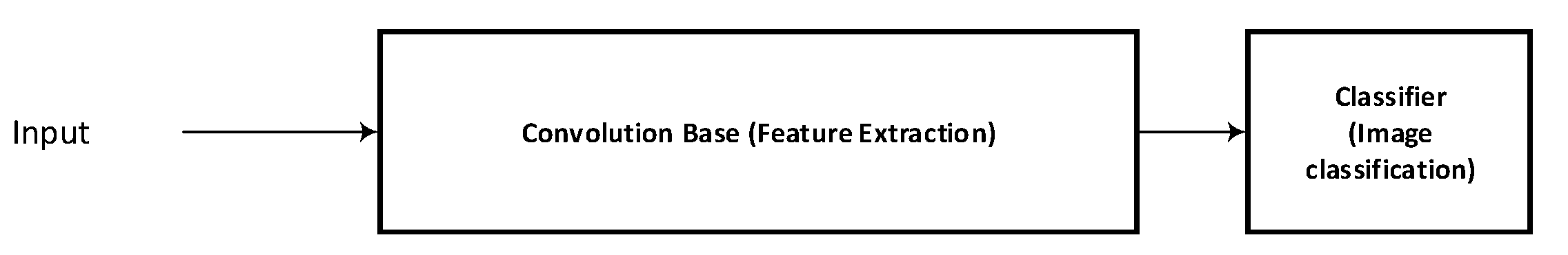
Inception-V3 [31] is based on CNN and used for large datasets. Inception-V3 was developed by Google, and trained on the ImageNet’s (http://www.image-net.org/ accessed on 2 November 2021) 1000 classes. Inception-V3 contains a sequence of different layers concatenated one next to the other. There are two parts in the Inception-V3 model, shown in Figure 3.

3.1.1. Convolution Base

The architecture of a neural network plays a vital role in accuracy and performance efficiently. The network used in our experiments contains the convolution and pooling layers which are stacked on each other. The goal of the convolution base is to generate the features from the input image. Features are extracted using mathematical operations. Inception-V3 has six convolution layers. In the convolution part, we used the different patch sizes of convolution layers which are mentioned in

Table 2. Inspection-V3’s architecture used in this paper [31].

Layer	Patch Size/Stride	Input Size
Conv	3 × 3/2	224 × 224 × 3
Conv	3 × 3/1	111 × 111 × 32
Conv padded	3 × 3/1	109 × 109 × 32
Pool	3 × 3/1	109 × 109 × 64
Conv	3 × 3/1	54 × 54 × 64
Conv	3 × 3/1	52 × 52 × 80
Conv	3 × 3/1	25 × 25 × 192
Inception A × 3	-	25 × 25 × 288
Inception B × 5	-	12 × 12 × 768
Inception C × 2	-	5 × 5 × 1280
Fc	51,200 × 1024	5 × 5 × 2048
Fc	1024 × 1024	1024
Fc	1024 × 4	1024
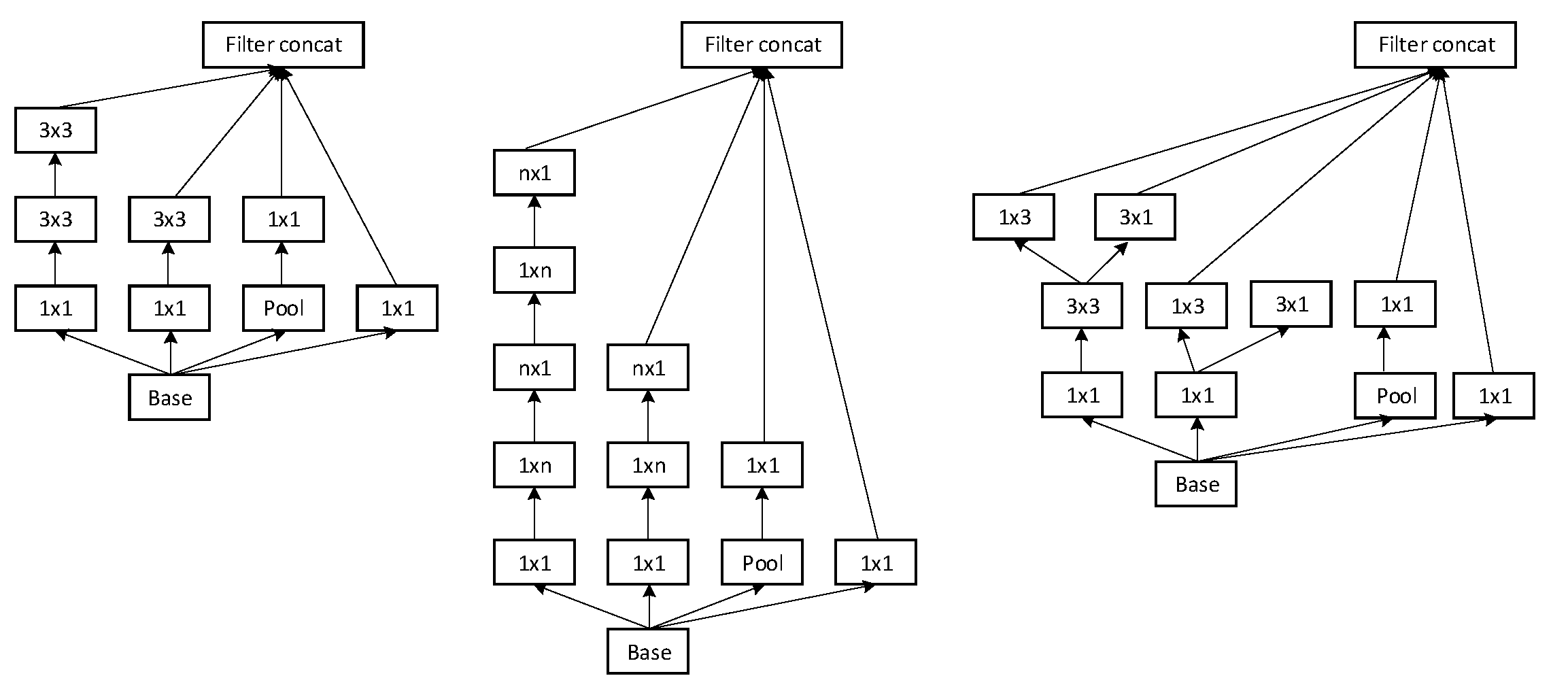
SoftMax	Classifier	4

. There are three different types of Inception modules shown in Figure 4. Three different inception modules have different configurations. Originally, inception modules are the convolution layers which are arranged in parallel pooling layers. It generates the convolution features, and at the same time, reduces the number of parameters. In the inception module, we have used the 3 × 3, 1 × 3, 3 × 1, and 1 × 1 layers to reduce the number of parameters. We used the Inception module A three times, Inception module B five times and Inception module C two times, which are arranged sequentially. By default, image input of inception V3 is 299 × 299, and in our data set, the image size is 1280 × 700. We reduced the size to the default size, keeping the channels number the same and changing the number of feature maps created while running the training and testing.

3.1.2. Classifier

After convolution layers and Inception modules A, B and C, the feature maps were 5 × 5 × 1 with 2048 channels. After this, we added one fully connected (FC) layer at the end of the Inception-V3 model. These layers will use the convolved features to make a prediction. Inception-V3 allows us to utilize the pre-trained model and fine tune the parameters for our own classification task. After the FC layer, SoftMax layer was added for the probability calculation of classes.

The main feature is to classify the image based on the extracted features. These are the FC layers where the neurons of the layer are fully connected to the previous layer.

Similar to Inception-V3, we have implemented the VGG-19 [32] pre-trained model, which initially was used with the single frame process and analysis. VGG-19 is also the network which was trained on the ImageNet dataset. It contains 16 CNN layers.

3.1.3. Transfer Learning with Pre-trained Convolution Networks

The method of transfer learning [33] with pre-trained deep convolution networks consists of two main parts: The construction of pre-trained convolution networks and the fine-tuning phase as shown in Figure 5. We have frozen the convolution base part of the model which was trained on the ImageNet images. We have retrained the classification part which has fully connected layers and SoftMax function. With the help of the transformation technique, we can use the model to our classification part, because the convolution part provides the convolved features. We pass these features to the classification part of the network. We retrain the last classifier part of the convolution network with our own classes instead of the 1000 classes of ImageNet dataset. In our use case, we have five different classes. The use of pre-trained models called the transfer learning is used in different applications, such as real-world simulations [34], gaming [35], image classification [36,37,38], zero shot translation [39] and sentiment classification [40], etc.

3.2. Two-Stream CNN

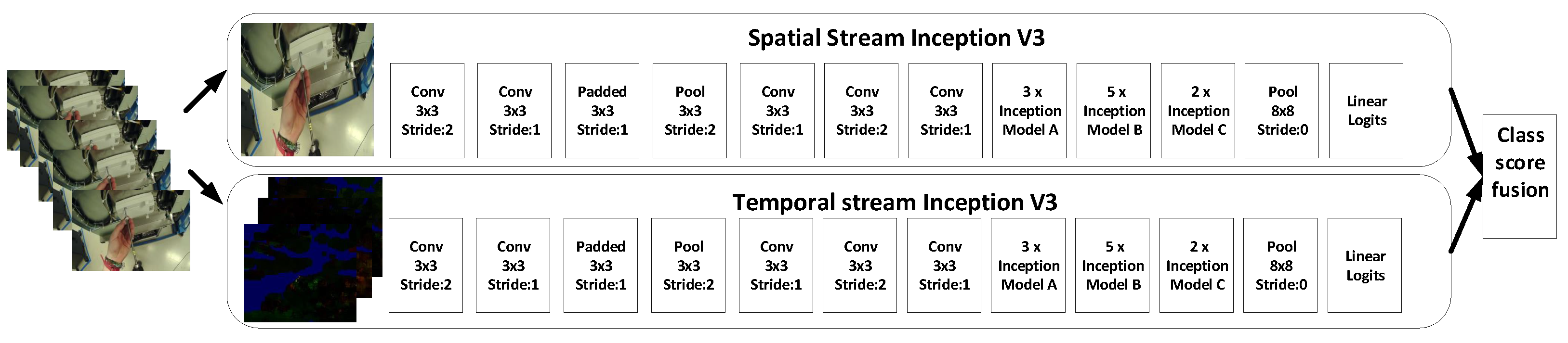
The second method used in this paper is the two-stream CNN [41]; it is the extension of state of the art CNN. In the two-stream method, we used two Inception-V3 models, where one will be working as spatial stream CNN and second will be working as a temporal stream CNN, as can be seen in Figure 6. The Inception-V3 used in this method will be similar as described in the previous Section 3.1. We used spatial stream CNN to perform action recognition on the single still frame. Some actions are particularly associated with some objects, hence this could be useful. Spatial stream CNN is an image classification architecture, we used the pre-trained network trained on the ImageNet dataset. Next section will describe the temporal stream CNN, which will use motion between the frames to improve the accuracy.

The layer configuration of the two-stream network in Figure 6. Spatial stream CNN is similar to Table 2. We used the ReLU rectification [42] for all the hidden layers. The main difference between the spatial CNN and temporal CNN is that we have removed the second normalization layer from the temporal CNN to reduce the memory consumption. We used the stochastic gradient descent [43] for the training of the network. At every iteration batch of 128 video samples from the training set, from each of these videos, a single frame is randomly selected. Training of the spatial CNN is a sub-image of 299 × 299 randomly cropped from the selected frame. In the temporal CNN training, we computed the optical flow of the selected frames as it is described in detail in Section 4.

Optical Flow Calculating the optical flow, a minimum of two frames are required to calculate the motion flow between the frames. Hence, given the two frames, we come up with a 2-dimensional vector which is called the optical flow vector. It gives the displacement of each of the pixels compared to the previous frame. That vector tells how much the specific pixel moved as compared to the prior frame. We will compute the optical flow from Lucas and Kanade’s equation described in detail in Section 4.

3.3. Combination of CNN with RNN (LSTM)

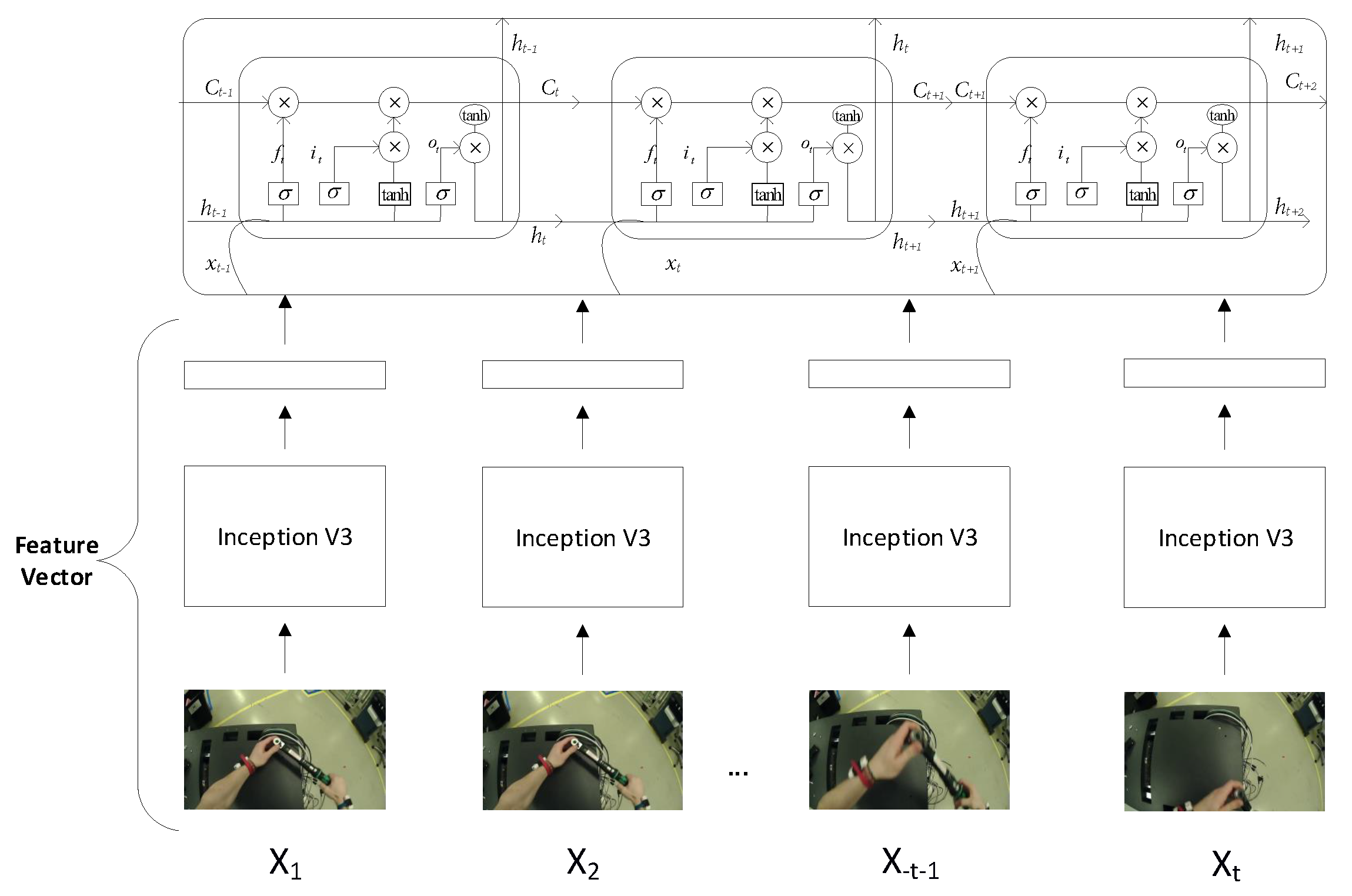
A method in which we have combined two models: the Inception-V3 and RNN (LSTM). CNN obtains hidden unique patterns in images; it depicts all the little changes in each frame. These changes in sequential form are learnt through RNN for action recognition in a stream of the frames. We will obtain features of images, obtained from the avg_pool neuron layer of the Inception-V3 model. We will extract the features of each frame with a sequence. These sequences will serve as input to the LSTM network. LSTM network performs well on sequence datasets. The LSTM network can analyze the current frame and remember the state of previous frames. The architecture of the combined models can be seen in Figure 7.

LSTM is the cell which is used in the RNN. RNNs suffer from the vanishing gradient problem. LSTM plays a roll in solving the vanishing gradient problem, and had been used widely for the time series analysis. Figure 7 showed how the LSTM cells are at each time step. $X_1,X_2,...,X_t$ input states of the LSTM. $C_1,C_2,...,C_t$ are the cell states and hidden states are $h_1,h_2,...,h_t$. $f_t,i_t$ and $o_t$ are the forget, memory and output gates of CNN/LSTM, respectively. Details can be read [44].

4. Dataset

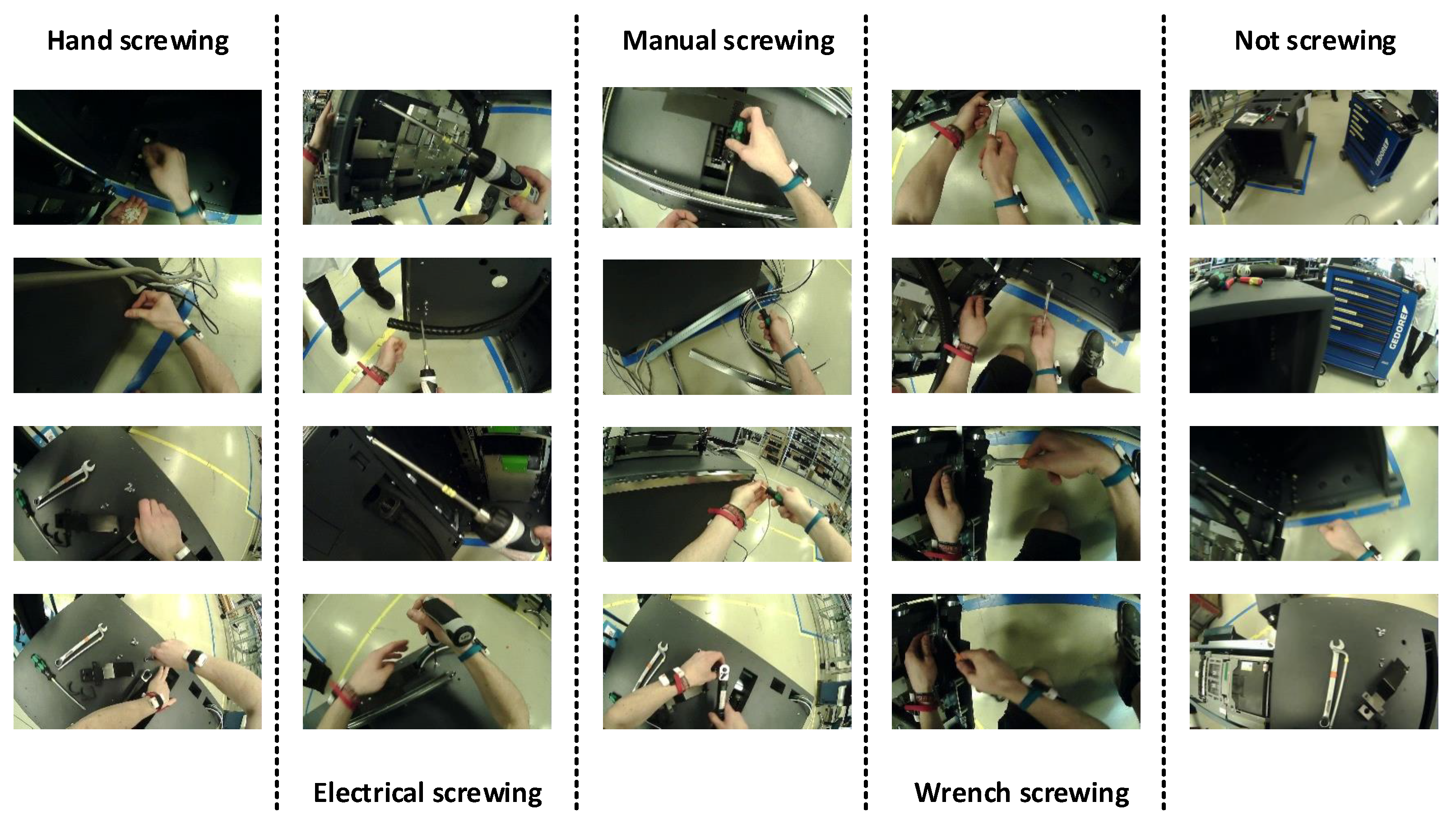
The dataset that we used in this paper was recorded at the industrial assembly lines. The scene of the assembly steps was recorded with the pupil eye tracking’s word camera. Data were recorded from the egocentric vision of the worker. The names of the classes and sample images of the classes are given in Figure 8.

Overall, 80% of the dataset was used for training the network and 20% was used to test the network’s performance. For the validation of the network, one full ATM assembly workflow was followed. The results which are shown in the results section are calculated based on the above-mentioned validated workflow.In that validation data set, there was 95% was “Not screwing” activities which were reduced to the same level as the other activities.

A total of 10 workflows were recorded, each workflow is the fully assembled ATM from scratch to the fully functional ATM. Every workflow is almost 6 h of recording. The recording of data from the RGB sensor was recorded at averagely twenty five frames per second, which was labelled with bruit force technique to separate each frame into their specified classes. All the images of the ATM assembly dataset were resized to 299 × 299. The reason for this size normalization is that the Inception-V3 was originally trained using this image size.

Prepossessing Dataset

In this step, we preprocess the dataset for the assembly action recognition before the deep neural network can be trained on the custom dataset. In literature, we have found no assembly action dataset, therefore it becomes an important part of the research to create the specific ATM assembly dataset. Assembly actions are different from the common actions (running, jumping etc.). Assembly actions are similar in our case but the tools used for screwing are different. The dataset was recorded while performing activities mostly on the main part of ATM, as can be seen in Figure 9.

The dataset of assembly actions created for this research has four different types of screwing activities. Where the tool is changed, but have the same screwing action, there are four types of screwing activities, first is screwing with an electric screwdriver, second is screwing with hand, third is screwing with a manual screwdriver and fourth is screwing with a wrench. Apart from these activities when the data were being labelled, the rest of the activities were labelled as “Not screwing”. Ten sessions of the ATM assembly have been conducted in a real industrial environment. These 10 sessions were done by 5 different workers. In the collection of the dataset, some screwing classes were dominating and some of the classes had fewer occurrences which lead to class imbalance. To manage the class imbalance problem, we undersample heavily represented classes.

Labelling was the hard part of our use case because, from hours of the videos of the recorded raw data, we had to find the micro level activities. Such a type of micro activities happens for frictions of seconds, specifically the screwing with an electrical screwdriver, which mostly lasts for one second.

Training a deep CNN requires large samples which would be sufficient to train the model, followed by the building and training of the model respectively. The network has to constantly analyze the performance to adjust the parameters of CNN with batch normalization.

To prepare the dataset for the two-stream method which was mentioned above in Section 3.2, there were two different image inputs. One was the RGB image and the second was the sequences of RGB images which were used to compile the optical flow to get the moving objects’ motions. We used the Lucas–Kanade method to create the dense optical flow of the moving objects based on the pixel intensities of an object which do not change between consecutive frames, thus the neighbouring pixels have similar motion [45].

For example, consider a pixel I (x, y, t) in the first frame. It will move by the distance of dx, dy in the next frame in time dt. If there will be no changes in the intensity, we can describe this in the Equation (1) [45].

$$I(x,y,t)=I(x+dx,y+dy,t+dt)$$

(1)

Then, the right-hand side will be the Taylor series approximation, after removing the common terms and divide with dt, thus we will receive the following Equation (2)

$$f_{x}u+f_{y}u+f_t=0$$

(2)

where

$$f_x=\frac{\partial f}{\partial x};f_y=\frac{\partial f}{\partial y}$$

$$u=\frac{dx}{dt};v=\frac{dy}{dt}$$

The equation mentioned above is called the optical flow equation, in which $f_x$ and $f_y$ are the gradients of image and same $f_t$ is the gradient along time. The Lucas–Kanade method was used to solve the u and v.

5. Results

The algorithm was implemented using Python, with 16GB RAM, dedicated 6GB Quadro GPU and Windows operating system. The networks were fully pre-trained and used for the classification task of 5 different classes which were mentioned in Section 4. We will compare the retrained model results. In the end, we will discuss the results of the model which was trained from scratch and the model which was used as a pre-trained model. Then, a 10-fold cross-validation was applied for the generalization of the classification results. Out of the total 10 recording sessions, 9 sessions were used and one session was used to check and test the model on the data set that it has never seen.

Figure 10, shows the final confusion matriceswhich were compiled. There are a lot of false positives between hand screwing and manual screwing, because the hand screwing and manual screwing are not apart from each other. If we look at the features of these two classes, there is not a big difference between the extracted features. As a result of the baseline Inception-V3, with pre-trained on the ImageNet dataset and was fine tuned on our dataset. If we look at the

Table 3. Inception-V3 model accuracy results on the five classes.

Methods	Accuracy	Weighted Accuracy	Balanced Accuracy	Precision	Recall	F1 Score
Baseline Inception V3	66.88%	73.36%	67.58%	77.02%	66.88%	68.55
Baseline Inception v3 + RNN (LSTM)	88.96%	74.12%	79.69%	82.54%	72.38%	74.35%

, the accuracy was low with the Inception-V3. The use of LSTM for the temporal information, the accuracy of the model increased significantly. Due to very low dissimilarities between the classes, it was hard for the Inception-V3 network to differentiate between the classes, but for the LSTM, that was easy because it remembers information about the previous several frame sequences.

Two-stream method’s overall training accuracy was very low, around 45%, and test accuracy was low as well. Moving cameras are a problem for optical flow algorithm because, as mentioned in Section 4 that the dense optical flow was calculated with the help of the Lucas–Kanade method, it is mainly for the moving objects, so in that case, the camera itself is moving with respect to object in the frames, so the whole frame is moved. Due to the bottleneck situation, we have decided not to further explore the two-stream method.

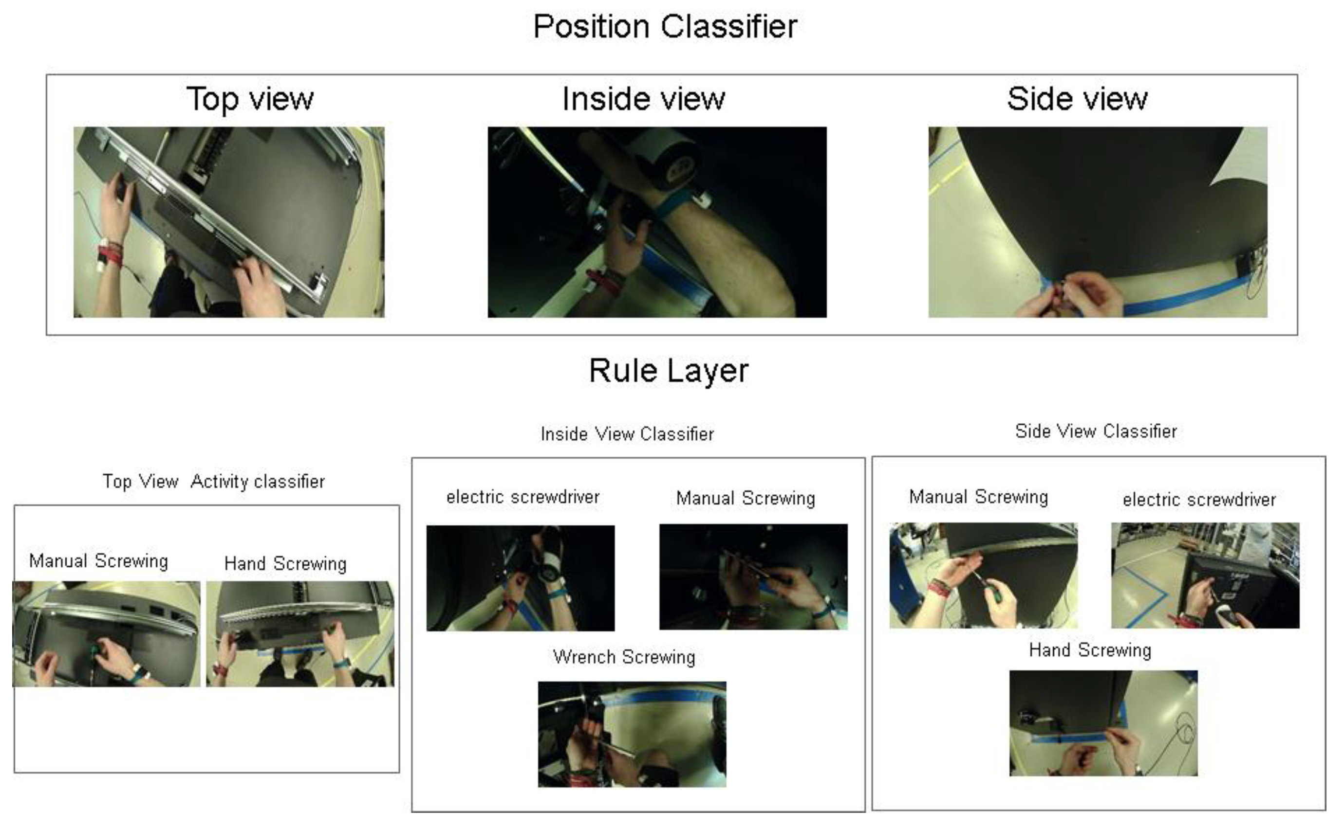
To improve the results and remove the false positives, we used four different classifiers. First, the main classifier is the position classifier, which is pre-trained Inception-V3 model, and was fine-tuned on the small dataset of different sides of the ATM where workers perform activities because, in a specific view, there are specific activities, for example, as can be seen in the Figure 11. The top view has only two types of activities, which are manual screwing and hand screwing. In the top viewing activity classifier, we just used two activities, and that is why the accuracy was 99.08%. After the first classifier, there is an if–then rule layer which provides input to the next three diffident classifiers based on the prediction of the position classifier. The results of this approach are mentioned in the

Table 4. Inception model accuracy if we divide and rearrange the dataset where the difference between classes is higher.

Methods	Accuracy	Balanced Accuracy	Precision	Recall	F1 Score
Position Classifier	95.90%	97.49%	97.94%	95.90%	96.53
Top View Activity Classifier	99.08%	99.08%	97.08%	99.08%	99.08%
Inside View Classifier	97.81%	96.19%	97.81%	97.81%	97.81%
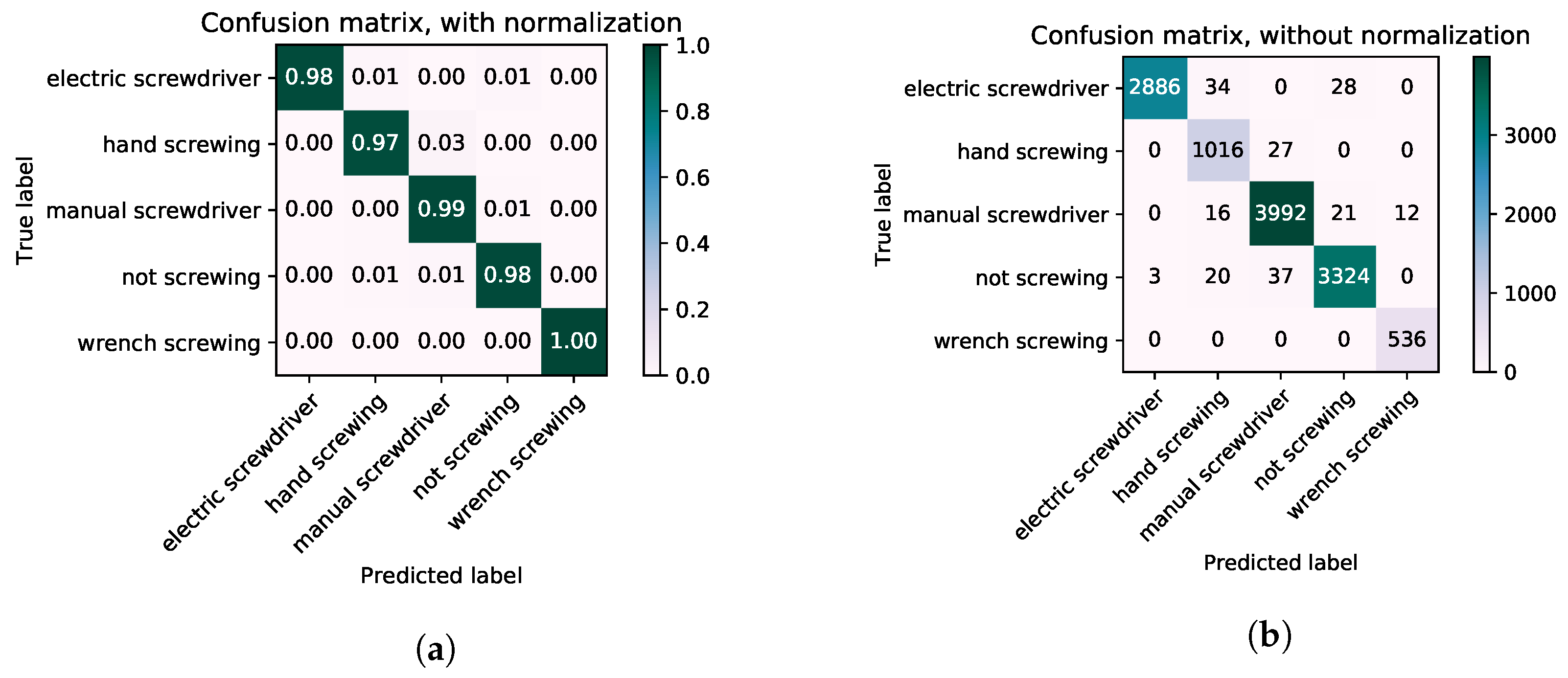
Side View Classifier	97.47%	97.60%	97.58%	97.36%	97.52%

. The classification confusion matrices can be seen in Figure 12.

We have elaborated on a table which can give the overall performance results of different networks in the

Table 5. All methods accuracy comparison.

Network Name	Accuracy	Balanced Accuracy	Precision	Recal	F1 Score
Baseline Inception v3	66.88%	67.58%	77.02%	66.88%	68.55%
Baseline Inception v3 + RNN(LSTM)	88.96%	79.69%	82.54%	72.38%	74.35%
Optimized Inception v3	78.6%	79.07%	86.90%	76.45%	80.23%
Optimized Inception v3 + RNN(LSTM)	91.40%	92.60%	96.70%	91.30%	91.10%
Baseline VGG19	74.62%	75.87%	83.89%	74.62%	76.36%
Baseline VGG19 + RNN(LSTM)	79.57%	78.75%	80.60%	77.67%	79.78%
Optimize VGG19	81.32%	84.50%	83.10%	78.93%	81.49%
Optimize VGG19 + RNN(LSTM)	83.69%	85.97%	87.65%	82.60%	83.68%

. In this table, we compared the baseline networks with optimized networks. Word baseline is used for the model which are used as a pre-trained model and was fine tuned on our classes. The optimization means the model which is trained from scratch, and all the parameters are fine tuned. Optimized and baseline networks do not have big accuracy differences. There is only one network which has crossed the 90% accuracy and that was the Inception-V3, which was trained from scratch and was combined with the LSTM network for the sequencing of the activities which have shown the results of 91.4%.

6. Discussion

The results presented in the results section demonstrate that not all assembly activities could be recognised with equal accuracy. In particular, the class of electrical screwing is often misclassified to the class not screwing. This is because there are a few of the electrical screwing activities happening before and after not screwing activities. Apart from this class, the rest of the class with features of manual tools could be recognized with a high accuracy rate. In the results obtained from the different classifiers, as mention in Table 5, the optimized Inception-V3/LSTM classifier showed the best results, as compared to baseline Inception-V3/LSTM. Where the last two layers of the Inception-V3 network was retrained and the rest of the models was pre-trained on the ImageNet dataset. In the optimized network, two blocks of the Inception-V3 have trained from scratch and the fine-tuned rest of the layers with our dataset. Training from scratch is computationally expensive but our model adapts the environment in which network performs the customised classification. The results of our model improved significantly due to the training network from scratch.

Results computed from other classifier networks were not worse in the detailed study of these results as some of the networks were performing better than Inception-V3 in some activities recognition. However, specifically recognizing the assembly activities using the tools like wrenches and screwdrivers, Inception-V3/LSTM performed best, hence we selected this network for further solution development.

To remove the false positives for the classes which were being miss classified, we have used four classifiers of Inception-V3/LSTM. As it is described in Figure 11, before classifying the activity directly, we trained the network, which will make classification based on the position of the ATM worker. This classifier is called position classifier. This approach helped to eliminate false positives.The understanding of the position is important because in a specific position, particular screwing activities are being performed. For example, in the top view, only the manual screwing and hand screwing activities are being performed. After the position classifier, there is an if–then layer which selects the classifier for the screwing activities. With this approach, we have eliminated the false positives and we obtained an accuracy level of 98.34%. The individual results of four classifiers are mentioned in Table 4 and the confusion matrices results are shown in Figure 12. The final results of the Inception-V3/LSTM classifiers with rule layers are shown in Figure 13, which clearly indicates the elimination of the false positive.

The deadset of such activities was not available publicly, hence the biggest effort was put to gather the dataset. The tools and parts which we used in our industrial use case were small, so we could not record the dataset where the camera was fixed. We decided to use the egocentric point to collect the dataset. Such a type of real environment dataset does not exist publicly. Therefore, we created the deadset from scratch. To make sure that the volume of the data is sufficient, we recorded 25 frames per second on average and one complete session was around 6 hours of recording. The labelling part was the hardest part, where we labelled the dataset using the brute force technique. We separated the micro activities which were happening for some seconds from the rest of the nonessential activities. There were lots of unnecessary activities, for example, if a worker walks towards shelves and comes back just looking at the shelves, this is not part of the workflow. Hence, we had to be careful while labelling the data. We have gone through 12 sessions of the recorded data, where we went through every single frame and separated it into relevant classes. Every step of the workflow has different micro activities, as the example showed in Figure 1. If we can achieve satisfactory results in recognition of the micro activities, then we can monitor and map these activities to macro activities. This mapping is crucial to monitor the workflow steps.

Most of the research works which are cited in the related work, they implemented deep learning networks, but implementation and results were generated on publicly available large-scale datasets. All these datasets were well organized and labelled. Some researchers have implemented deep learning techniques for industrial use cases. All these studies are using the lab-created or synthetic datasets; for example, in [8], the author implemented the 3D-CNN network for the monitoring of industrial process and steps. This dataset was created in a controlled environment. They planned work steps and different participants repeated the same actions in the same sequences. Results from this study are promising but these networks are performing in a lab environment, not in the real-world environment. Authors in these studies [9,10] used the TCN and two-stream networks for the action classification respectively. The datasets used in these studies are UCF101 [19] and HMDB51 [46]. UCF101 is the dataset about the sports activities and HMDB51 is video dataset, consists of human actions like smile, laugh, clapping and brushing hair etc. Methods used in these two studies are performing well on these datasets, but these methods face problems when they are applied in a real-world environment. In our case, we have implemented the two-stream method and the accuracy was around 45%. In our case, the moving camera creates a bottleneck situation that creates a problem in the accurate calculation of optical flow, which leads to inaccurate predictions. Researchers in [47] provided a method which could map the wood assembly products and can control any discrepancies, but the experiments that they presented are not in the real-world environment. In [23], the author used many different publicly available datasets, where the author used PSPNet which is based on classifying every single pixel in the scene and then making a relation out of these pixels. This is a computationally expansive method which shows promising results. The author of this study used the PASCAL VOC [48] dataset to implement and compute the results.

In our work, we have implemented these networks in a real-world industrial use case where workers are free to do what they usually do. We did not have any control over the worker’s working style. We have proposed a pipeline on how to implement state of the art deep learning networks in a real-world industrial environment, to monitor the industrial assembly process. Our proposed method can be reused in all industrial assembly processes where the assembly sequence is substantial and the assembled components are small. To achieve high accuracy, we must identify micro activities in those industrial processes. If micro activities can be recognized with satisfactory accuracy, these micro activities can be associated with work steps at the macro level.

In our proposed approach, there are weaknesses which need to be addressed in the future. The main weakness is that our approach does not work properly in bad lighting conditions. As the lighting goes bad, the accuracy was dropped; this is due to the bottleneck condition. Our model is trained on the bright scene images. In future, to deal with this problem, we will introduce diffident data streams, for example wrist-worn, accelerometer sensors, or the microphone which could help the model to recognise the activities in bad lightning strikes.

7. Conclusions

In this research, we proposed a model to control the assembly process of an ATM. Existing deep learning models to control the assembly process have been implemented on publicly available datasets. These datasets are either synthetic or generated in controlled environments. The dataset for this study was collected in an uncontrolled real-world environment. We implemented four different models to recognise the micro activities in the assembly process. The monitoring and recognition of micro activities in the ATM assembly process are complicated due to the tiny nature of components and uncontrolled working style of workers. Due to the nature of the data, we made modifications in existing deep learning models to fit for the task. The classification was challenging, having classes with very minor differences among them. The problem of the false positive was tackled with the addition of the rule layer between different classifiers. This modification improved the accuracy level from 91.40% to 98.34%. The results show that the assembly line sequence could be controlled using deep learning models. Our proposed model with the Inception-V3/LSTM will generate feedback in case of any discrepancy in micro activities by the worker. The core contributions of this paper are the recognition of micro activities during the assembly process in a real-world environment, the proposed modified deep learning model for the assembly process and normalization of the uncontrolled environment data.

The proposed model is suitable for all those assembly processes which involve tiny components. Tools should be visible during the screwing of components. However, if there are assembly processes where tools are partially occluded, then this model will have limitations. As future work, we will use sensors to deal with this occlusion problem. We will also use an eye-tracking dataset because with the help of the eye-tracking dataset, we can localize the region of interest in a single frame which could make the model more efficient.