Abstract
The growing demand for hydrocarbons has driven the exploration of riskier prospects in depths, pressures, and temperatures. Substantial volumes of hydrocarbons lie within deep formations, classified as high pressure, high temperature (HPHT) zone. This study aims to delineate hydrocarbon potential in the HPHT zone of the Malay Basin through the integrated application of rock physics analysis, pre-stack seismic inversion, and artificial neural network (ANN). The zones of interest lie within Sepat Field, located offshore Peninsular Malaysia, focusing on the HPHT area in Group H. The rock physics technique involves the cross-plotting of rock properties, which helps to differentiate the lithology of sand and shale and discriminates the fluid into water and hydrocarbon. The P-impedance, S-impedance, Vp/Vs ratio, density, scaled inverse quality factor of P (SQp), and scaled inverse quality factor of S (SQs) volumes are generated from pre-stack seismic inversion of 3D seismic data. The obtained volumes demonstrate spatial variations of values within the zone of interest, indicating hydrocarbon accumulation. Furthermore, the ANN model is successfully trained, tested, and validated using 3D elastic properties as input, to predict porosity volume. Finally, the trained neural network is applied to the entire reservoir volume to attain a 3D porosity model. The results reveal that rock physics study, pre-stack seismic inversion, and ANN approach helps to recognize reservoir rock and fluids in the HPHT zone.
1. Introduction
Reservoir characterisation is a process that combines all the available field data from various data sources to characterise different reservoir properties in spatial variability quantitatively [1]. These properties play a significant role in petroleum field operations and reservoir management [2,3]. The main data sources include seismic, well logs, and core data. Integrating these data sources improves the reservoir characterisation process and reduces uncertainties [4,5]. Moreover, integrating various techniques showed effectiveness in reservoir characterisation. Such approaches tend to reduce uncertainties and enhance reservoir properties’ prediction [6,7].
The exploration of high-pressure and high-temperature (HPHT) fields is a current leading-edge in oil and gas commerce. The expanding need for hydrocarbons around the globe has driven the search for new resources in the exploration and production industry. The new resources are mostly located in deeper formations as earlier explorations regularly focused on shallower formations. Drilling into deeper formations may result in encountering higher pressure and temperature zones. HPHT fields have widely occurred in the Gulf of Mexico, the North Sea, Southeast Asia, Africa, and the Middle East. Research has projected that from over 100,000 wells drilled worldwide in 2012, almost 1.5% of the wells can be classified as HPHT [8]. These wells are frequently discovered in regions where the exploration of new horizons is in progress. Although the number is relatively small, the wells usually indicate important potential resources. According to the American Petroleum Institute (API), a well is defined as HPHT when it encountered pressure more than 15,000 psi (103 MPa) and the temperature exceeds 350° F (177 °C) [8].
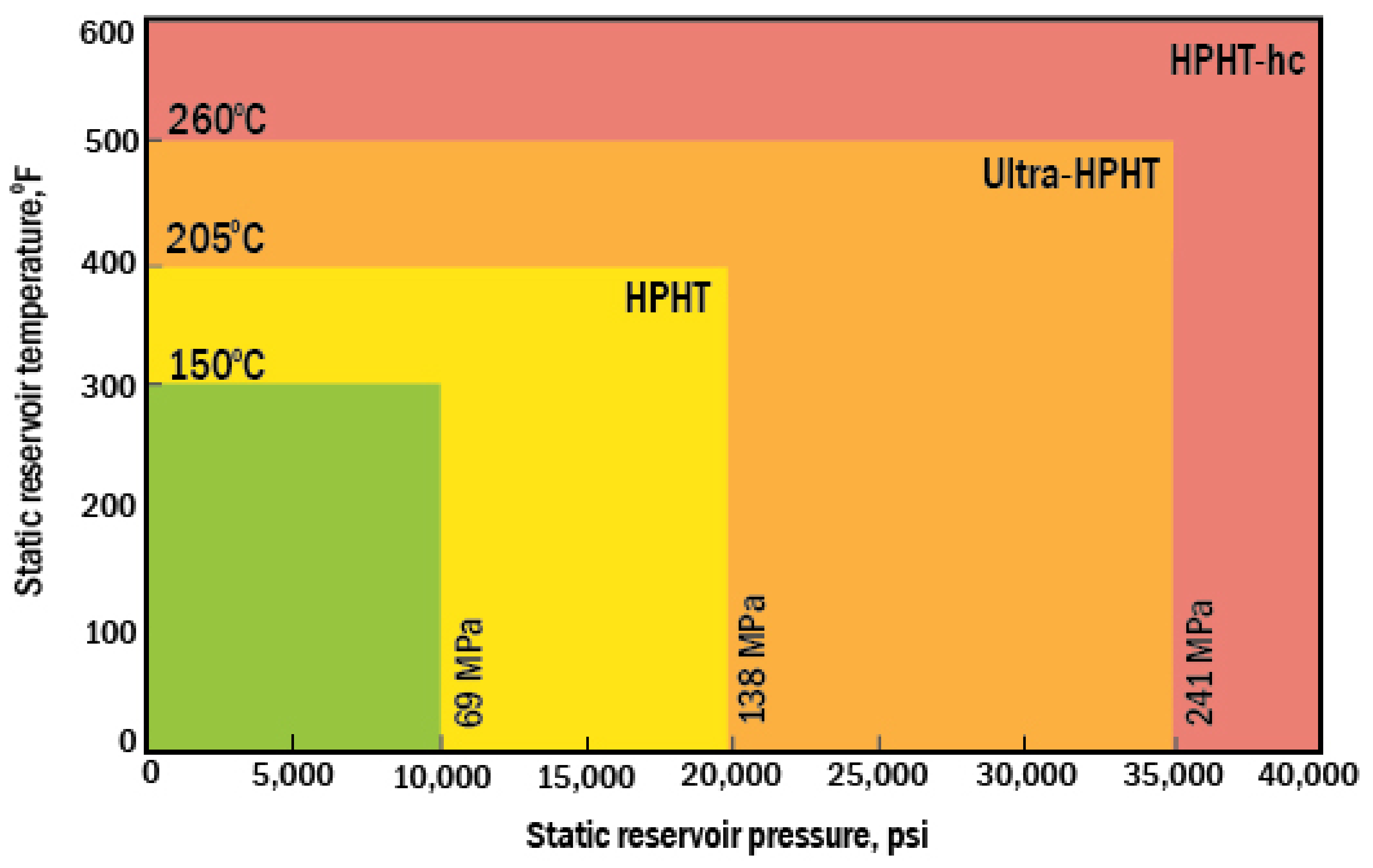
Figure 1 demonstrates an in-depth classification of HPHT specifications by Schlumberger. The classification is based on a structure that considers the thermal stability of design components, appropriate electronics, and pressure ratings of hardware. Based on this classification, the HPHT operations are segmented into three main tiers. Tier I refers to the HPHT zone for the wells with reservoir pressure within 10,000 psi to 20,000 psi and reservoir temperature between 300° F to 400° F. Tier II is defined as ultra HPHT, which involves any reservoir with pressure exceeding 20,000 psi and less than 35,000 psi and temperature amidst 400° F to 500° F. Tier III involves extreme HPHT wells, with reservoir pressure ranges from 35,000 psi to 40,000 psi and temperature within 500°F to 600° F. The HPHT-hc is categorised according to situations that rarely occurred in oil and gas wells, even though geothermal wells may surpass 500° F and several deep-water wells have downhole pressure that exceeded 35,000 psi [8].

Figure 1.
HPHT classification by Schlumberger [8].
HPHT conditions influence each phase of production and development, which involves the drilling risers, sensors, safety control valves, and blowout preventer (BOP) control systems. Due to high-pressure conditions during completions, testing, and production operations, a possibility of hazard to personnel working with equipment may occur. To administer the exposure to hazard and permit safe wellsite operations, the engineers work with appliances solely constructed to operate above the predicted maximum pressure. Before using equipment, they are assessed above the highest predicted pressure to ensure operations can be performed safely [9].
This research focuses on identifying the hydrocarbon potential of the HPHT zone of the Sepat field, located in Malay Basin using seismic and well log data by applying rock physics study, simultaneous seismic inversion, and ANN.
The rock physics study mainly involves cross-plotting of several rock properties. Cross-plots are a visual description of the connection among two or more parameters that enable simultaneous and meaningful evaluation of two attributes with ease. Typically, the cross plots are used to visibly recognise or observe anomalies, which could be inferred as the existence of hydrocarbons or other fluids and the type of lithology. Cross-plotting appropriate rock properties allow straightforward interpretation by clustering the cross-plotted data’s common lithologies and fluid types.
Pre-stack simultaneous inversion is a seismic exploration method frequently used to identify oil and gas and characterise lithology. Simultaneous seismic inversion involves the invert of seismic reflectivity into elastic rock properties to evaluate the properties of the reservoir away from the well. Many studies and practices have demonstrated that pre-stack simultaneous inversion may accurately forecast gas-bearing reservoirs. The trick is to select a reasonable approximation of the Zoeppritz equation as the basis for the inversion [10]. The original reflectivity data are converted from an interface property (reflection) to an elastic rock property [11]. Using seismic inversion, the effect of wavelet can be reduced as inversion replaces seismic blocks of impedance at a particular time sampling interval. This study utilises pre-stack seismic inversion, whereby seismic angle or offset data are transformed into P-Impedance (Zp), S-Impedance (Zs), Vp/Vs ratio, and density volumes through the incorporation of seismic angle/offset gathers, well data, and a basic stratigraphic interpretation.
ANNs have been successfully applied in reservoir characterisation [12]. The major objective of ANN application is to integrate acquired data from various geological, petrophysical, geophysical sources in reservoir characterisation by identifying the complex non-linear correlation of this input data [5].
2. Geological Background
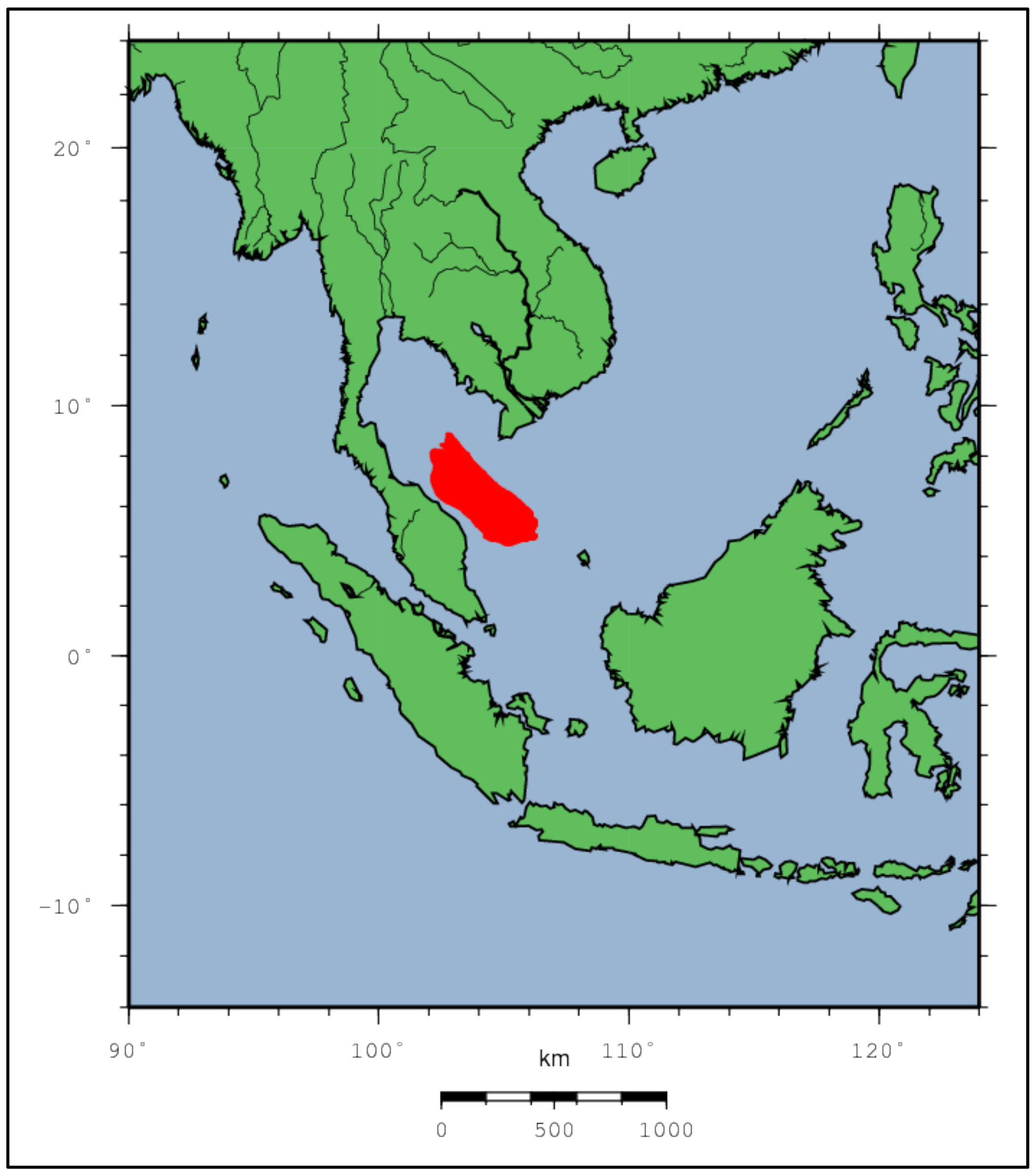
The study of the HPHT zone is conducted using the data from Sepat Field located in Malay Basin (Figure 2). Malay Basin had experienced three major structure movements, involving extension, thermal subsidence, and basin inversion (Figure 3). This basin originated by extension during Late Eocene to the Early Oligocene and subsequently by thermal subsidence during Miocene to recent [13]. Sedimentation during Miocene was accompanied by structural inversion that caused the growth of major east-trending anticlines in the axial part of the basin. Exploration activities in the Malay Basin had started in the late 1960s, which resulted in discoveries of several fields. Most of the explorations targeted the conventional play type in Upper Miocene clastic of Group D, E, and Top F. The play in these groups is commonly situated within the hydrostatic to slightly overpressured zone; usually at the upper region of the pressure ramp up. Depositional environment for Group A, B, and D is interpreted as fluvial and delta front progradation sand, Group E as lower coastal plain, Group F as delta front to shallow marine. According to Uttarathiyang and Piggott, the sediments of Group H are described to be marine deltaic owing to their general correlation to the global sea-level curve [14]. The hydrocarbon accumulations in this basin are mostly trapped within the east to west faulted anticlines in Group E, characterised by siliciclasticprone. The previously discovered hydrocarbon forms are generally gas with condensates, and some oil rims have been observed.
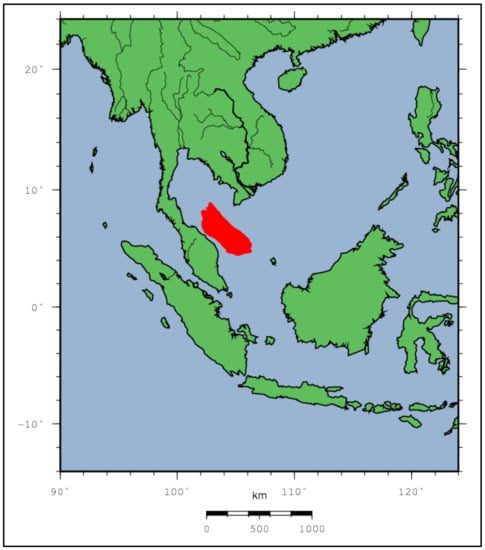
Figure 2.
Geographical map of Malay Basin.
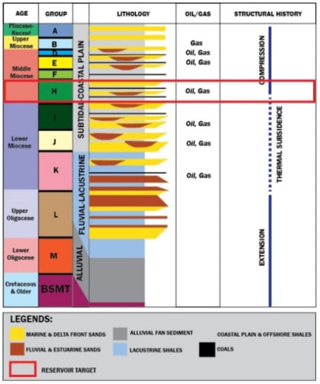
Figure 3.
Regional stratigraphic column of the Malay Basin and the reservoir target which is highlighted by a red rectangle. The study is focused on a reservoir target in Group H (modified from [13]).
Sepat field is located in Block PM313, approximately 180 km northeast of Kertih, Terengganu, and 80 km northwest of the Dulang Field, with an approximate area of 30 km by 12 km. The structure of the Sepat field is an east-west elongated anticline. Two major normal faults bound the field in the eastern and the western boundary. In the central area, this field is intersected by several northeast-southwest trending normal faults that may cause compartmentalisation. The Sepat structure dips gently to the west before rising again across a saddle to form the West Sepat structure. Seismic data in the Sepat Field is poorer in deeper depths and affected by gas clouds from the shallower reservoirs. The reservoirs consist of the fluvial and coastal plain sand, while the traps are associated with four-way dips anticline. HPHT play in the Sepat Field begins from the Middle to Lower Miocene of Group F, H, I, and J, categorised by the simultaneous event of HPHT. The reservoir pressure system is over pressured starting from a depth of 1780 m. As the earlier exploration encountered a constraint to drill through the HPHT region, most of the drilled wells had only penetrated until the top of Group F. This study will emphasise the HPHT region in Group H of Sepat Field (Figure 3).
3. Dataset and Methods
3.1. Dataset
3.1.1. Well Data
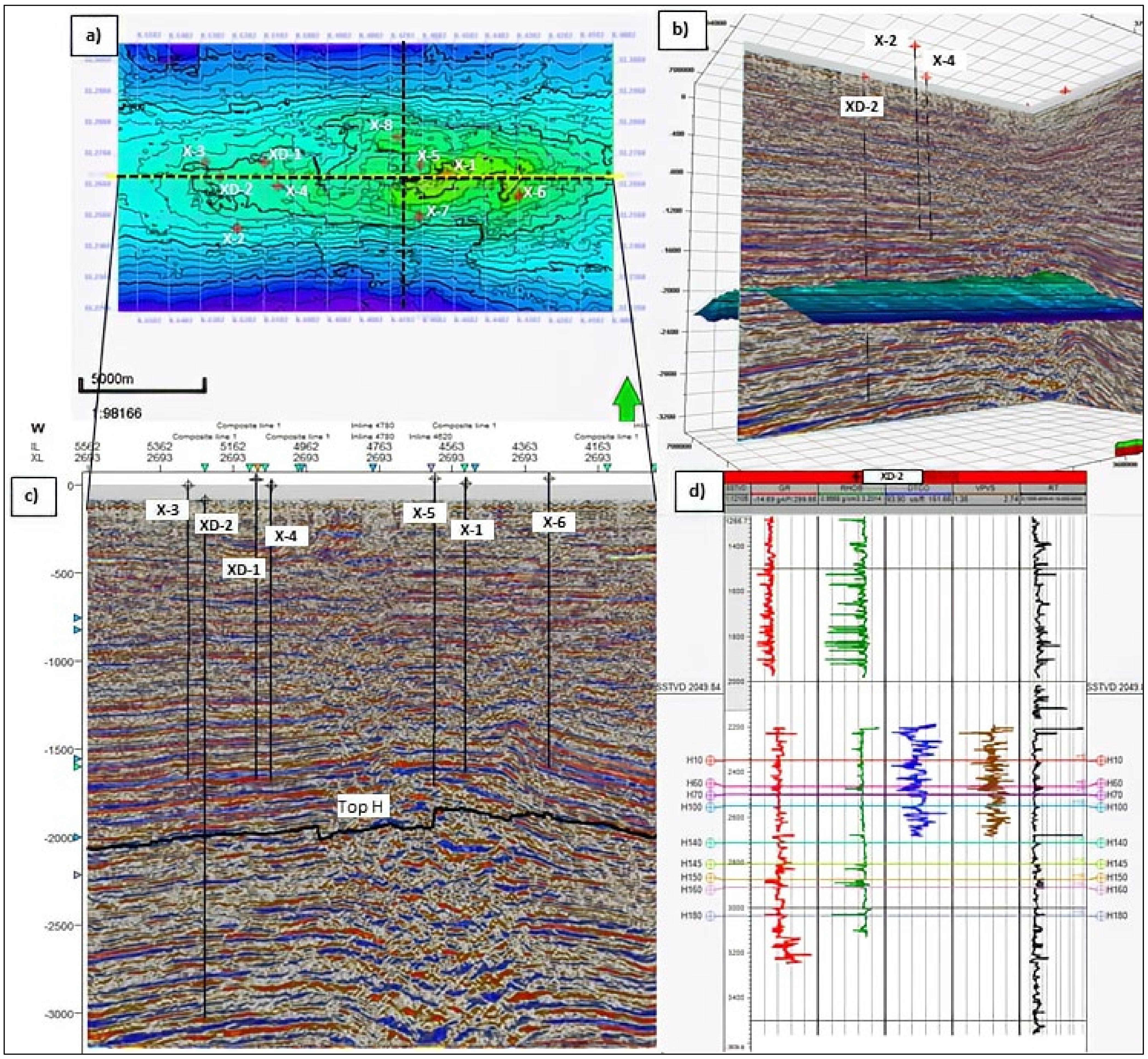
The available well log includes datasets from ten wells, i.e., XD-1, XD-2, X-1, X-2, X-3, X-4, X-5, X-6, X-7, and X-8. The available well log consists of gamma-ray, neutron porosity, density, resistivity, compressional wave velocity, and shear wave velocity logs. However, only XD-2 well contains the information obtained from the HPHT zone. The data from other wells was used for ANN testing and validation purposes. After loading and checking of log data, it was identified that log editing and conditioning were required (Figure 4d). The well log conditioning involved processes of de-spiking and filling the gaps. Therefore, the data of low quality was recognised and substituted by synthesised data [15].
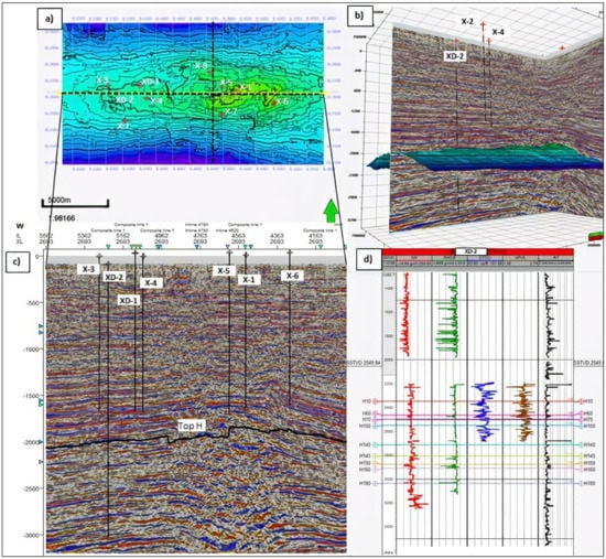
Figure 4.
(a) Map of seismic geometry with well locations; (b) Interpreted horizon Top H and well locations; (c) Migrated seismic section view; (d) Logging profile of XD-2 well.
3.1.2. Seismic Data
The 3D seismic dataset consists of pre-stack near (5–15 degree), middle (15–25 degree), and far (25–40 degree) migrated angle stacks. The 3D seismic dataset was acquired and processed in 2002 and covered a 266 km2. The record length of data is 5 s. The quality of seismic data ranges from good to fair. Most of the reflectors are not continuous in the deeper section. They are poorer in resolution due to the effects of gas clouds from the shallower reservoir. A summary of seismic processing flow is:
- Navigation merge;
- Designature;
- Geometrical spreading amplitude compensation;
- Swell noise attenuation;
- Q compensation;
- Predictive deconvolution;
- Radon demultiplex;
- 3D interpolation and regularisation;
- Velocity analysis;
- Pre-stack time migration;
- Sort to angle gathers.
The parameters above were applied to optimize the image of the seismic section up to the zone of interest, which is the H Group. The left-over multiples in the deeper section did not affect our results.
Figure 4a,c demonstrate the map of seismic geometry with well locations and migrated seismic section view, respectively.
3.2. Methods
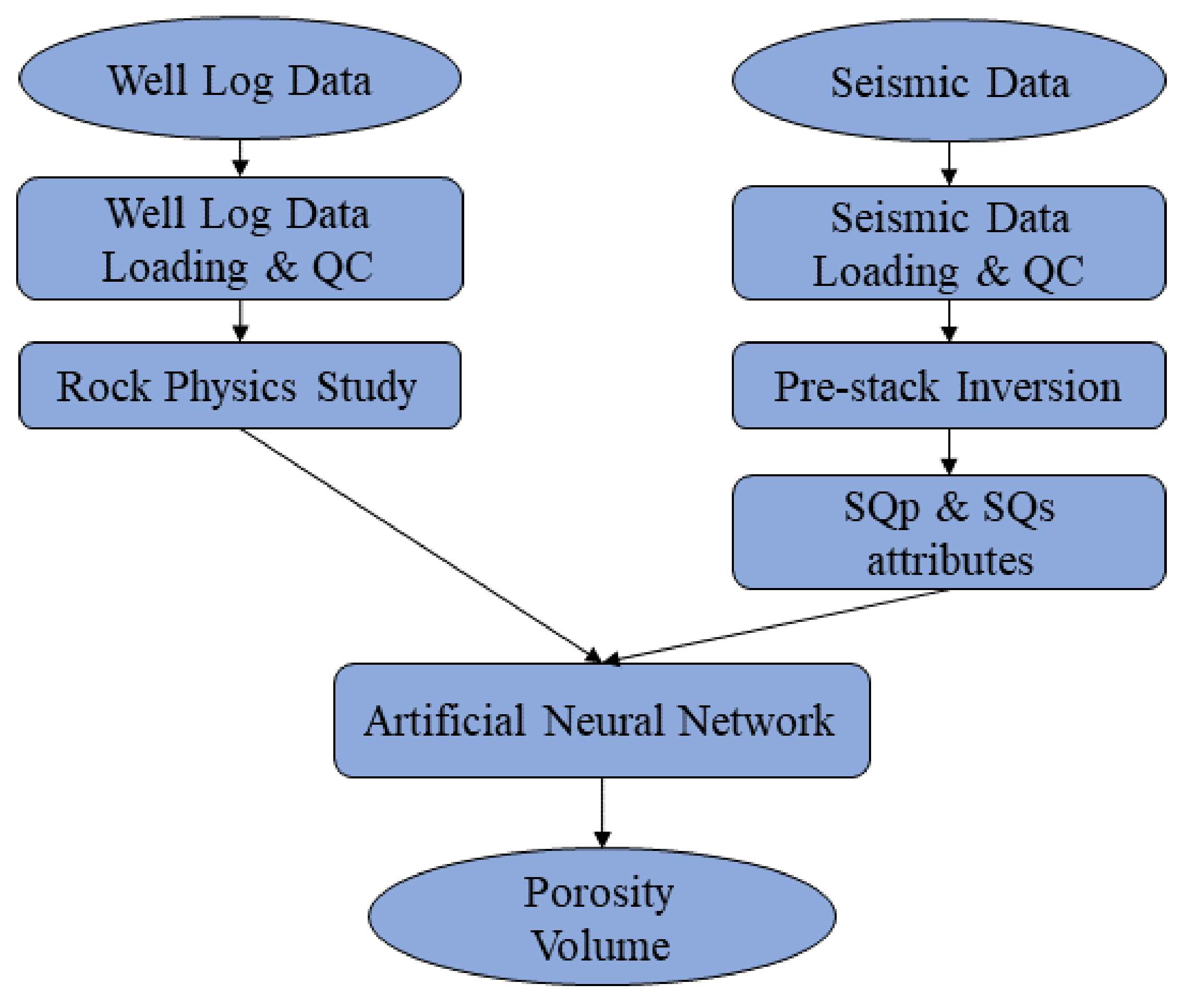
This research paper is focused on (1) rock physics study, (2) the acquisition of 3D elastic properties using simultaneous inversion, (3) the generation and analysis of SQp and SQs volume attributes, (4) the application of ANN to evaluate porosity of the study field. Figure 5 demonstrates the proposed workflow for reservoir characterisation to reduce reservoir modeling uncertainties of the HPHT zone of the Sepat Field.
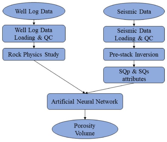
Figure 5.
The workflow for reservoir characterization of HPHT zone in Malay Basin.
3.2.1. Rock Physics Study
The cross-plotting approach was used in rock physics study. The main aim of this approach is to visibly recognise or observe anomalies, which could be inferred as the existence of hydrocarbons or other fluids, and the type of lithology. Three types of cross-plots are generated in this study, i.e., Vp/Vs ratio versus P-Impedance, SQp versus SQs, and lambda-rho versus mu-rho. The cross-plot zonation is then carried out to identify the cluster patterns of lithology and fluid type from the resulting elastic parameter cross-plots.
A direct understanding of the reservoir characterisation can be obtained from Lamé parameters, which normally consist of lambda (λ) and mu (μ) parameters. A cross-plot of lambda-rho (λρ) versus mu-rho (μρ) can be used to classify the lithology and types of pore-filled fluids. λρ and μρ are derived from P- and S-Impedances, as in Equations (1) and (2). The basic principle in characterising lithology from the perspective of the Lamé parameter is the relationship amidst incompressibility (λ) and rigidity (μ) [16]. An implication of grains organisation can be gained through the dispersion of stress between Lamé parameters when a rock experiences effective stress. For instance, when a substance is more incompressible than rigid (λ > μ), an anisotropic division of stresses distorts the grain shape, causing considerable aspect ratios. These types of grain shapes are frequently discovered in laminated shales. Suppose there is equal dissemination of stress (λ = μ). In that case, the grains are identified as having an aspect ratio of 1, or the grains are randomly ordered. This grain characteristic is regularly observed in the sand. Therefore, the ratio of lambda to mu is beneficial in recognising shale versus sand lithologies [17]. For fluid identification, considering the rock characteristics do not alter, the Lamé parameter affected is only λ. As an example, sand can be filled with various types of fluids. The fluid will reduce the incompressibility of the sand. The incompressibility is least affected by brine, while gas is affected the most. The following are the Equations (1) and (2).
where 2.0 ≤ c ≤ 2.5, ρ represents density, Zp is acoustic impedance, Zs is shear impedance [16].
Furthermore, the novel attributes, SQp, and SQs attributes were implemented in rock physics study in this work. These attributes allow minimising the ambiguity in reservoir characterisation from seismic data. The SQp and SQs attributes were also implemented to enhance petrophysical properties prediction accuracy. These attributes were derived from elastic properties and successfully proved their effectiveness in formation evaluation, reservoir characterisation, facies classification [18,19,20]. SQp attributes have a similar response as gamma-ray that indicate the lithology.
In contrast, the SQs attribute gives a similar response to resistivity. SQp and SQs attribute in well log scale has been successfully patented [21]. SQp and SQs attributes were derived from the following equations:
where M/G is the bulk and shear modulus ratio that can be approximated from the P-wave and S-wave velocity ratios [22]. Equations (3) and (4) were implemented on well log data to produce the SQp and SQs logs.
Furthermore, the 3D SQp and SQs attributes were generated from basic elastic properties, density, Vp, and Vs obtained from the seismic inversion process.
3.2.2. Pre-Stack Inversion
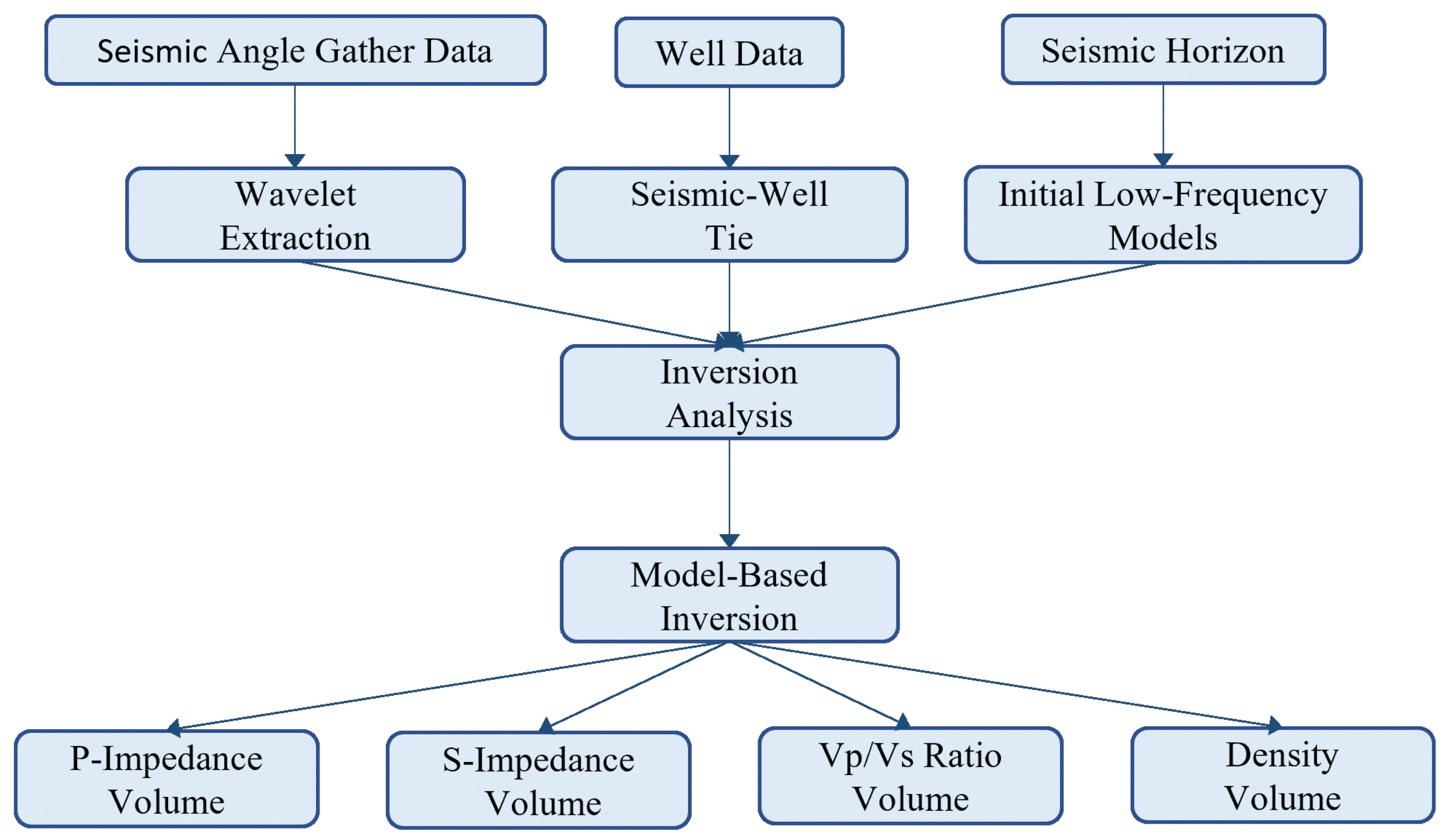
Simultaneous model-based inversion was performed to obtain density, P-impedance, S-impedance, and Vp/Vs ratio volumes from the available pre-stack seismic data. Furthermore, these outputs were utilized to acquire 3D models of SQp and SQs attributes and serve as input for ANN modelling. The workflow of the pre-stack inversion process is shown in Figure 6. A detailed description of each step of the pre-stack inversion process is discussed further.
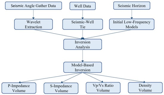
Figure 6.
The workflow of the pre-stack inversion process.
The main input data for pre-stack inversion consists of 3D pre-stack seismic (near-, mid-, far-angle) volumes, well data and a set of horizons to guide the interpolation of the initial model. The pre-stack inversion in this study was conducted using data from XD-2 well, which penetrated the zone of interest, the HPHT zone.
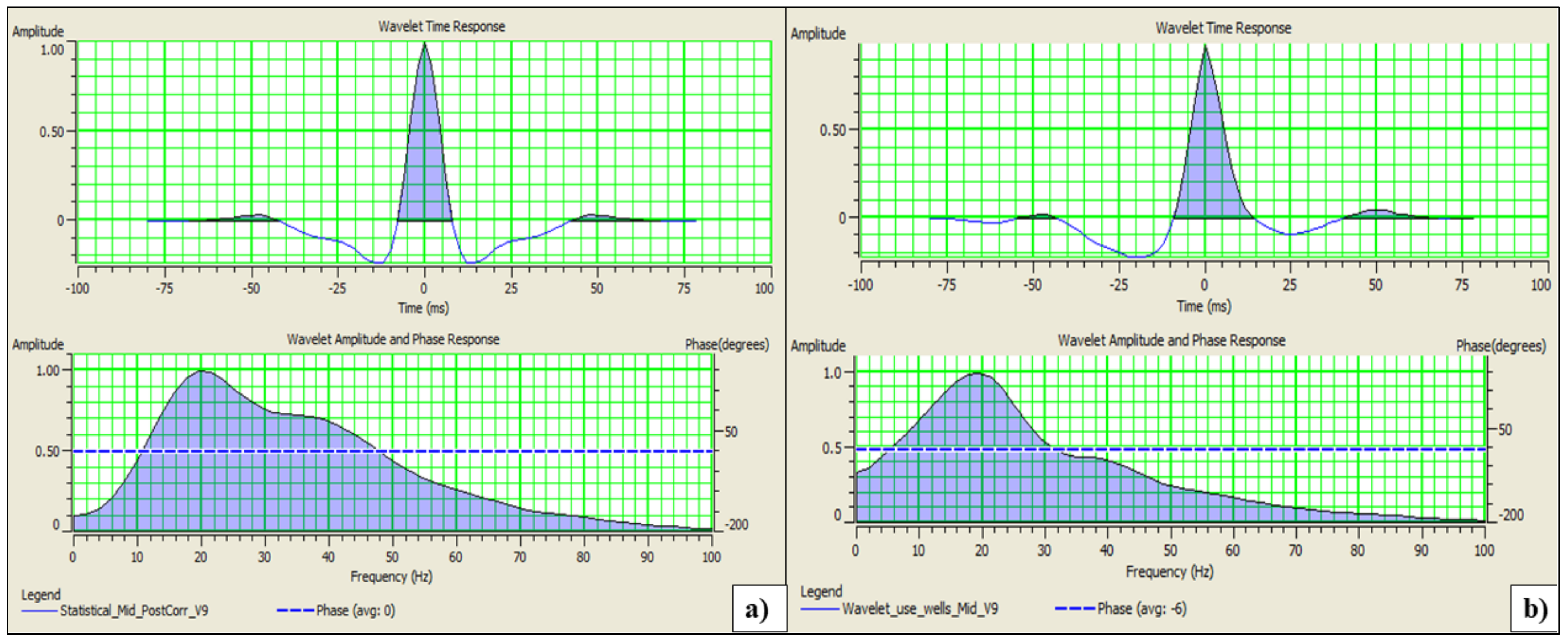
The inversion process involves seismic-well tie, low-frequency model generation, and model-based inversion [23,24,25]. Three groups of wavelets-angle-dependent are extracted from the near, middle, and far angle gathers (examples in Figure 7). An angle-dependent wavelet is extracted for each gathers group for near (5° to 15°), middle (15° to 25°), and far (25° to 40° gathers), respectively. For seismic-well tie, the determined wavelet is convolved with the reflectivity of well XD-2.
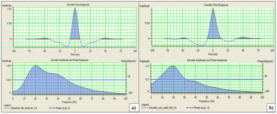
Figure 7.
(a) The extracted statistical seismic wavelet and (b) The extracted wavelet from wells.
The initial low-frequency models of P-wave, S-wave, Vp/Vs ratio, and density are built on interpreted seismic horizons and corrected sonic and density logs. The values from well log data are extrapolated using the trend from the logs and the interpolation guided by the interpreted 3D horizons. These models were then used as the input for the inversion process.
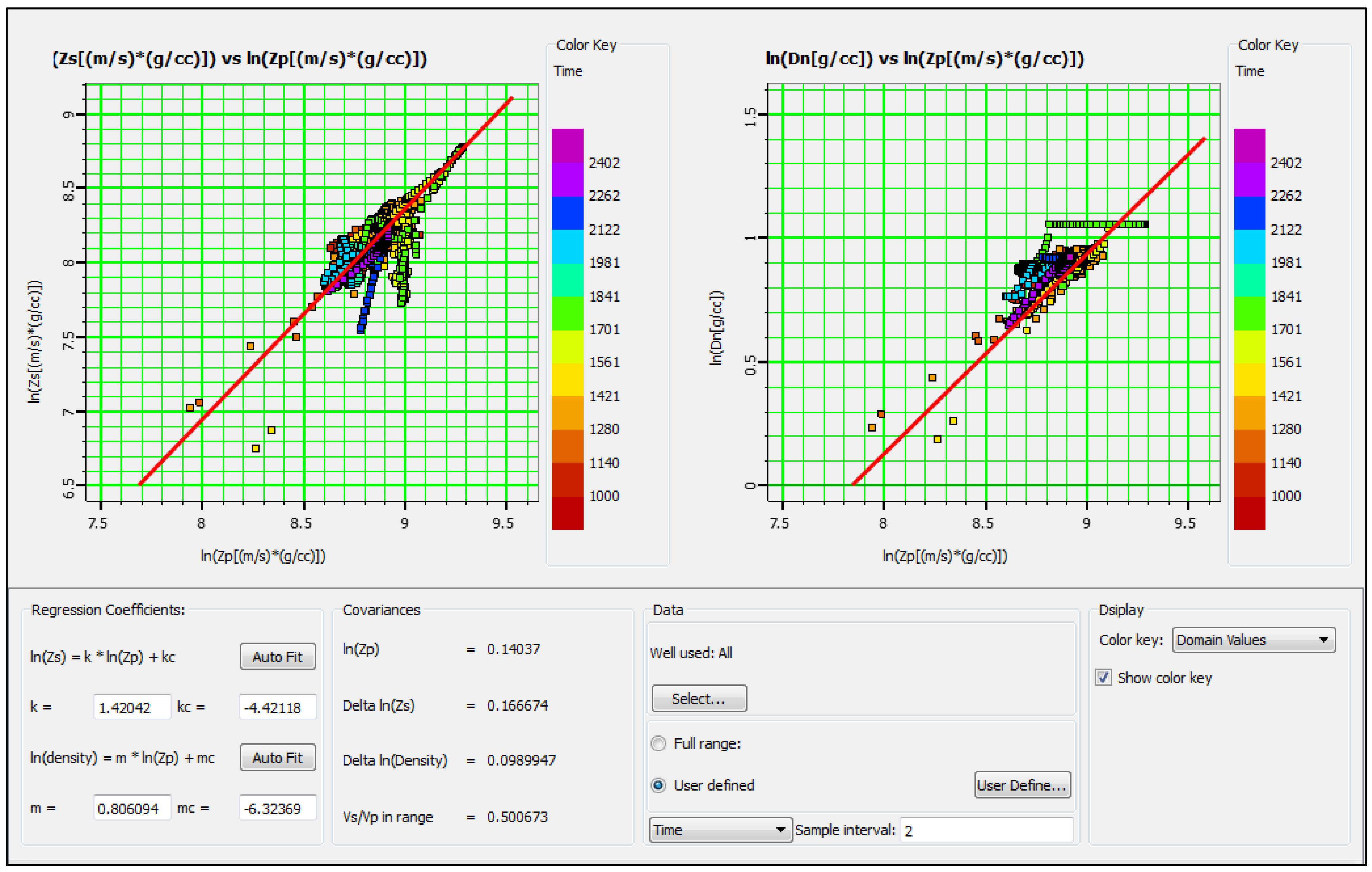
An inversion analysis is conducted on the inverted seismic models at the location of the XD-2 well to obtain optimum inversion parameters before seismic volume inversion. The important inversion parameters, such as regression coefficient, background ratio of Vp/Vs, pre-whitening, and muted dead traces are optimised to minimise the root mean square (RMS) error values calculated from inverted Zp, Zs, and density to the respective original logs. The optimised regression coefficient is determined by cross-plotting the inverted logarithmic Zs versus inverted logarithmic Zp and inverted logarithmic density versus inverted logarithmic Zp and location, as shown in Figure 8. After all, parameters are determined, the inversion result is analysed by evaluating the error and correlation of the inverted Zp, Zs, and density. Only inversion parameters with the lowest error and highest correlation values are selected and applied in the final seismic volume inversion for quality control.
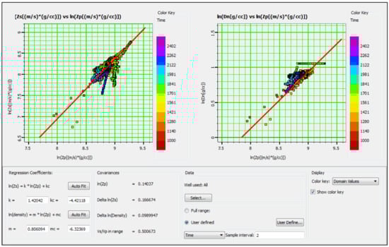
Figure 8.
Regression coefficients, as determined from elastic rock property cross plot. The outputs of simultaneous inversion of P-impedance, S-impedance, density, and Vp/Vs ratio were further implemented to generate 3D cubes of SQp and SQs attributes. Additionally, these outputs were also used for further ANN modelling.
3.2.3. SQp and SQs Attributes
The outcomes of pre-stack simultaneous inversion, Vp/Vs, and density 3D cubes are implemented to generate 3D SQp, and SQs attributes through math trace and equation. Equation (3) was used to generate 3D SQp attributes, and Equation (4) was utilized to obtain 3D of SQs attribute.
These attributes are proven to be effective in litho-fluid delineation [26]. The changes of these attributes’ values will help to identify hydrocarbon-bearing intervals and their continuity in sections. Low values of SQp attribute indicate the presence of sand lithology and high values of SQs attribute indicate the sand porosity filled with hydrocarbons [27]. The sections and averaged data horizons of SQp and SQs attributes were analyzed to identify hydrocarbon-bearing zones and their continuity.
3.2.4. Artificial Neural Network (ANN)
Radial basis function network (RBFN) technique is implemented using seismic and well data to map porosity of HPHT zone in the Sepat Field.
The RBFN technique was first introduced by Powell in 1987 [28] and first applied by Schultz et al. in 1994 [29]. Several works have shown the effectiveness of the RBFN technique in reservoir characterisation [30,31].
RBFN is a feed-forward neural network where the Gaussian bell curve is the basis function. In RBF, each training point has a weight, and the weights are multiplied by Gaussian functions of the attribute distances. A sigma parameter controls these Gaussian functions. The fitting function is . Note that g is used instead of φ in some publications. The non-linear functions jj are called “basis” functions.
Mathematically, the basis function is:
where, and σ is the sigma parameter, a smoothing parameter. is the scaled distance between the point we are estimating, xn and the training point, sj. The smoothing parameter does the scaling. The computation of the predicted values can be written as:
N = 1,2…
M and xn are unknown. M is the number of unknown values. RBFN develops a spatial relationship between the seismic attributes and the training data and works in M-dimensional space. The weights are pre-computed using a generalised matrix inversion of the basis functions weighted by the training values.
4. Field Application and Results
4.1. Rock Physics Study
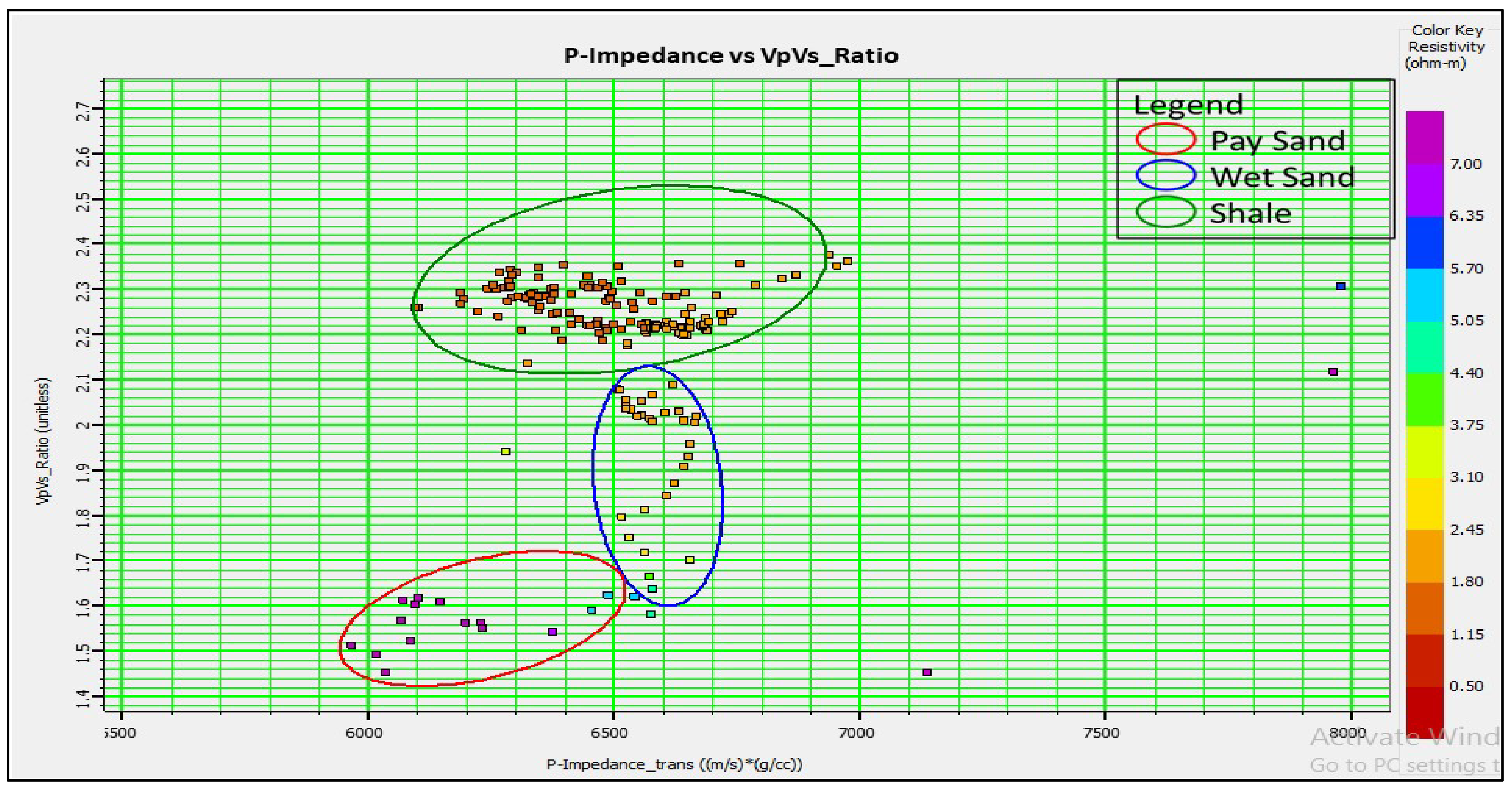
Lithological and fluid characterisation of the HPHT zone is performed at the location of XD-2 well by cross-plotting analysis. It comprises of Vp/Vs versus Zp, μρ versus λρ, and SQp versus SQs. The data between Top H and H60 are used in the cross plots by scrutinising the trend of the two rock physics elements plotted on the x- and y-axis. In most cases, the rock physics template consisting of Vp/Vs versus Zp shows a diagonal separation of fluid and lithology diagnostic zones on the cross plots. Such characterised diagonal zones are due to the low Vp/Vs and Zp of the hydrocarbon-filled zone, increasing Vp/Vs and Zp values with fluid change from hydrocarbon to the water-filled zone. Vp/Vs is a good fluid indicator as Vp has a higher sensitivity to fluid changes, whereas Vs is not, except in the special case of very viscous oil. The Vp/Vs versus Zp cross-plot results in Figure 9 showed three distinctive zone separations, with the lowest Vp/Vs and Zp zone outlined in red identified as the pay zone. The characterised pay also showed the highest measured resistivity around 8 Ωm in purple-coloured data indicating the presence of hydrocarbons. The medium Vp/Vs and Zp values outlined in blue are characterised as wet sand. The measured resistivity ranges from 1.8 Ωm to 3 Ωm. The highest Vp/Vs and Zp values in the green outline represented the shale lithology, with the lowest resistivity value zone. The characterised zone of Vp/Vs versus Zp cross-plot data based on the measured resistivity provided a good insight into the HPHT reservoir characterisation obtained from the inversion results.
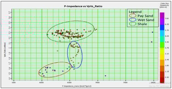
Figure 9.
Vp/Vs ratio vs. P-impedance cross plot with colour-coding based on resistivity for pay sand delineation.
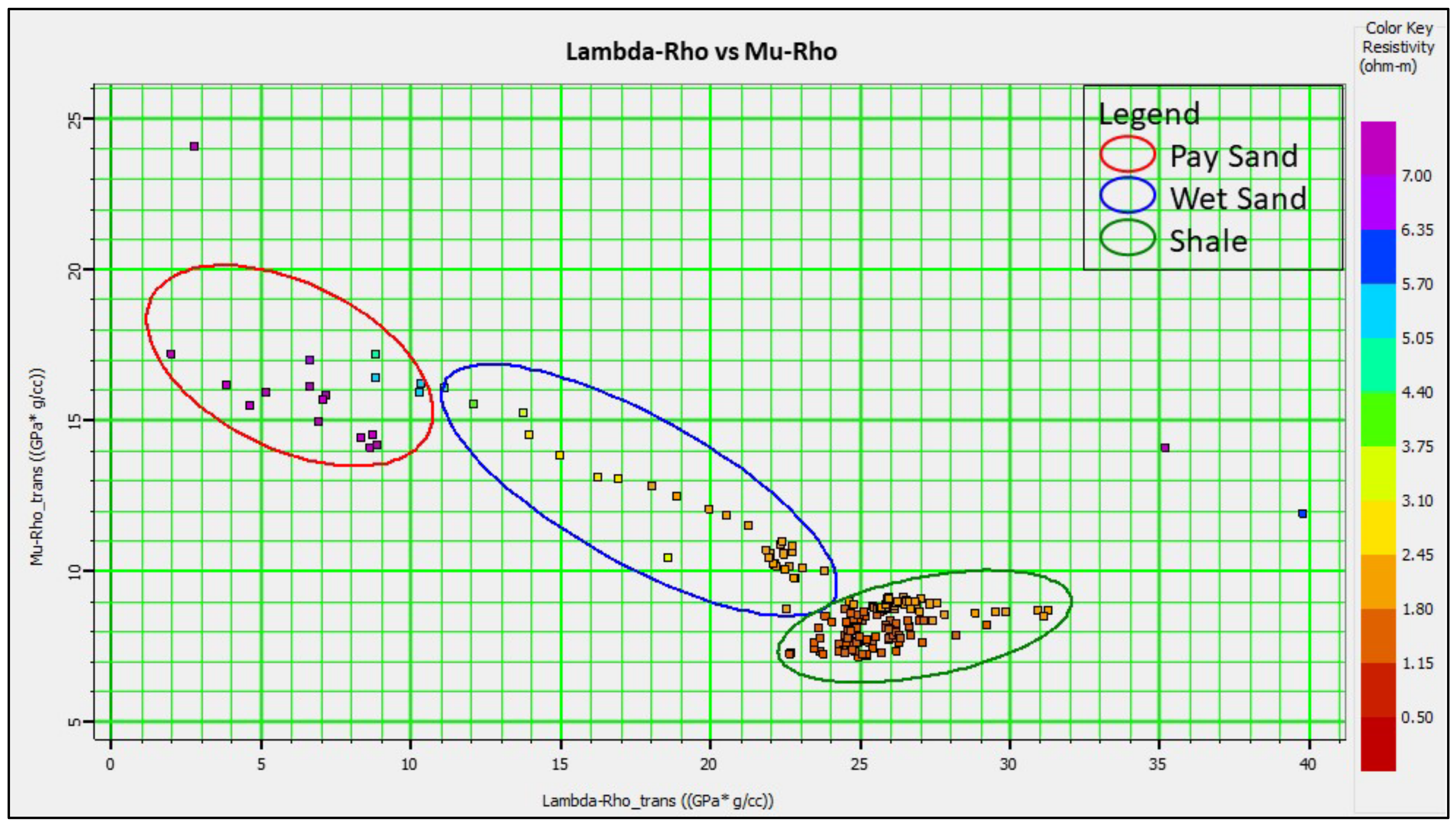
The cross-plot of μρ versus λρ presented in this study successfully distinguished the pay sand and shale in between Top H and H 60 horizons. From Figure 10, the pay sand is well characterised, occupying the low λρ and high μρ values in the red outline. This zone is also presented by the high resistivity data, an indication of hydrocarbon-filled sand. The wet sand is outlined in blue which most of the data within this zone fall within a medium range of λρ and μρ values. The distinguished wet sand also showed a good correlation to the lower resistivity values. The shale zone dominates the highest λρ and lowest μρ values in a green outline, related to the lowest measured resistivity shown from the resistivity colour scale.
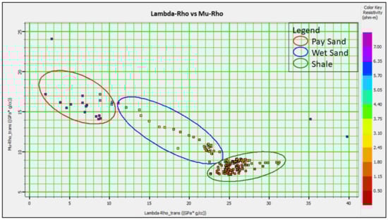
Figure 10.
Lambda-rho vs. Mu-rho cross plot with colour-coding based on resistivity for pay sand delineation.
The applicability of SQp and SQs attributes cross-plots in the reservoir characterisation is pioneered based on a study in Malay Basin to characterise clastic reservoirs [32]. It can be seen in Figure 11 that the HPHT reservoir in Sepat Field showed a clear distinction between pay sand, wet sand, and shale lithology. The pay sand in red outline, having high SQs and low SQp values, corresponds to the high formation resistivity around 8 Ωm of purple data. A decreasing SQs trend with slightly lower resistivity values is categorised as wet sand outlined in the blue circle. The decreasing value trends on SQs and resistivity on wet sand is a convenient observation. The two properties are sensitive to fluid change between hydrocarbon and water-filled zones. The shale zone is outlined in green showed an increasing trend of SQp values and decreasing SQs values. The shale zone also shows a good agreement to the low resistivity value of data indicating a rich clay-bound water-sediment that suppresses the resistivity measurement. Thus, the conducted cross-plot studies are capable of identifying the presence of hydrocarbons within the HPHT reservoir.
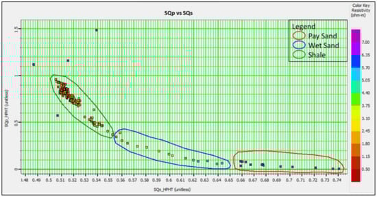
Figure 11.
SQp vs. SQs cross plot with colour-coding based on resistivity for pay sand delineation.
4.2. Pre-Stack Inversion
The pre-stack seismic inversion technique was used to invert the seismic data into four elastic properties, i.e., P-impedance, S-impedance, Vp/Vs ratio, and density.
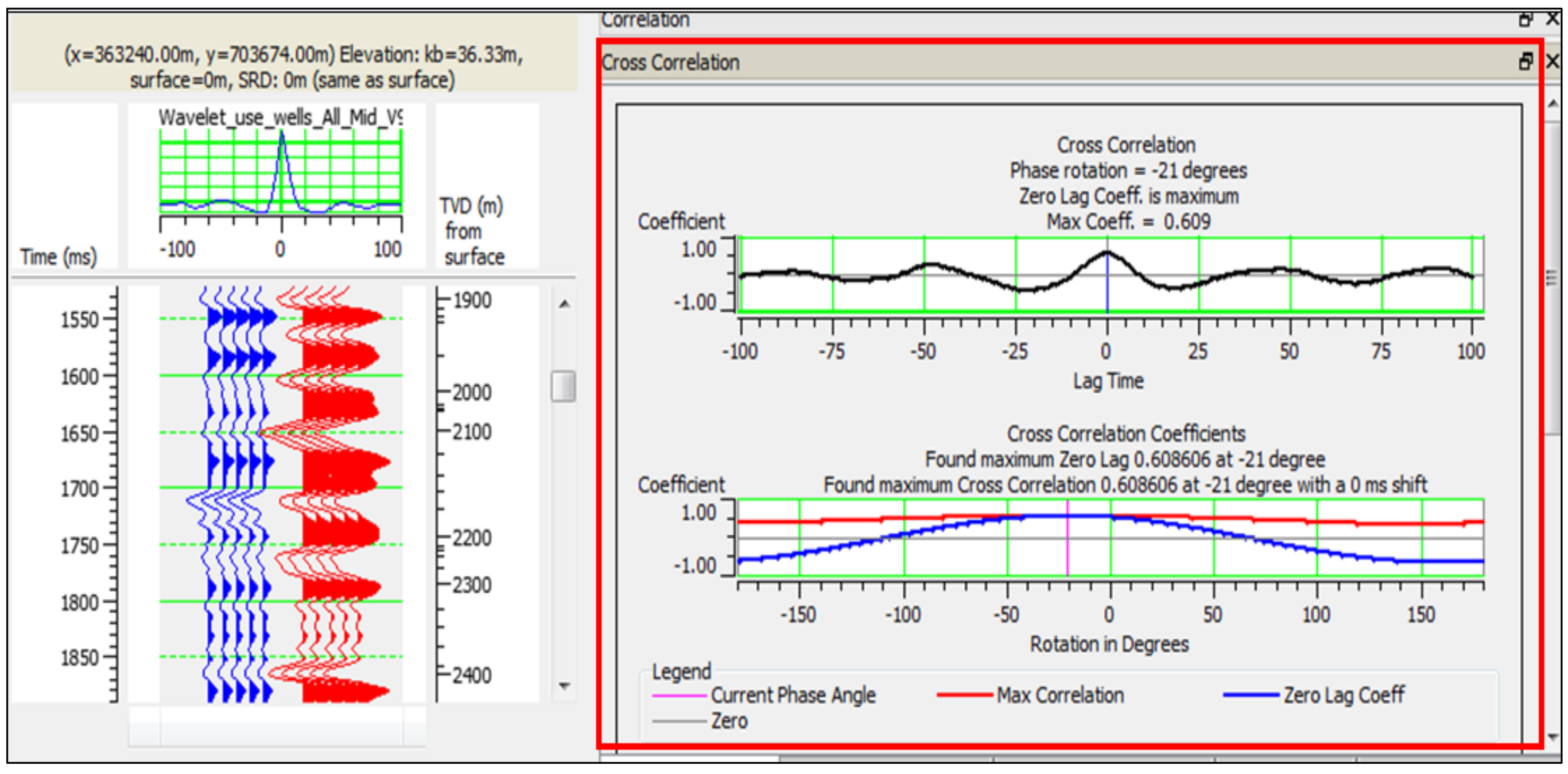
Figure 12 demonstrates the synthetic seismogram generated from the well log data and composite seismic traces extracted from seismic data at the well location. The correlation of 0.60 was achieved in the seismic-well ties process.
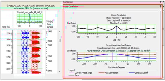
Figure 12.
Synthetic seismogram (blue) generated from the well log and composite seismic traces (red) extracted from seismic data at the well location. A correlation window is displayed in the red box.
The initial low-frequency models of P-wave, S-wave, Vp/Vs ratio and density were built based on seismic horizons and well data, as shown in Figure 13 and Figure 14. These models were then used as the input for the inversion process.

Figure 13.
Initial seismic model of (a) P-impedance and (b) S-impedance.
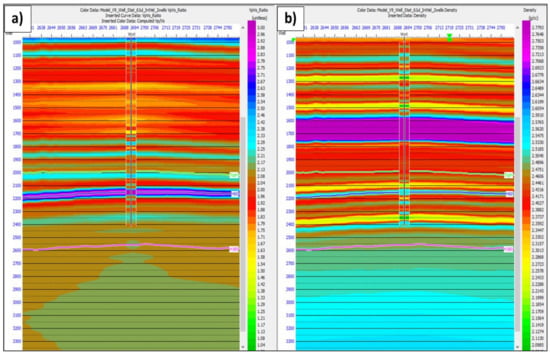
Figure 14.
Initial seismic model of (a) Vp/Vs ratio and (b) Density.
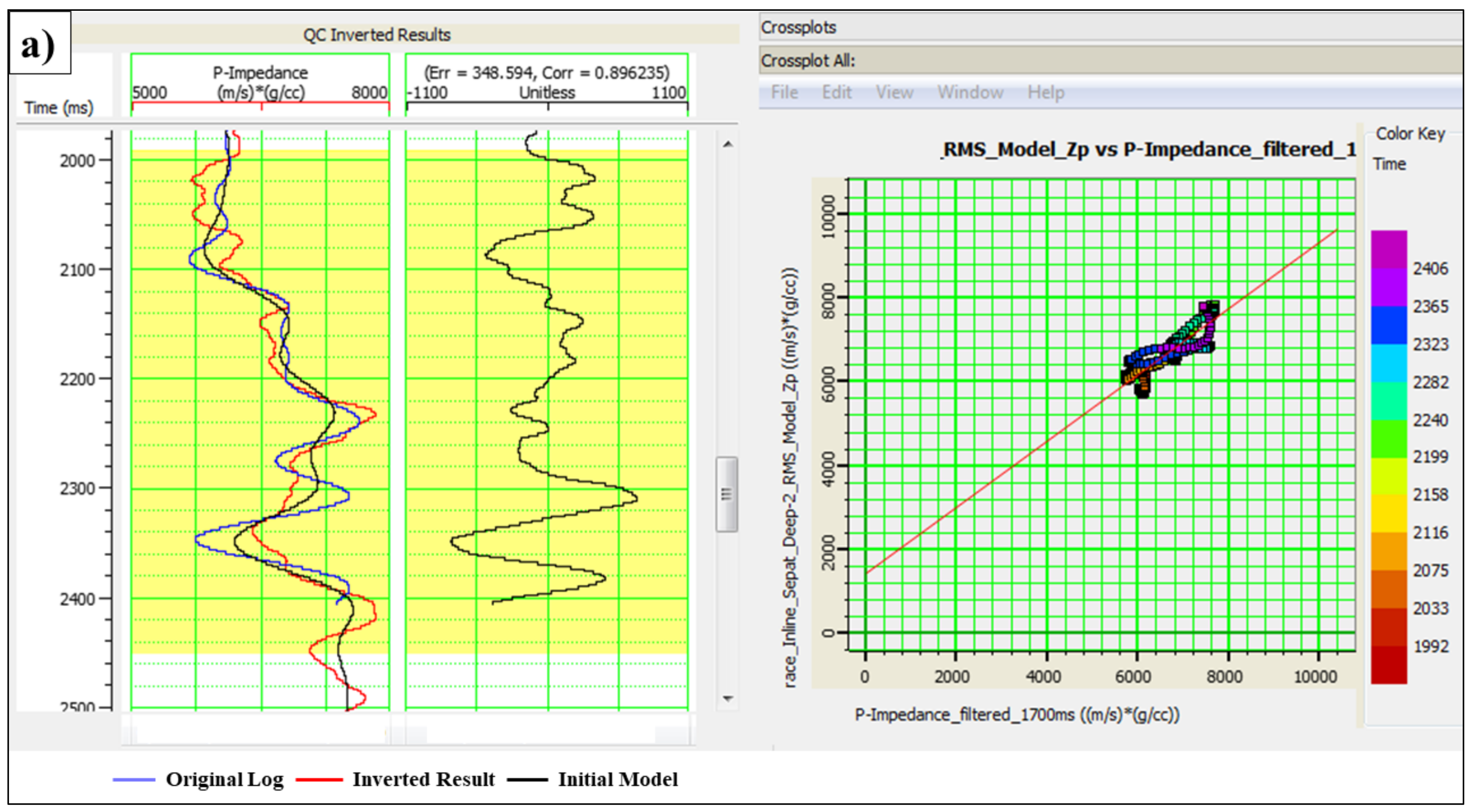
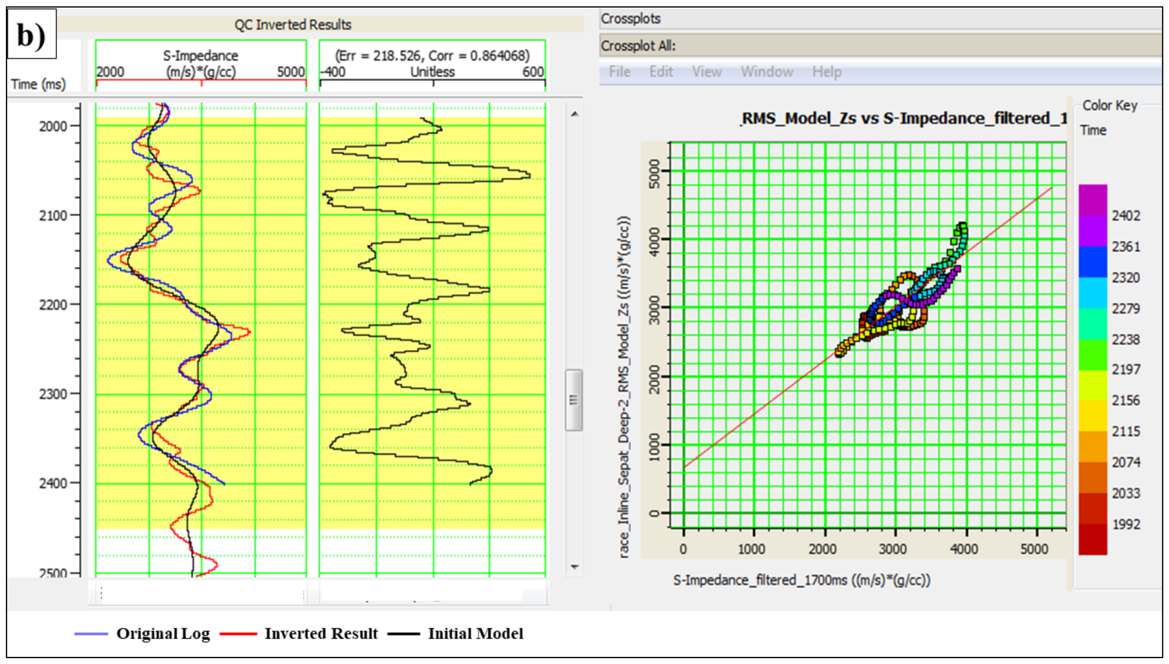
The inversion analysis at the well location of XD-2 well showed a good fit between inverted P-impedance, S-impedance, Vp/Vs ratio, and density with original well logs as seen in Figure 15 and Figure 16.
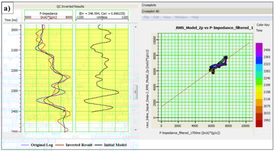
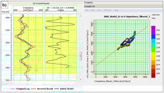
Figure 15.
(a) Simultaneous pre-stack inversion analysis plot for P-impedance property for well XD-2 within error calculation time window (yellow colour). The correlation between the original (blue) and inverted (red) P-impedance logs is 0.89. (b) Simultaneous pre-stack inversion analysis plot for S-impedance property for well XD-2 within error calculation time window (yellow colour). The correlation between the original (blue) and inverted (red) SI logs is 0.86.
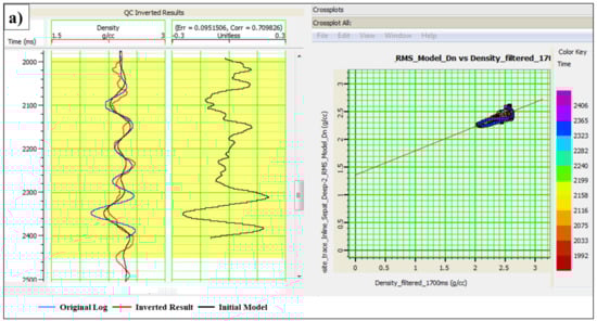
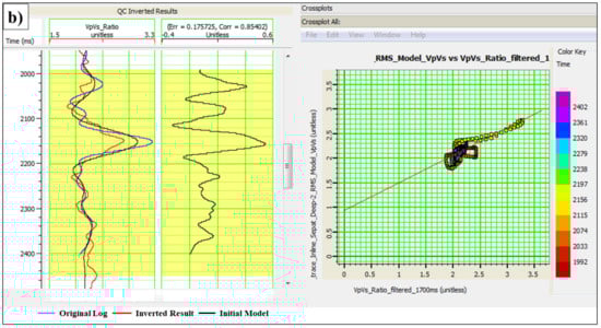
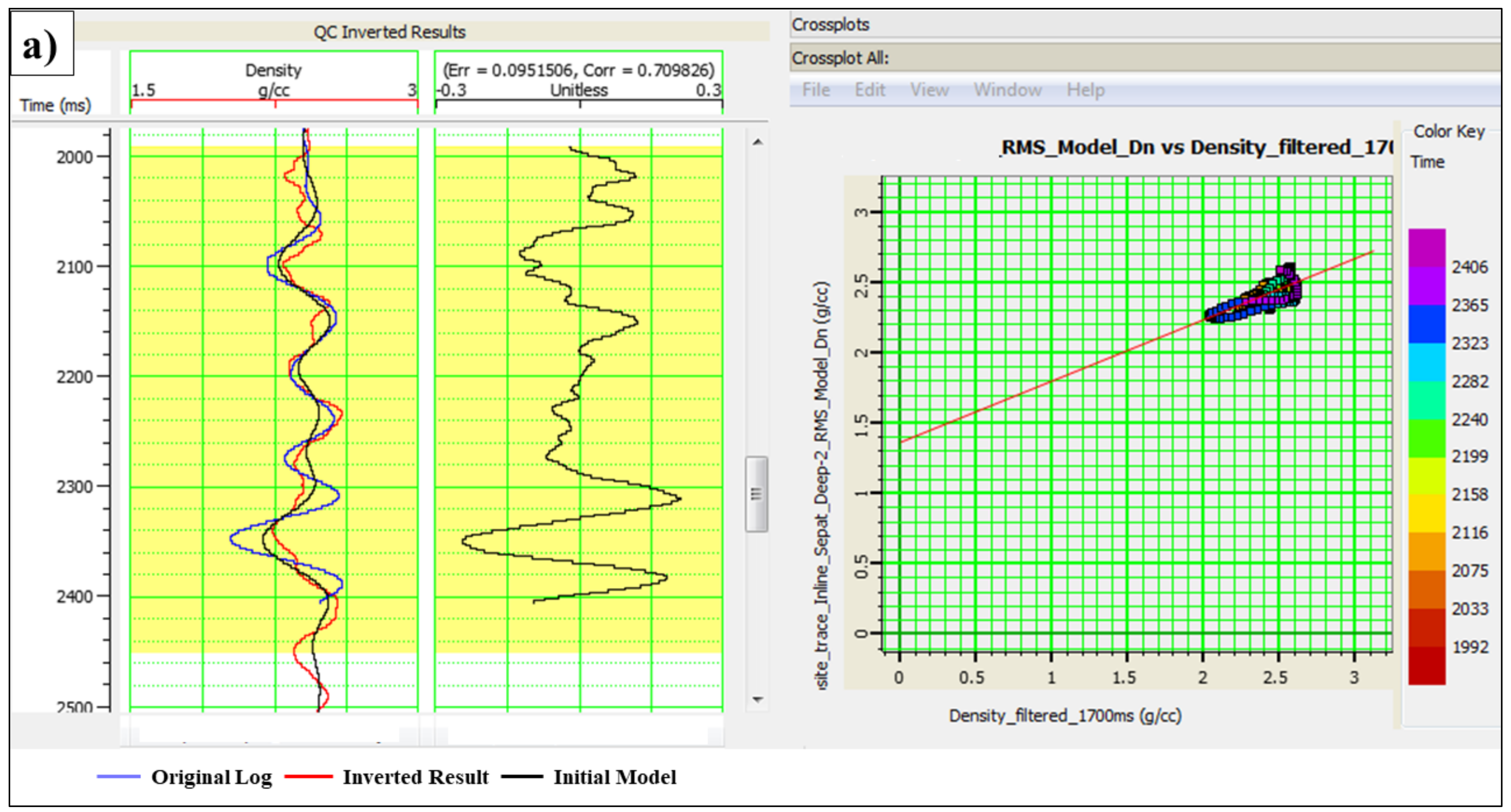
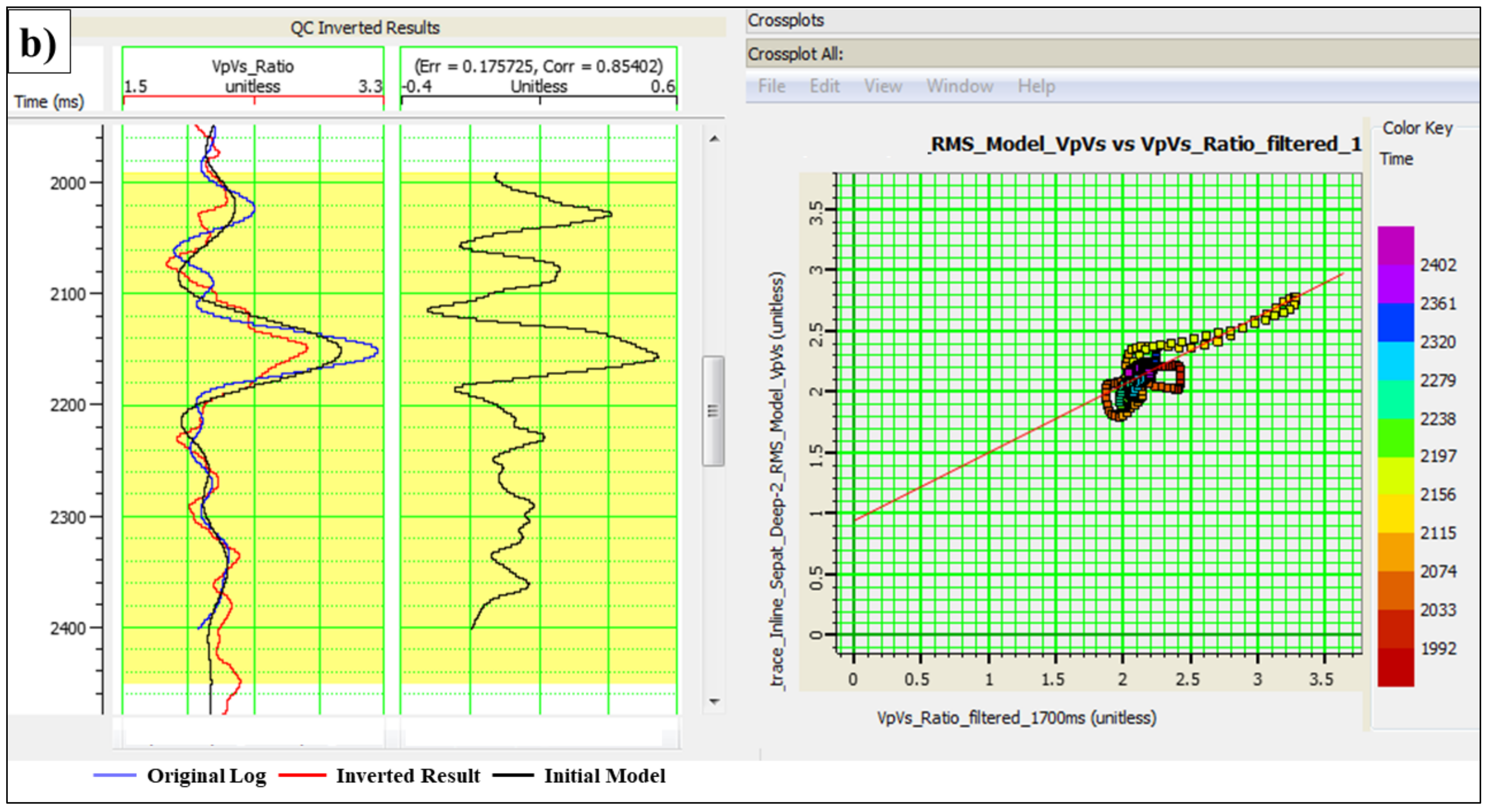
Figure 16.
(a) Simultaneous pre-stack inversion analysis plot for density property for well XD-2 within error calculation time window (yellow colour). The correlation between the original (blue) and inverted (red) density logs is 0.70. (b) Simultaneous pre-stack inversion analysis plot for Vp/Vs ratio property for well XD-2 within error calculation time window (yellow colour). The correlation between the original (blue) and inverted (red) Vp/Vs ratio logs is 0.85.
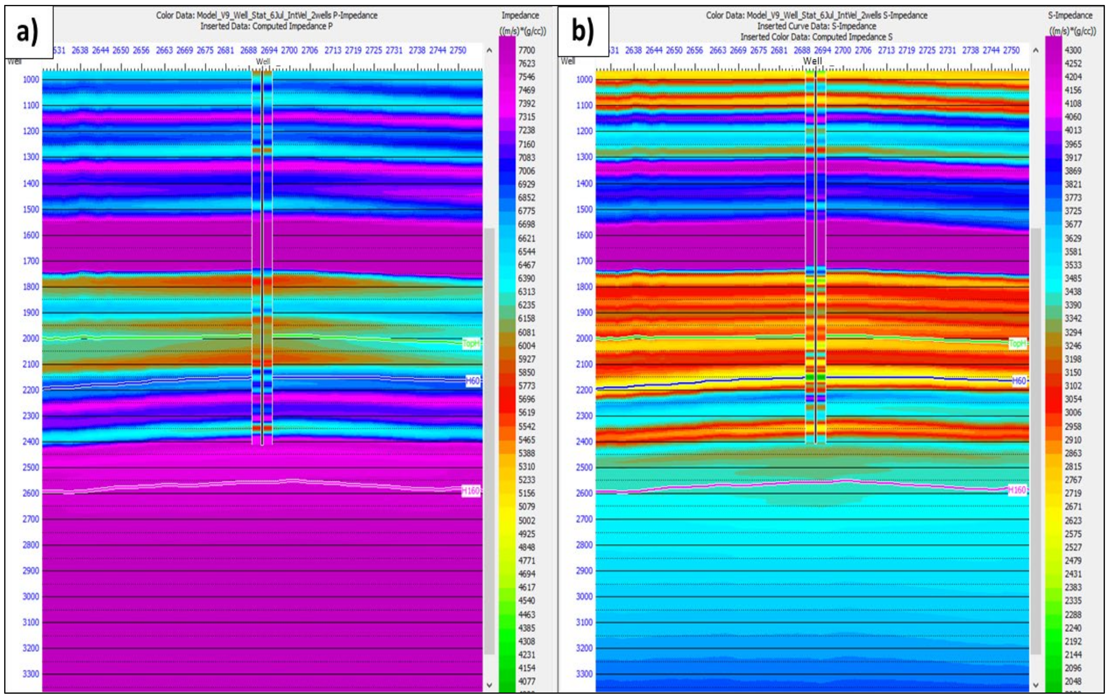
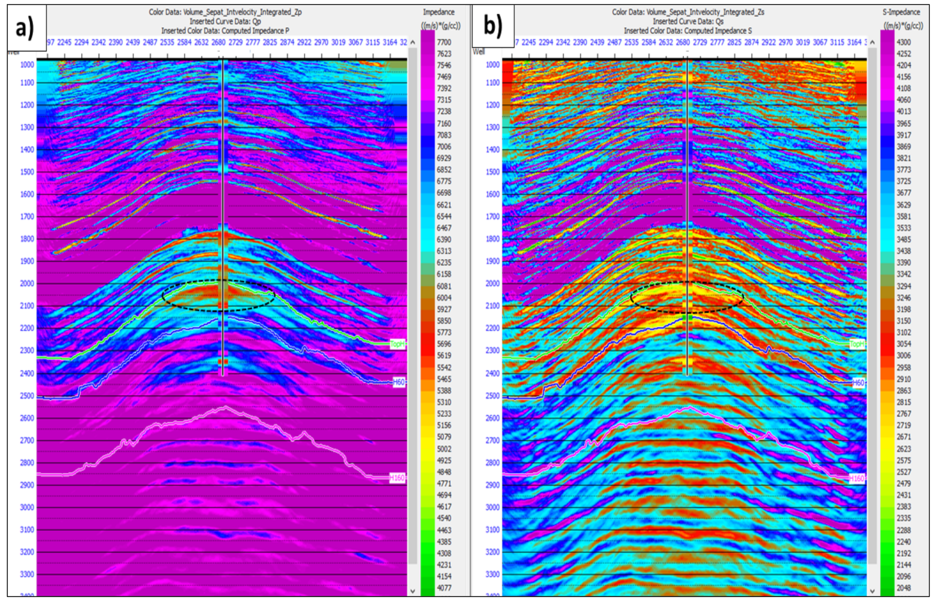
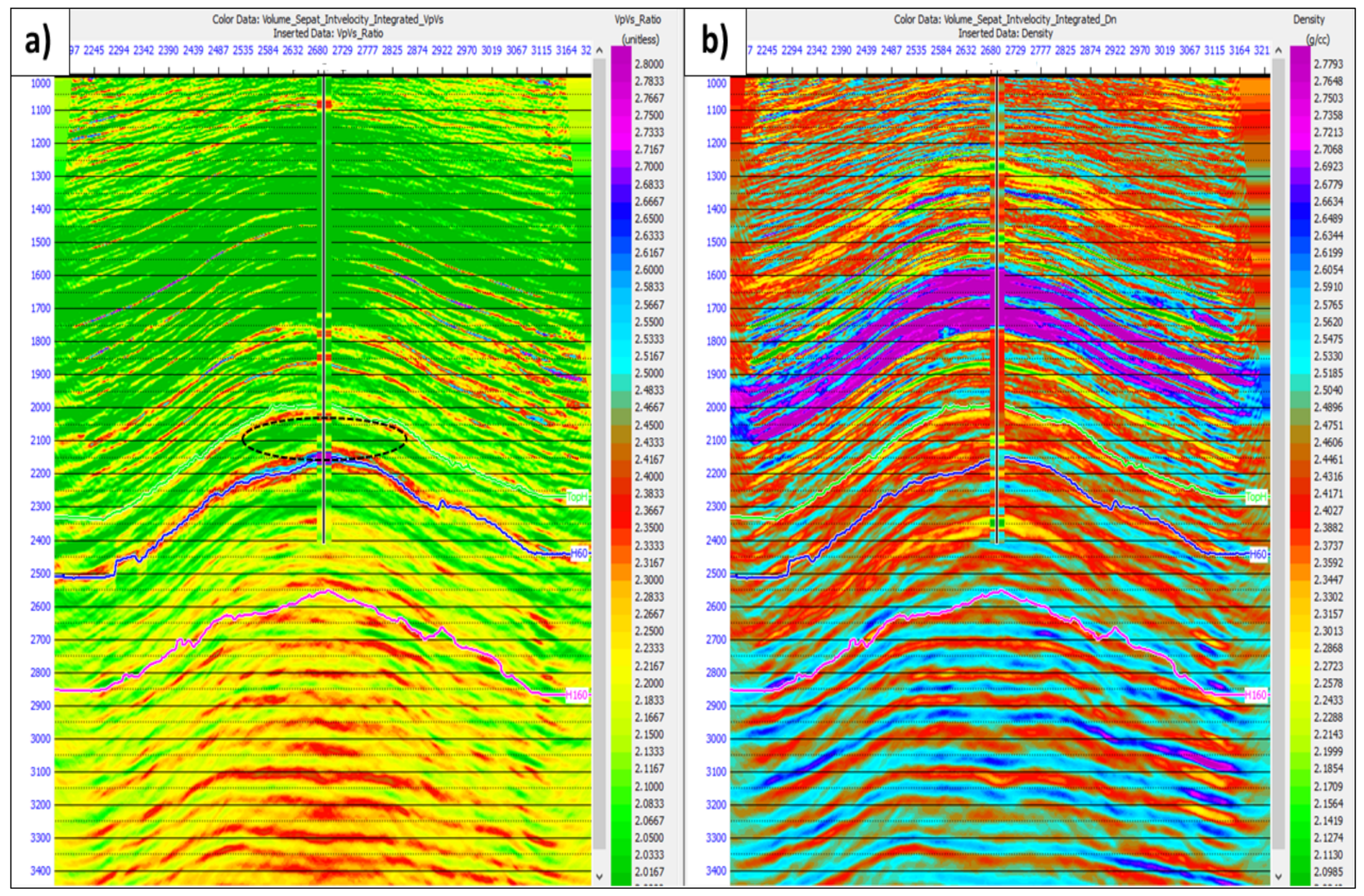
The inversion analysis showed a good match with the well data and aided in distinguishing possible reservoirs in the HPHT zone of the Sepat Field. Figure 17a,b illustrate the P-impedance and S-impedance inversion results with visible alternate layers of sand and shale. The low acoustic and shear impedance values ranging from 5600 to 6600 (m/s) × (g/cc) between Top H and H160 horizons represent the hydrocarbon-bearing sand. The Vp/Vs and density inversion results in Figure 18a,b also showed low values of Vp/Vs, and density (green intervals) may indicate the delineated hydrocarbon-bearing sand.
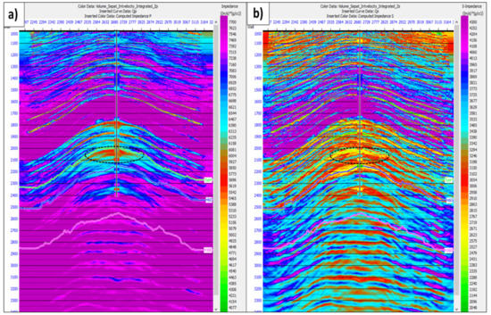
Figure 17.
(a) Inverted Zp crossline section containing XD-2 well from pre-stack simultaneous inversion; (b) Inverted Zs crossline section containing XD-2 well from pre-stack simultaneous inversion.
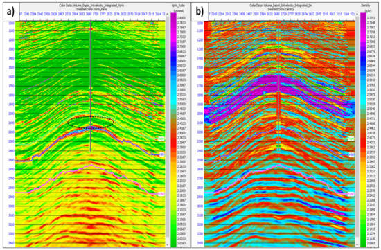
Figure 18.
(a) Inverted Vp/Vs ratio crossline section containing XD-2 well from pre-stack simultaneous in-version; (b) Inverted density crossline section containing XD-2 well from pre-stack simultaneous inversion.
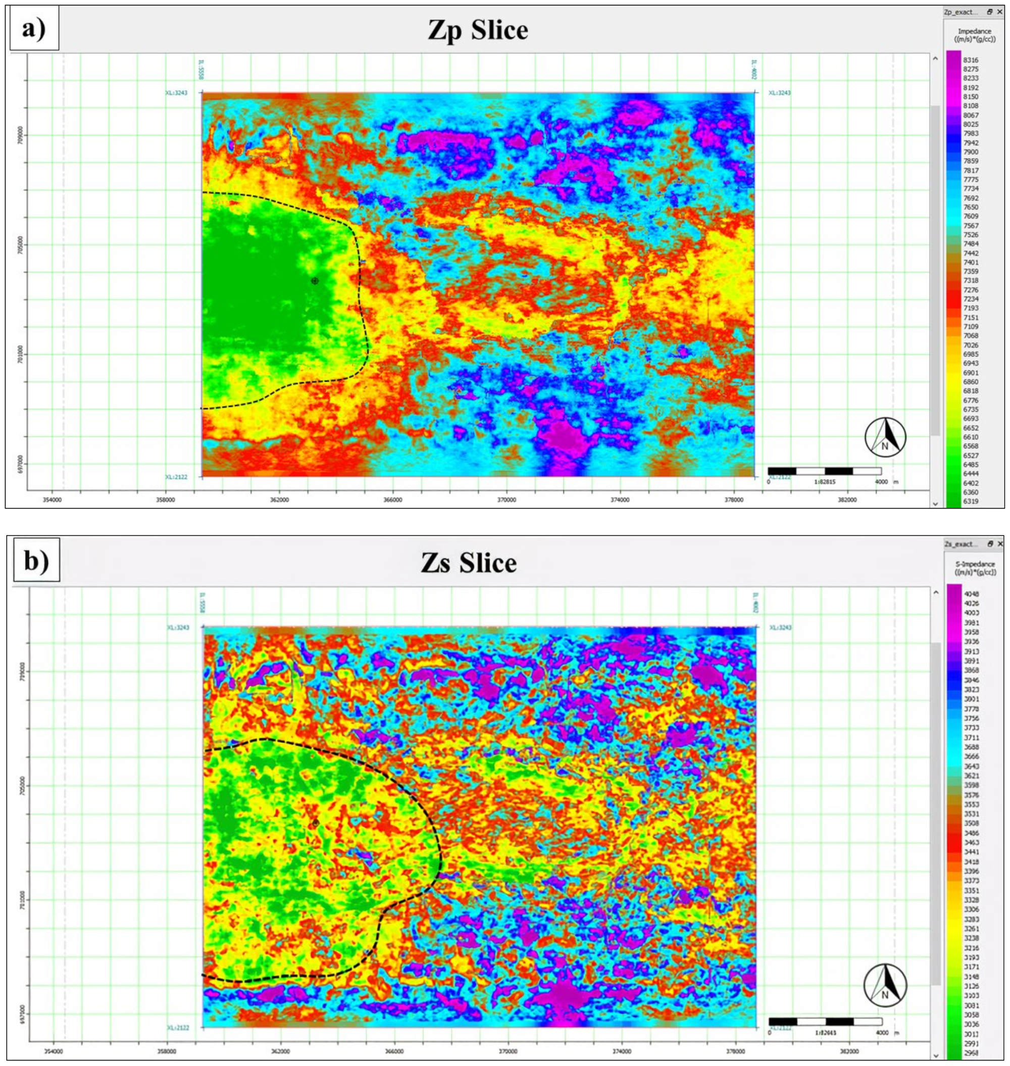
Horizon slices are generated using the data between Top H and H 60 horizons to observe the inversion results spatially. Horizon slices of Zp and Zs exhibited low responses of both impedances in the west of the study area, marked by the dotted line in Figure 19a,b. Low impedance responses in both Zp and Zs imply sand lithology filled by hydrocarbons, possibly gas. Eastwards, the impedance values increase, showing the lithological change of higher impedance, which is shale distribution. Density and Vp/Vs horizon slices in Figure 20a,b displayed the same trend as Zp and Zs horizon slices, which supported the interpretations made on both horizon slices of impedances.
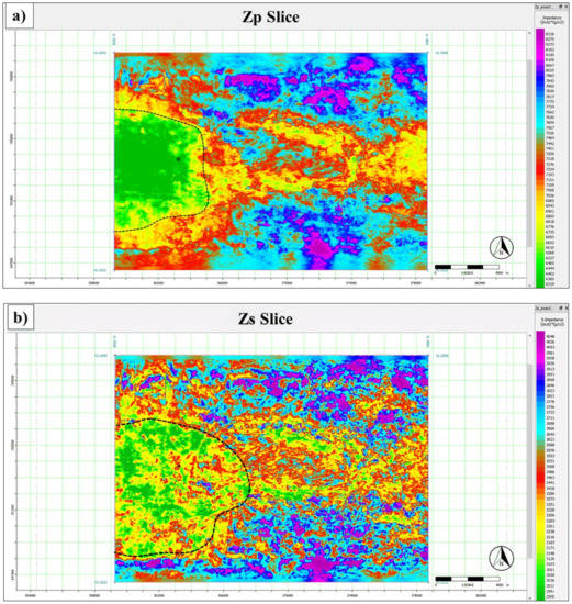
Figure 19.
(a) Averaged Zp data horizon slice within interval between Top H and H60 horizons; (b) Averaged Zs data horizon slice within interval between Top H and H60 horizons.
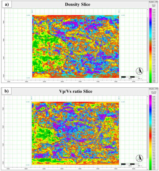
Figure 20.
(a) Averaged density data horizon slice within an interval between Top H and H60 horizons; (b) Averaged Vp/Vs ratio data horizon slice within an interval between Top H and H60 horizons.
The low response of Vp/Vs in the horizon slice (Figure 20b) is due to the increase in Vs and reduction in Vp. A surge in Vs is the reduction in density and the increasing absorption of distortion by free gas in pores. On the other hand, the reduction in Vp is due to decreasing the bulk modulus of reservoir rocks, compensating for lessening rock density. The low response of Vp/Vs in the horizon slice indicates the presence of hydrocarbons, as the bulk modulus of hydrocarbons reduces the Vp and rises the Vs through porous rocks. Additionally, there is a reduction in density as the water in rock is replaced by hydrocarbons.
4.3. SQp and SQs Attributes
The outcomes of pre-stack simultaneous inversion, Vp/Vs, and density 3D cubes are implemented to generate SQp and SQs through mathematical equations. As discussed earlier, the SQp attribute has a similar log response to the gamma-ray log, and SQs is close to the resistivity log response. They are proven to be effective in litho-fluid delineation.
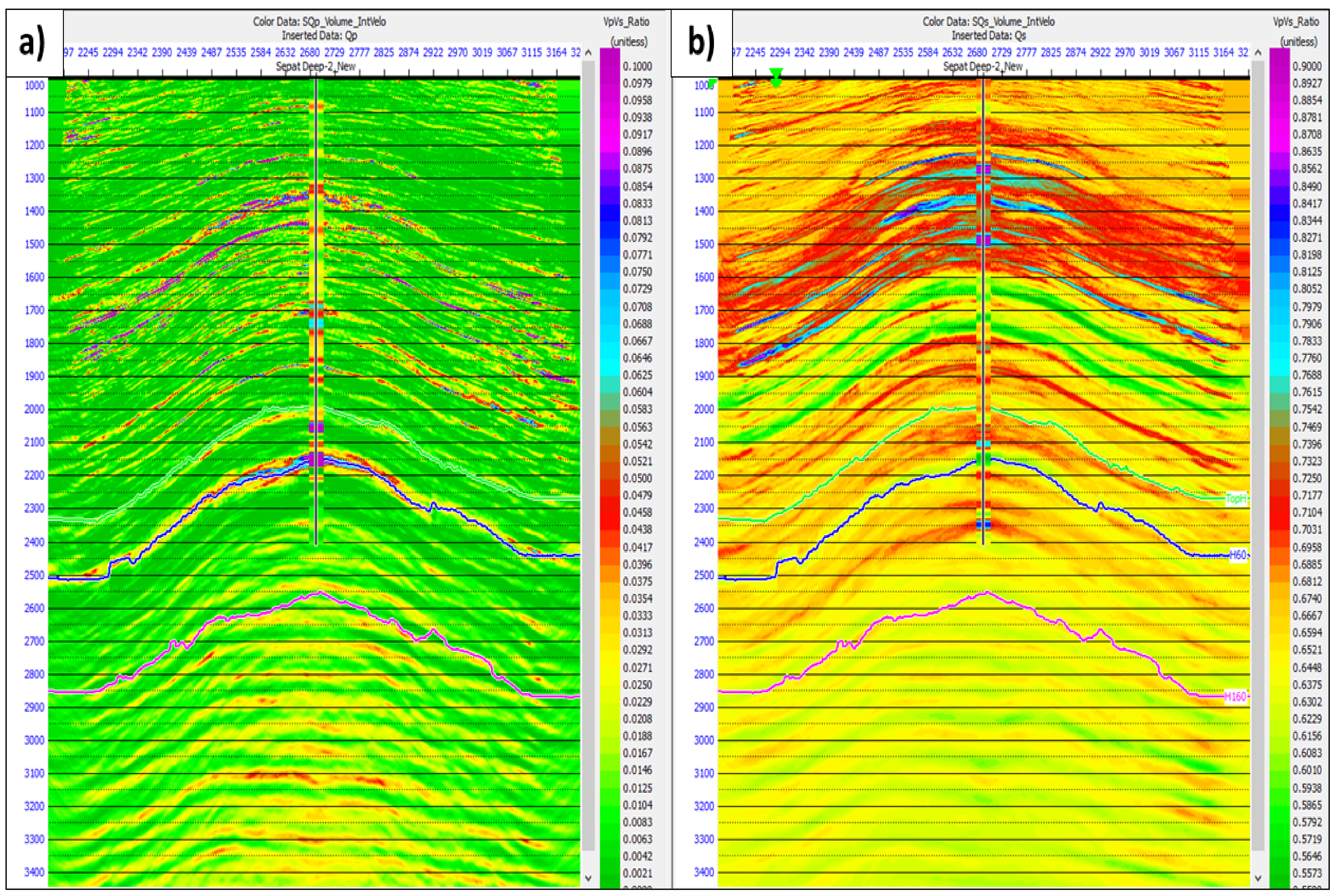
The hydrocarbon-bearing zones and their continuity can be identified in SQp and SQs sections (Figure 21a,b). The reservoir target between Top H and H60 horizon demonstrates low SQp and high SQs values. The SQp values range between 0.0021 and 0.04, and SQs values range from 0.62 to 0.73 in possible hydrocarbon-bearing sands intervals.
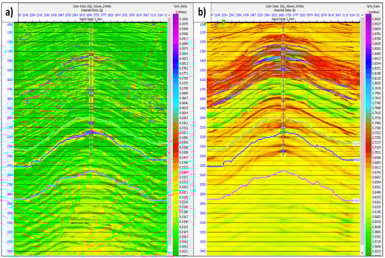
Figure 21.
(a) Inverted SQp crossline section containing XD-2 well; (b) Inverted SQs crossline section containing XD-2 well.
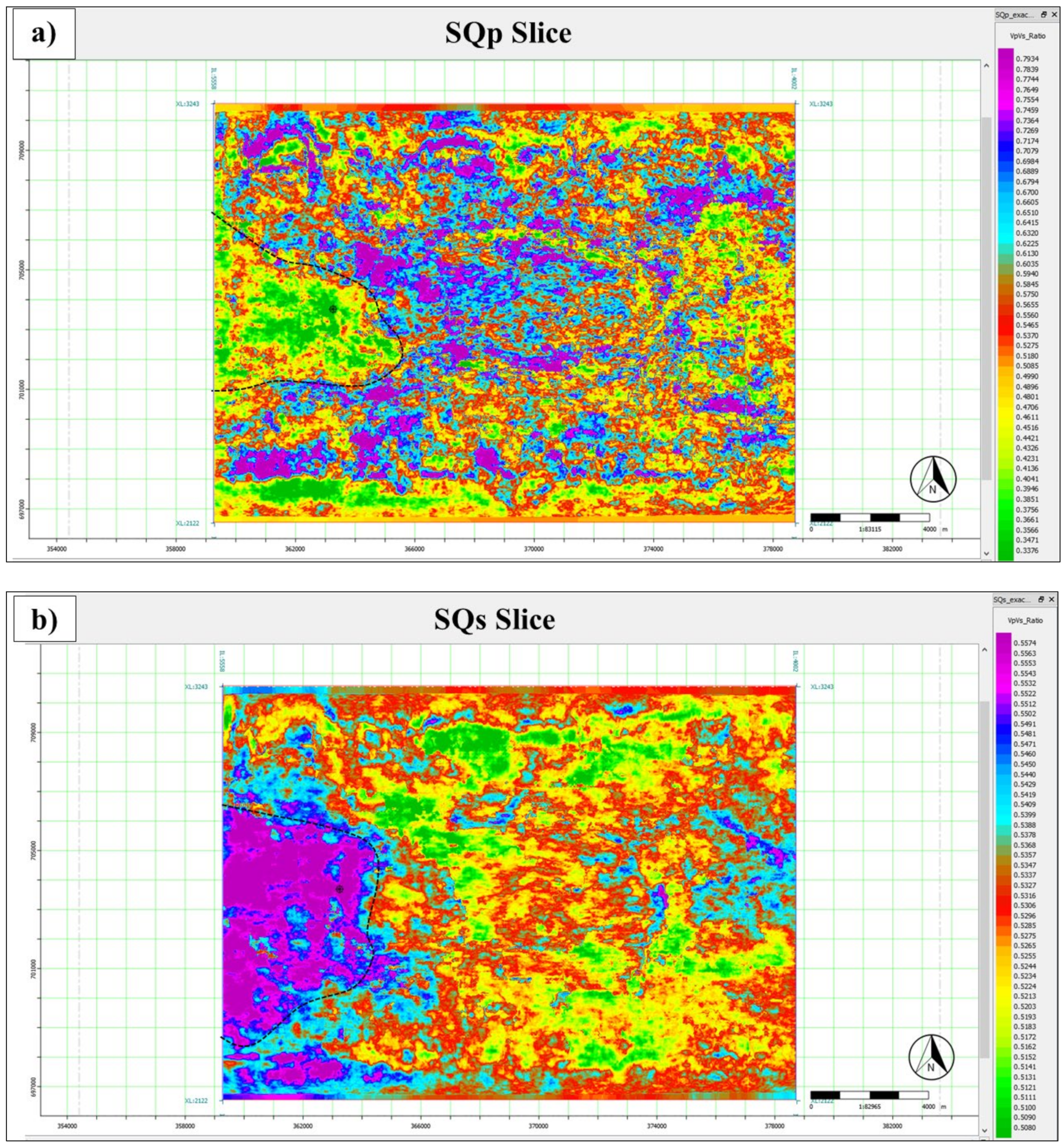
Figure 22a,b show the distribution and changes of SQp and SQs attributes’ values within the interval between Top H and H60 horizons. The SQp attributes delineated the distribution of sand (green colour) and shale (violet colour) lithology. The area of interest (dotted line in Figure 22a) responded as a low value of the SQp attribute, indicating the presence of sand lithology. The dotted line in Figure 22b exhibited a high SQs value, indicating the sand porosity is filled by hydrocarbons. From the horizon slices generated at Top H to H 60 horizons of the study area, it can be summarised that the west of the study area is sand-prone and filled by hydrocarbons.
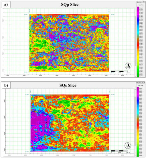
Figure 22.
(a) Averaged SQp data horizon slice within an interval between Top H and H60 horizons; (b) Averaged SQs data horizon slice within an interval between Top H and H60 horizons.
4.4. Artificial Neural Network (ANN)
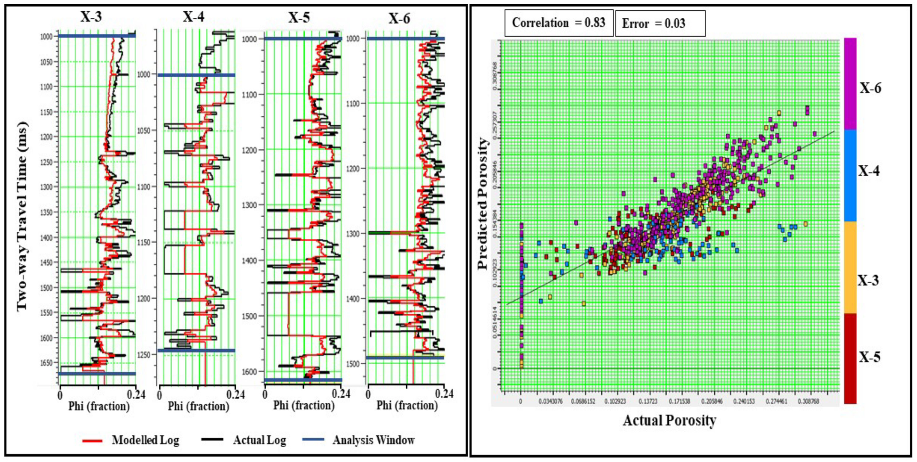
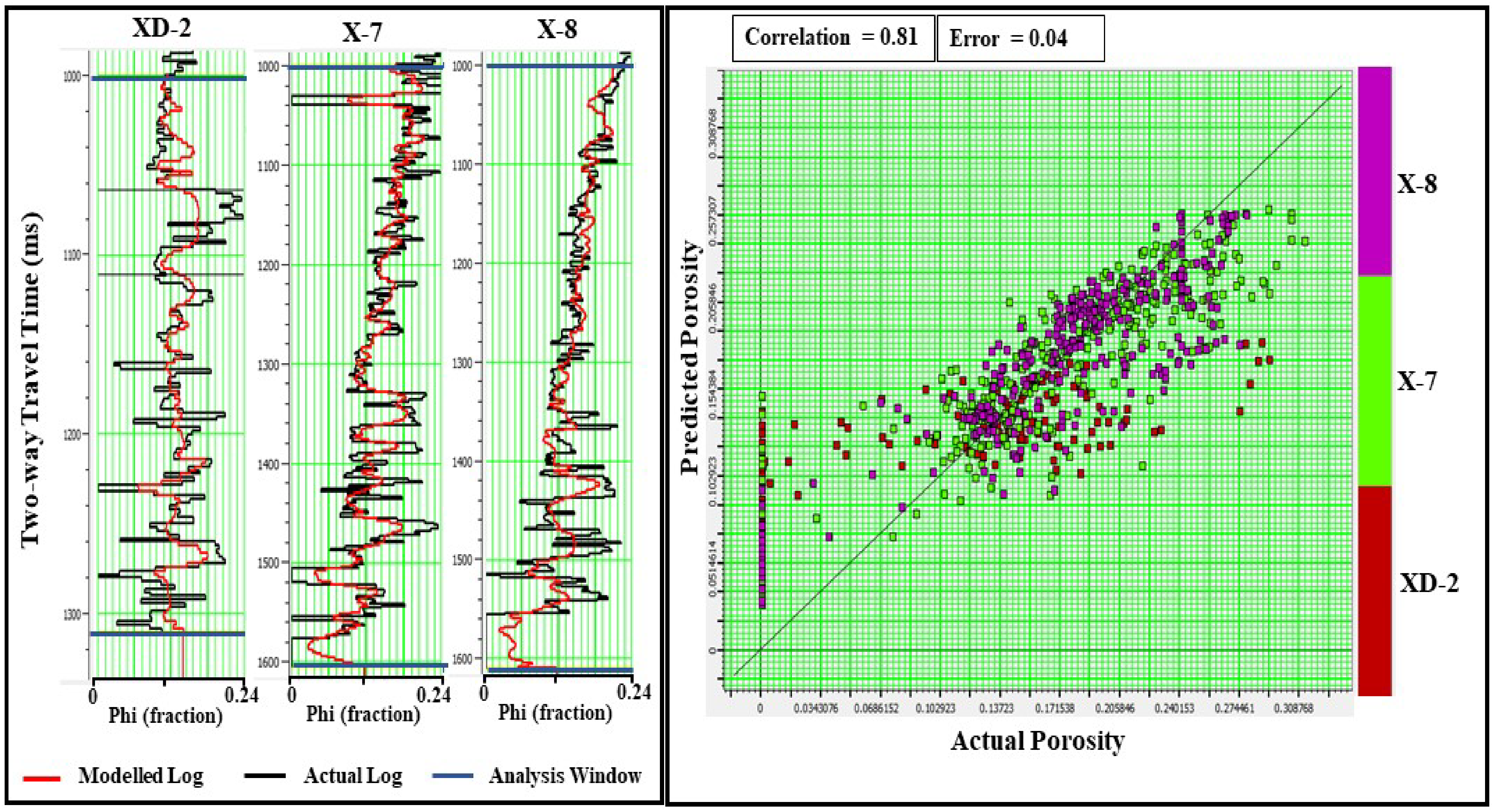
The RBFN model is trained with an expected outcome, such as porosity using well-log and seismic data to create an appropriate range of weights between nodes. As training wells, X-3, X-4, X-5, and X-6 wells are used, while X-7, X-8, and XD-2 wells are retained to validate the predicted results. In the RBFN model, the sigma value is 0.1 for estimating porosity with a different time window of each well. The time windows are 1000–1650 ms at X-3, 1000–1250 ms at X-4, 1000–1650 ms at X-5, and 1000–1490 ms at X-6, which is considered for the study of training error. For validation error analysis, the time windows are 1000–1320 ms at XD-2, 1000–1600 ms at X-7, and 1000–1620 ms at X-8. The training dataset is used for modelling, while the validation dataset determines its prediction error. Figure 23 demonstrates the training error analysis window for X-3, X-4, X-5, and X-6 wells, while the validation error analysis window for porosity prediction is shown in Figure 24 for XD-2, X-7, and X-8 wells.
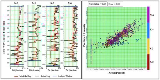
Figure 23.
The error analysis window for ANN training demonstrates a 0.03 training error and a 0.83 correlation between the true and estimated porosity.
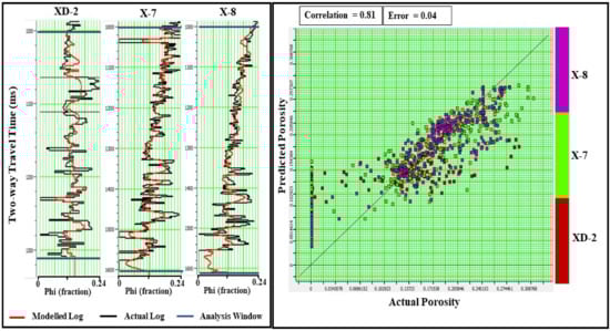
Figure 24.
The error analysis window for ANN validation demonstrates a 0.04 validation error and 0.81 correlation between the true and estimated porosity.
The trained-porosity from ANN demonstrates a 0.03 training error and a 0.83 correlation between the true and trained-porosity (Figure 23). The predicted porosity is validated with a correlation of 0.81 and an error of 0.04 of the RBFN model (Figure 24). The predicted porosity consistently correlates with the values obtained from the log, equally in well locations for training and validation.
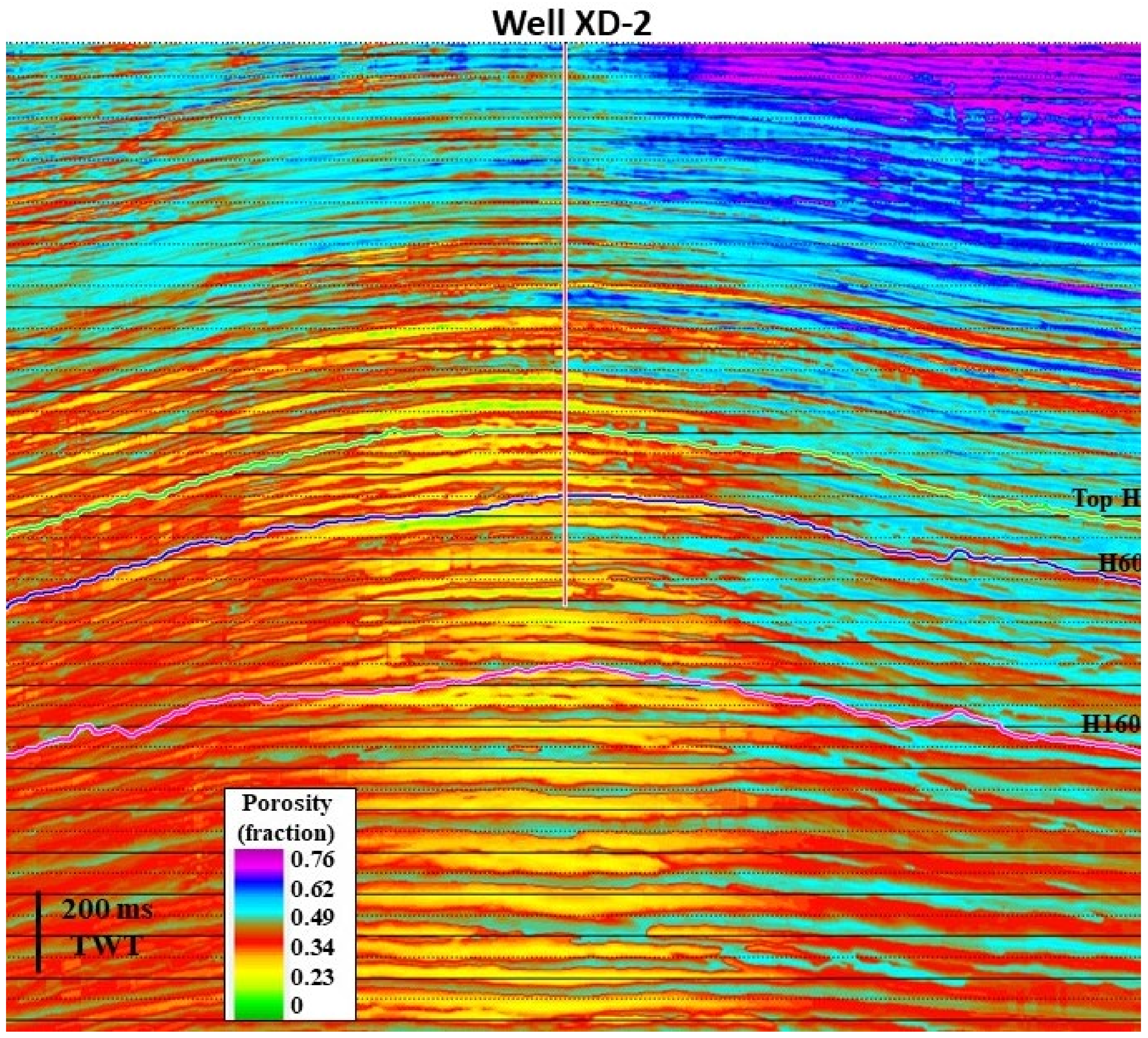
Furthermore, to generate a 3D volume of porosity, the validated RBFN porosity model was applied to the 3D seismic data. The RBFN porosity-derived volume ranges from 23% to 76%, as shown in Figure 25.
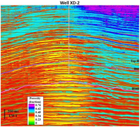
Figure 25.
ANN predicted porosity crossline section containing Top H, H60, and H160 horizons and XD-2 well.
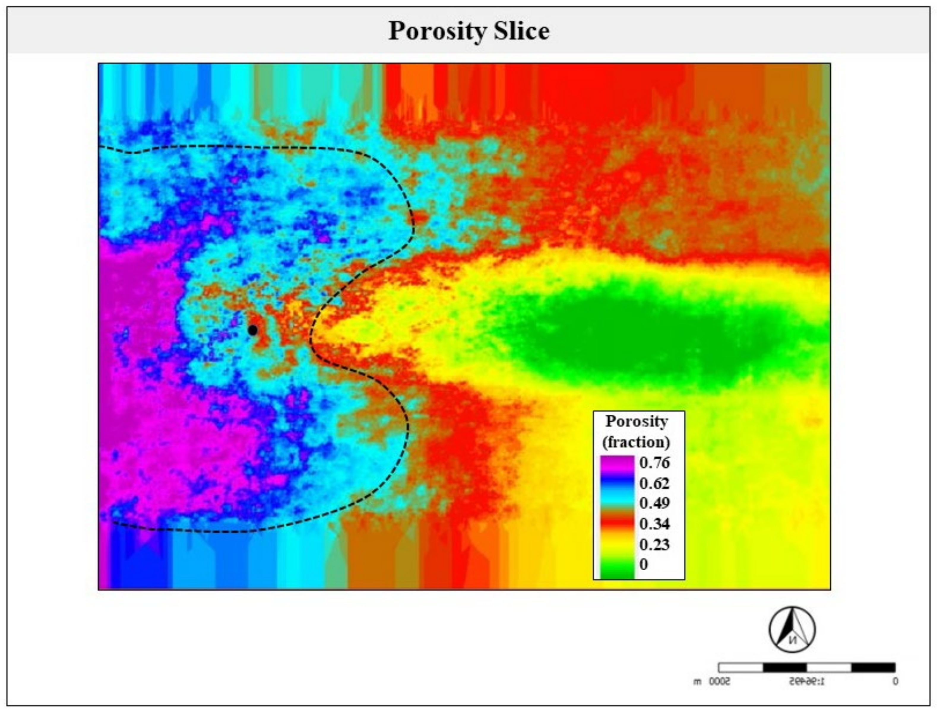
Figure 26 shows the spatial changes of porosity data within the zone of interest (between Top H and H60 horizons). The area of interest (dotted line in Figure 26) responded as a high porosity value, indicating the HPHT reservoir with possible hydrocarbon fluids.

Figure 26.
Averaged porosity data horizon slice within interval between Top H and H60 horizons.
5. Conclusions
The HPHT field is a complicated field to be explored. Progressive preparation is a significant aspect for successful exploration, and modified techniques should be regularly occupied to address the HPHT concerns. The HPHT zone conditions the drilling of wells in many circumstances, for instance, the high temperature caused the slurry to become sensitive, so the setting time of slurry is extremely lessened, causing the cement to thicken quicker than in normal temperature wells. High pressure, on the other hand, has consequences on both the well and drilling fluid. If the pressure is not being predicted appropriately, the designated casing will not be capable of enduring the formation pressure, leading to a breakdown of the casing in the well and, thus, causing a kick.
This study utilized the integration of several techniques to characterise the reservoir properties of the HPHT zone in the Sepat field. The workflow involved techniques of rock physics study, pre-stack seismic inversion, SQp and SQs attributes and ANN application for a clastic environment. The Lamé constant and shear modulus are more sensitive to variations in porosity and lithology and allow for more accurate reasoning about filling in pore spaces than P- and S-impedances alone. The interpreter was able to identify the most prospective zones inside the sequence by extracting and analysing inversion attributes. SQp and SQs attributes provided us with the information about sand and shale lithology and fluid distribution. Furthermore, the application of 3D models consisting of P-impedance, S-impedance, density, Vp/Vs ratio, and SQp, SQs attributes as the main input for ANN modelling allowed obtaining insight into the distribution of porosity in HPHT zone of Sepat field.
The integrated approach succeeded to predict rock properties and reservoir porosity away from the well in the HPHT zone of the Sepat field. The results suggested that the one possible reservoir is identified, located in between the Top H and H 60 horizons on the west of the study area at the location of XD-2 well. Visible alternate layers of sand and shale are observed in the study area. The sandy reservoirs in the HPHT zone are characterized by porosity ranging from 23% to 76% within 2000 to 2900 ms. The usage of novel SQp and SQs attributes as input for ANN modelling proved its effectiveness in improving the lateral continuity of the porosity prediction related to delineated lithology and fluid distribution. By characterising the reservoir properties away from wells in the HPHT zone, it is hoped that the oil and gas industry can drive the limits to deeper depths and in hotter wells in the continuing exploration for new sources of hydrocarbons.
Author Contributions
Conceptualisation, G.Y., N.N.A.A.N.M.H. and N.F.S.; methodology, G.Y., N.N.A.A.N.M.H. and N.F.S.; software, G.Y., N.N.A.A.N.M.H. and N.F.S.; validation, G.Y., N.N.A.A.N.M.H. and N.F.S.; formal analysis, G.Y., N.N.A.A.N.M.H. and N.F.S.; investigation, G.Y., N.N.A.A.N.M.H. and N.F.S.; resources, M.H.; data curation, G.Y., N.N.A.A.N.M.H. and N.F.S.; writing—original draft preparation, G.Y.; writing—review and editing, N.N.A.A.N.M.H., N.F.S., M.H. and H.S.; visualisation, G.Y., N.N.A.A.N.M.H. and N.F.S.; supervision, M.H. and H.S.; project administration, M.H.; funding acquisition, M.H. All authors have read and agreed to the published version of the manuscript.
Funding
This research was funded by UTP fundamental research grant with grant number 015LCO-348.
Institutional Review Board Statement
Not applicable.
Informed Consent Statement
Not applicable.
Acknowledgments
Authors express their gratitude to the Centre of Seismic Imaging (CSI) at University Technology PETRONAS for valuable resources, facilities and funding. This research was made possible by a UTP fundamental research grant with cost centre 015LCO-348. We acknowledge PETRONAS for providing the data, CGG company for providing HampsonRussell software and Schlumberger company for providing PETREL software for this research.
Conflicts of Interest
The authors declare no conflict of interest.
References
- Journel, A.G. Geology and Reservoir Geology. Stochastic Modeling and Geostatistics; Yarus, J.M., Chambers, R.L., Eds.; AAPG Computer Applications in Geology: Tulsa, OK, USA, 1995; pp. 19–20. [Google Scholar]
- Al-hasani, A.; Hakimi, M.H.; Saaid, I.M.; Salim, A.M.A.; Mahat, S.Q.A.; Ahmed, A.A.; Umar, A.A.B. Reservoir characteristics of the Kuhlan sandstones from Habban oilfield in the Sabatayn Basin, Yemen and their relevance to reservoir rock quality and petroleum accumulation. J. Afr. Earth Sci. 2018, 145, 131–147. [Google Scholar] [CrossRef]
- Das, B.; Chatterjee, R. Well log data analysis for lithology and fluid identification in Krishna-Godavari Basin, India. Arab. J. Geosci. 2018, 11, 231. [Google Scholar] [CrossRef]
- Schultz, P.S.; Ronen, S.; Hattori, M.; Corbett, C. Seismic-guided estimation of log properties Part 1: A data-driven interpretation methodology. Lead. Edge 1994, 13, 305–310. [Google Scholar] [CrossRef]
- Saikia, P.; Baruah, R.D.; Singh, S.K.; Chaudhuri, P.K. Artificial Neural Networks in the domain of reservoir characterization: A review from shallow to deep models. Comput. Geosci. 2020, 135, 104357. [Google Scholar] [CrossRef]
- Babasafari, A.A.; Ghosh, D.P.; Salim, A.M.A.; Kordi, M. Integrating petroelastic modeling, stochastic seismic inversion, and Bayesian probability classification to reduce uncertainty of hydrocarbon prediction: Example from Malay Basin. Interpretation 2020, 8, SM65–SM82. [Google Scholar] [CrossRef]
- Gogoi, T.; Chatterjee, R. Estimation of petrophysical parameters using seismic inversion and neural network modeling in Upper Assam basin, India. Geosci. Front. 2018, 10, 1113–1124. [Google Scholar] [CrossRef]
- Smithson, T. The Defining Series: HPHT Wells; Oilfield Review; Schlumberger: Houston, TX, USA, 2016. [Google Scholar]
- Shadravan, A.; Amani, M. HPHT 101—What every engineer or geoscientist should know about high pressure high temperature wells. In Proceedings of the SPE Kuwait International Petroleum Conference and Exhibition, Kuwait City, Kuwait, 10–12 December 2012; Volume 2, pp. 917–943. [Google Scholar] [CrossRef]
- He, W.; Hao, J.; Yang, J.; Guan, X.; Dai, R.; Li, Y. Application of pre-stack simultaneous inversion to predict gas-bearing dolomite reservoir: A case study from Sichuan Basin, China. Carbonates Evaporites 2019, 34, 1191–1201. [Google Scholar] [CrossRef]
- Francis, A. A Simple Guide to Seismic Inversion. GeoExPro 2013, 10, 46–50. [Google Scholar]
- Verma, A.K.; Cheadle, B.A.; Routray, A.; Mohanty, W.K.; Mansinha, L. Porosity and Permeability estimation using neural network approach from well log data. In Proceedings of the SPE Annual Technical Conference and Exhibition, San Antonio, TX, USA, 8–10 October 2012. [Google Scholar]
- Madon, M. Petroleum Geology and Resources of Malaysia; Petronas: Kuala Lumpur, Malaysia, 1999. [Google Scholar]
- Uttarathiyang, T.; Pigott, J.D. New Unexplored Thailand Basin Frontier: North Malay Basin Post Rift Oligocene Deltas. In Proceedings of the International Symposia on Geoscience and Environments of Asian Terranes (GREAT 2008), 4th IGCP 516 and 5th APSEG, Bangkok, Thailand, 24–26 November 2008; pp. 370–373. [Google Scholar]
- Kumar, M.; Dasgupta, R.; Singha, D.K.; Singh, N.P. Petrophysical evaluation of well log data and rock physics modeling for characterization of Eocene reservoir in Chandmari oil field of Assam-Arakan basin, India. J. Pet. Explor. Prod. Technol. 2018, 8, 323–340. [Google Scholar] [CrossRef] [Green Version]
- Goodway, B.; Chen, T.; Downtown, J. Improved AVO fluid detection and lithology discrimination using Lame petrophysical parameters. In Proceedings of the 67th Annual international Meeting, SEG, Expanded Abstracts, Dallas, TX, USA, 2–7 November 1997; pp. 183–186. [Google Scholar]
- Perez, M.A.; Tonn, R. Reservoir Modelling and Interpretation with Lamé’s Parameters: A Grand Banks Case Study; EnCana Corporation: Calgary, AB, Canada, 2003; pp. 1–11. [Google Scholar]
- Hermana, M.; Ngui, J.Q.; Sum, C.W.; Ghosh, D.P. Feasibility Study of SQp and SQs Attributes Application for Facies Classification. Geosciences 2018, 8, 10. [Google Scholar] [CrossRef] [Green Version]
- Varatharajoo, S.; Hermana, M. Feasibility Study of SQs attribute application for porosity estimation in Carbonate reservoir, Central Luconia. Platf. J. Sci. Technol. 2019, 2, 11–18. [Google Scholar]
- Hermana, M.; Lubis, L.A. A Novel Method in Hydrocarbon and Reservoir Properties Prediction Based on Elastic Properties. J. Earth Sci. Technol. 2020, 1, 38–43. [Google Scholar]
- Ridwan, T.K.; Hermana, M.; Lubis, L.A.; Riyadi, Z.A. New avo attributes and their applications for facies and hydrocarbon prediction: A case study from the northern malay basin. Appl. Sci. 2020, 10, 7786. [Google Scholar] [CrossRef]
- Hermana, M.; Ghosh, D.P.; Sum, C.W. Discriminating lithology and pore fill in hydrocarbon prediction from seismic elastic inversion using absorption attributes. Lead. Edge 2017, 36, 902–909. [Google Scholar] [CrossRef]
- Lavergne, M.; Willm, C. Inversion of seismogram and pseudo velocity logs. Geophys. Prospect. 1977, 25, 231–250. [Google Scholar] [CrossRef]
- Lindseth, R.O. Synthetic sonic logs-a process for stratigraphic interpretation. Geophysics 1979, 44, 3–26. [Google Scholar] [CrossRef]
- Hampson, D.P.; Schuelke, J.S.; Quirein, J.A. Use of multiattribute transforms to predict log properties from seismic data. Geophysics 2001, 66, 220–236. [Google Scholar] [CrossRef]
- Hermana, M.; Harith, Z.Z.T.; Sum, C.W.; Ghosh, D.P. The attribute for hydrocarbon prediction based on attenuation. IOP Conf. Ser. Earth Environ. Sci. 2014, 19, 12005. [Google Scholar] [CrossRef] [Green Version]
- Hermana, M.; Ghosh, D.P. Optimizing the Lithology and Pore Fluid Separation Using Attenuation Attributes. In Proceedings of the Offshore Technology Conference Asia (OTC) Exhibition 2016, Kuala Lumpur, Malaysia, 22–25 March 2016. [Google Scholar]
- Powell, M.J.D. Radial Basis Functions for Multivariable Interpolation: A Review; Algorithms for Approximation; Mason, J.C., Cox, M.G., Eds.; Carendon Press: Oxford, UK, 1987; pp. 143–167. [Google Scholar]
- Schultz, P.S.; Ronen, S.; Hattori, M.; Corbett, C. Seismic-guided estimation of log properties Part 3: A controleed study. Lead. Edge 1994, 13, 770–776. [Google Scholar] [CrossRef]
- Russell, B.H.; Hampson, D.P.; Lines, L.R. Application of the radial basis function neural network to the prediction of log properties from seismic attributes—A channel sand case study. Explor. Geophys. 2003, 34, 454–457. [Google Scholar] [CrossRef]
- Tavasoli, M.; Shooredeli, M.A.; Nekoui, M.A.; Najm, M.F. Petroleum reservoir properties estimation using neural networks. In Proceedings of the 2015 4th Iranian Joint Congress on Fuzzy and Intelligent Systems (CFIS), Zahedan, Iran, 9–11 September 2015; pp. 1–4. [Google Scholar] [CrossRef]
- Hermana, M.; Lubis, L.A.; Ghosh, D.P.; Sum, C.W. New rock physics template for better hydrocarbon prediction. In Proceedings of the Offshore Technology Conference Asia (OTC) Exhibition 2016, Kuala Lumpur, Malaysia, 22–25 March 2016; pp. 2900–2905. [Google Scholar] [CrossRef]


Publisher’s Note: MDPI stays neutral with regard to jurisdictional claims in published maps and institutional affiliations. |
© 2021 by the authors. Licensee MDPI, Basel, Switzerland. This article is an open access article distributed under the terms and conditions of the Creative Commons Attribution (CC BY) license (https://creativecommons.org/licenses/by/4.0/).