Abstract
Damage identification methods based on structural modal parameters are influenced by the structure form, number of measuring sensors and noise, resulting in insufficient modal data and low damage identification accuracy. The additional virtual mass method introduced in this study is based on the virtual deformation method for deriving the frequency-domain response equation of the virtual structure and identify its mode to expand the modal information of the original structure. Based on the initial condition assumption that the structural damage was sparse, the damage identification method based on sparsity with and norm of the damage-factor variation and the orthogonal matching pursuit (OMP) method based on the norm were introduced. According to the characteristics of the additional virtual mass method, an improved OMP method (IOMP) was developed to improve the localization of optimal solution determined using the OMP method and the damage substructure selection process, analyze the damage in the entire structure globally, and improve damage identification accuracy. The accuracy and robustness of each damage identification method for multi-damage scenario were analyzed and verified through simulation and experiment.
1. Introduction
With the rapid development of modern science and technology, there has been an increasing number of large and complex engineering structures [1,2]. When these structures become damaged, the consequences are catastrophic, leading to a significant loss of human lives and property [3,4]. Therefore, it is necessary to adopt effective health-monitoring methods for such structures [5], and damage identification is a crucial aspect of structural health monitoring (SHM) [6,7]. Reliable and efficient damage identification methods are especially required to achieve the safety and integrity of structures [8]. The most widely applied vibration theory in structural damage identification diagnoses damages by measuring the dynamic response and modal parameters of structures [9,10]. As the basic characteristics of structures, modal parameters do not change with the excitation form [11]; hence, the damage identification method based on modal parameters is reliable [12,13]. Rao et al. [14] analyzed the experimental and analytical modes of a cantilever beam using an artificial neural network based on the vibration theory to identify structural damages. Ali et al. [15]. assessed structural damage by comparing the dynamic response parameters of the finite element model in damaged and undamaged states based on the experimental natural frequency and vibration mode of the structure and verified the model using the cantilever beam model. Wu et al. [16]. identified the crack location and extension depth of a cantilever beam by comparing the ratio variations in two adjacent natural frequencies. Chang et al. [17] analyzed the variations in the structural frequency and mode shape of steel truss bridge structures under different damage distribution conditions and analyzed the reduction in precision after considering the damping ratio. Bhowmik et al. [18]. used the first-order feature perturbation method in updating the feature space to evaluate the potential structural damage and verified the stability and reliability of the recursive canonical correlation analysis. Ghahremani et al. [19]. developed an objective function of the natural frequency and mode shape of structures using the covariance matrix adaptive evolutionary optimization method. The method was applied to truss and frame structures, and its robustness was verified experimentally. Rainieri et al. [20]. established the modal mode. In practical engineering applications, the damage identification method based on the dynamic response and modal parameters of the structure has some limitations. First, the number of structural modes is often numerous. Because of the effects of the structural scale, sensor distribution, and other factors, only a small amount of low-order modal information can be applied effectively, leading to incomplete modal information for damage identification. Second, owing to the influence of sensor measurement accuracy, environmental noise, and other factors, the damage identification method based on structural modal information is not sufficiently accurate and sensitive to the structural local damage.
Hence, there is more serious damage identification precision with more structural modal data. It is feasible to add physical parameters, such as stiffness and mass, to obtain multiple structures with similar parameters and expand the data obtained experimentally. Dinh et al. [21] identified the shear damage of a four-story frame through numerical simulations and model experiments by adding a specific mass on the structure and determining its modal parameters. Rajendran [22] analyzed the effects of an additional mass position and weight on the rotational mode and damage identification of glass fiber composite beams. Dems et al. [23]. added controllable parameters, such as support, load, and temperature, to the original structure considering the mass, stiffness, and other physical parameters and observed an improvement in the damage identification accuracy. However, it is challenging to design, install, and disassemble actual physical parameters in engineering practice. Hou et al. [24]. developed a damage identification method using an additional virtual mass based on the virtual deformation method. The frequency-domain response of the structure was determined by applying excitation on the actual damaged structure, and the frequency-domain equation relating to the additional virtual mass was derived. The frequency-domain equations of different virtual structures were established by adding various virtual masses at different points of the original structures to expand the modal information.
On the other hand, damage in structures is generally local with a sparse distribution [25]. The damage identification objective function translates into over-determined form when structural modal information is expanded by the additional virtual mass method, which will lead to non-sparse result because of noise. Thus, the sparse damage identification method can highlight the sparsity of optimization results, to improve accuracy. The deterministic sparse damage identification method introduces a sparse constraint term, usually the norm of damage-factor, into the objective function for determining the sparse solution. Wang et al. [26]. proposed a new Tikhonov iterative method for solving ill-conditioned equations of damage identification and developed a singular-value dichotomy program to determine regularization parameters. Wu et al. [27]. modified a structural model and identified its damage using the regularization method of sparse recovery theory based on the structural frequency and mode shape. Weber et al. [28]. updated a structural model using the regularization method and performed damage identification of three-dimensional truss towers based on the sensitivity. Hou et al. [29]. established two methods to determine the parameters of the regularization method. One method ensures that the remaining norm and solution norm of the optimization problem are both small, and the other method makes the variance between the theoretical and measured responses close to each other.
In this study, the additional virtual mass and the sparse damage identification methods were combined for higher identification precision and consistency with actual damage distribution. At first, these traditional sparse methods, such as the greedy iteration-orthogonal matching pursuit (OMP) algorithm with the damage-factor norm as the sparse constraint, the Lasso regression model with the norm as the constraint item, and the ridge regression model with the norm as the constraint term, were compared and analyzed based on the additional virtual mass method. Moreover, aiming at the shortage of above traditional sparse methods that the Lasso regression and the ridge regression need to obtain regularization coefficient with complex process, and lack of integrity in the recognition process of the OMP method, the improved OMP (IOMP) method was developed. Finally, through numerical simulations and experimental verification, the advantages and disadvantages of each method were proved.
2. Damage Identification Method Based on Additional Virtual Mass and Damage Sparsity
2.1. Additional Virtual Mass Method
Actual engineering structures are typically large, and there is a tendency for their sizes to increase. Therefore, the corresponding modal information is also numerous, so usually, we can only apply a few lower-order modal information. However, incomplete modal information leads to deviations when identifying the structural damage location and extent. The additional virtual mass method can conveniently and effectively expand the modal data used for structural damage identification in actual complex cases.
The structure is divided into n substructures, and is set as the damage factor of the lth substructure, which is the ratio of damaged substructural stiffness to undamaged substructural stiffness , that is, . The whole structure damage-factor is expressed as , and the damage structural stiffness matrix is expressed as follows:
A single-point excitation is applied to the ith substructure, and the acceleration response is measured at the same position and direction as . Next, the frequency domain response function at the ith substructure with additional virtual mass m is calculated using Equation (2). The total p-order frequency with additional virtual mass m on the ith substructure is identified based on the constructed frequency domain response . Let the jth order recognized frequency be , and j = 1, 2, …, p:
is the experimental frequency constructed using the additional virtual mass method based on the experimental modal information of the actual damaged structure.
is the model frequency established using the additional virtual mass method based on the modal information of the structural finite element model when the damage-factor is .
Considering the noise error in experimental measurement data, which means , the objective function is constructed, as expressed in Equation (5). The optimal value of is solved using the objective function as actual damage structural factors.
The sensitivity of the frequency to the damage factors is introduced to improve optimization efficiency. When the structural damage-factor is , and the additional virtual mass in the ith substructure is m, the sensitivity of the jth order frequency to the lth substructure is calculated as follows.
Virtual structures can be constructed by attaching a virtual mass m to n substructures. The sensitivity of each order frequency to n substructures is then calculated from the measured first p orders frequency of each virtual structure and integrated into a sensitivity matrix . The integration process is expressed in Equation (7).
It is assumed that the damage-factor of the damaged structural finite element model is , and that of the undamaged structural finite element model is . If we consider the expansion error based on the Taylor series expansion, the model frequency of the actual damaged structure and undamaged model frequency have the following approximate linear relationship.
2.2. Damage Identification Method Based on Sparsity
Because of the local damage in actually damaged structures, the damage-factor variation should exhibit strong sparsity. Although the additional virtual mass method expands the amount of structural modal data, the expanded data are not independent but have some correlation and the objective function is transformed into an overdetermined Equation. Moreover, the noise error still exists when the modal data are identified from the experiment, leading to the insignificant sparsity of optimized damage-factor and a significant deviation from the actual structure damage-factor.
2.2.1. Basic Theory and Regression Model
- Traditional regression model
Based on the initial premise that structural damage is sparse, a new objective function (9) is derived to obtain a sparse solution of the objective function consistent with the actual damage condition. Equation (9) is derived by introducing the norm of damage-factor variation as a regular constraint penalty term, which gradually approximates the solution of the actual damage structure.
In the damage identification process, is a regularization coefficient that limits sparse degree of the damage-factor variation . When is high, the penalty degree of the objective function for frequency residual is significant, and the sparsity of the optimization results will be significant, resulting in deviation from the least-square solution of frequency residual. When is low, the fitting degree of the damage-factor variation norm penalty term is minimal, and the result is close to the least-square solution of frequency residuals, but the sparsity of the solution will not be significant. Based on the different constraint norm, different optimization iteration methods can be adopted for the objective function.
When the constraint term is the norm, the objective function is the Lasso regression model, which means that the absolute value of the damage-factor variation is used as a constraint. It is easy to update and iterate to zero, so the Lasso regression model can easily generate sparse solutions that conform to the sparse characteristics of structural damage. The Lasso regression model can be solved using the coordinate axis descent method or minimum angle regression method. Besides, when the constraint term is the norm, the objective function is the ridge regression model. Each update of is an overall change based on a particular proportion, which only reduces it, and hard changes to zero. Therefore, the ridge regression model shows a slight constraint on damage sparsity. The ridge regression model can be solved using the Tikhonov regularization method.
However, regardless of using Lasso regression model or ridge regression model, the value will have a decisive influence on the final results.
- 2.
- Non-parameter Gaussian kernel regression model
Exist engineering structures have large scale with much degree of freedom, which also means that the FEM model is complex. So, the sensitivity matrix is difficult to calculate according to Equation (6). A non-parameter Gaussian kernel regression model is adopted. The predicted function between structural frequency and the damage factor is expressed as follows:
This function is performed Taylor expansion at to develop the local linear form of non-parameter regression, which is also consist with the above approximate linear relationship in Equation (8).
The and are fitted from N groups known data by optimizing the local linear form non-parameter Gaussian kernel regression function as shown in Equation (12) [30].
is the Gaussian kernel function, and the is the bandwidth which represents the influence range [31]. is the weight matrix which is consist of as the diagonal element.
2.2.2. OMP Method
When the constraint term is the norm, it represents the number of nonzero elements of . The traditional greedy iteration-OMP method is used to solve this function. The advantages are that it does not need to estimate the regularization coefficient value, and it can approach the real sparse solution of the original model satisfactorily.
The OMP method identifies damaged substructures by picking the sensitivity column vector having the most significant correlation with the frequency residual. The structure is divided into n substructures. The sth iteration is used as an example; is the matrix composed of the sensitivity column vectors filtered out in the previous s−1 step, is its pseudo-inverse matrix, and the frequency residual is expressed as .
By calculating the correlation coefficient of with each column vector of the remaining sensitivity matrix , the sensitivity column vector corresponding to the largest correlation coefficient is filtered out:
where is the ith column vector of . The sth iteration-chosen sensitivity matrix and the remaining matrix are expressed as follows:
The sparsity K of the damage-factor variation is estimated through experience to determine iteration steps of this algorithm, and the damage-factor variation with n-K nonzero elements is determined.
3. Improved OMP Damage Identification Method Based on Sparsity
The traditional damage identification methods based on sparsity all have disadvantages. In Lasso regression model and ridge regression model with norm and norm as sparse constraints, respectively, the selection of the regularization coefficient directly affects the accuracy of the recognition results. The traditional methods for selecting based on the L-curve is more complicated, and there is no selection process for the damage substructure using the two traditional methods.
The OMP method selects forward the column vector from sensitivity matrix based on the most significant correlation with the frequency residual. First, each selection step depends on the previous step selection result; therefore, the damage determined by this method is typically a local optimal result, and its integrity is insufficient. Second, because the OMP method needs to estimate the sparsity of the damage-factor variation to determine the iterative operation steps, the sparsity estimation accuracy directly confirms whether the damage recognition results are correct, which has certain logical defects. Moreover, the traditional OMP method only depends on the final pseudo-inverse calculation in determining the damage factors value, inducing a significant error.
In this study, an improved OMP (IOMP) method was developed to overcome the shortcomings of traditional sparse damage identification methods. The damage identification process for this method is divided into three main steps. First, we determine the number of damaged substructures and consider the remain undamaged. Second, the damage factors corresponding to the undamaged substructures removed from the damage vector. Finally, the objective function (5) is used to determine the specific value of the damage factors. From Equation (8), it can be observed that the frequency residual had the following relationship with the sensitivity matrix and damage-factor variation.
It can be observed from Equation (7) that the sensitivity matrix is a full rank. The ith element, , of the damage-factor variation is assumed to be zero, indicating that no damage occurred to the ith substructure. is the (n − 1) × 1 dimensional column vector after is removed from . is the ith column of the sensitivity matrix , is the dimension matrix of without the ith column, and is the pseudo inverse matrix of .
When is zero, the structural frequency difference is , and the frequency residual vector is expressed as follows:
According to Equation (17), the residual vector is related to the ith element of damage-factor variation, . The larger this damage-factor variation element, the more severe damage to the substructure, the more significant its contribution to the structural frequency change, and the larger the corresponding residual vector. The magnitude of the residual vectors is also related to experimental measurement error. The larger the error, the higher the overall value of the residual vectors. Their difference is insignificant, which is unconducive for separating the damage elements and rearranging the sensitivity matrix. Therefore, the measurement error should be controlled to the maximum possible extent.
Moreover, considering the nonlinear correlations and the error of linearity assumption, there is an iteration process in the calculation of as shown in Equation (18). Take the sth iteration as example.
is the damage factor when the i-th substructure is assumed undamaged in the s-th iteration and is the corresponding sensitivity matrix. Based on this procedure, the frequency residual vector is more accurate to the real value when on the ith substructure is damaged.
In contrast to the OMP method of identifying the damage substructure location in the forward direction, the IOMP method developed in this study reflected two different identification criteria based on the residual vector variance criterion and residual vector correlation with the sensitivity criterion. The proposed method reverses selection, eliminates the damage-factor elements of undamaged substructures, and determines the number of damaged substructures using a specific threshold and the principal component analysis method based on singular value decomposition.
3.1. Residual Vector Variance Criterion
According to Equation (17), the residual vector corresponding to the variation of each damage-factor element is calculated to obtain the residual matrix and its variance matrix .
The sparse degree of the damage-factor is determined to be by sorting each element of from large to small and setting the threshold value . The n-N column vectors corresponding to the smaller variance in the sensitivity matrix are eliminated to obtain . The residual vector corresponding to is calculated using Equation (17).
Let the residual vector corresponding to the remaining N damage factors form the residual matrix . The variance matrix is then calculated and sorted to obtain the sensitivity matrix and its residual vector by removing the column vector corresponding to the minimum variance from matrix . The final residual matrix is obtained by repeating the above step to determine the number and location of damage substructures using the principal component analysis method and compute the specific values of the possible structural damage factors using the objective function (5).
3.2. Sensitivity Correlation Criterion
The residual vector corresponding to each damage-factor variation was calculated using Equation (17) to form the residual matrix and obtain the correlation coefficient between each residual vector and its corresponding sensitivity column vector:
where is the ith column element of . Each element of the correlation vector is sorted from the largest to the smallest, and the sparse degree of damage -factor variation is determined to be by setting the threshold value . The n-N column vectors corresponding to the smaller correlation coefficient in the sensitivity matrix are eliminated to obtain . The residual vector corresponding to is computed using Equation (17).
Let the residual vector corresponding to the remaining N damage factors form the residual matrix . The correlation vector is calculated and sorted to obtain the sensitivity matrix and its residual vector by removing the column vector corresponding to the minimum correlation coefficient from matrix . The final residual matrix is determined by repeating the above step to determine the number and location of damage substructures using the principal component analysis method and obtain the specific values of the possible structural damage factors using objective function (5).
The damage to structure mainly occurs in the local position, which exhibits a strong sparseness. The main principle of the principal component analysis method is to reflect most variables using a small amount of variable information, and the information contained in few variables is not repeated. This principle is consistent with the actual structural damage identification, in which a few damaged substructures, instead of all substructures, may be analyzed. Therefore, the principal component analysis method was used in this study to analyze the residual matrix and determine the number of damaged substructures. The specific steps are as follows:
- The mean value of each row of the residual matrix was determined, and all elements were subtracted from their rows mean value to form matrix .
- The covariance matrix of was calculated, and the eigenvalues of this covariance matrix were determined and arranged in descending order to form .
- The ratio, , of the first i substructures eigenvalues to all eigenvalues was calculated. When reached a particular threshold, it was assumed that the first i substructures were damaged while the other parts of the structures were undamaged.
By combining the additional virtual mass method and the IOMP method, the frequency vector and sensitivity matrix of the virtual structure can be assembled to increase the amount of modal data for structural damage identification and to improve the accuracy. In addition, the IOMP method overcomes the disadvantage of non-sparse to achieve optimization results that satisfy the initial sparsity conditions consistent with actual engineering.
4. Numerical Simulation of Simply Supported Beam and Space Truss
4.1. Simply Supported Beam Model
4.1.1. Model and Damage Scenario
Because of the shortcomings of three traditional structural damage identification methods based on sparsity, that is, the OMP method, Lasso regression model with norm, and ridge regression model with norm, the IOMP method was developed in this study to minimize the shortcomings. These four methods were combined with the additional virtual mass method described in Section 2 to assess the structural damage in multi-damage scenario. A numerical simulation was conducted using to verify and analyze the advantages and disadvantages of the above four methods.
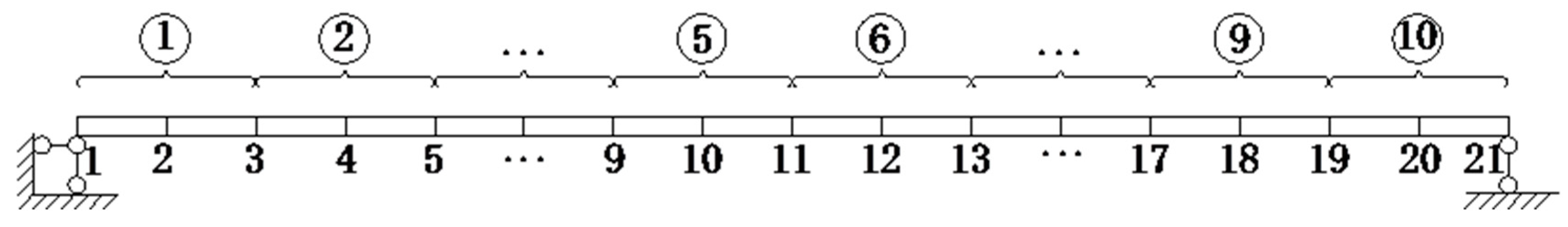
A simply supported steel beam was used as the experimental model. The elastic modulus and density of the steel were 210 GPa and , respectively. The section width, height, and span of the beam were 500 mm, 80 mm, and 1 m, respectively. The structure was divided into 10 substructures, each of which was divided into two units, consisting of a total of 20 units. The finite element model is shown in Figure 1. There were multiple damage cases, indicating 70%, 80%, and 60% residual stiffness in substructures 3, 5, and 8, respectively.
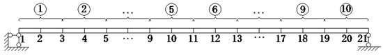
Figure 1.
Model of simply supported steel beam.
4.1.2. Virtual Mass Addition and Response Construction
According to the theory of the additional virtual mass method, first, the position of the additional virtual mass at the substructural midpoint is typically determined. Second, the optimal additional virtual mass is selected using the calculated relative sensitivity of the structural lower-order frequencies. Consider the addition of a virtual mass to substructure 5 as an example. The relative sensitivity of the first fourth-order frequency when the substructure 5 added with each 0.1 kg virtual mass was calculated (Figure 2). Based on the relative sensitivity calculations for the first fourth-order frequencies of each substructure with respect to the additional virtual mass value, 0.3 kg virtual mass was added to each substructure of the original structure to obtain ten different virtual structures.
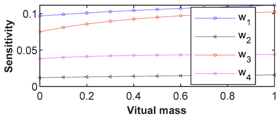
Figure 2.
Relative sensitivity of first fourth-order frequencies with virtual mass in substructure 5.
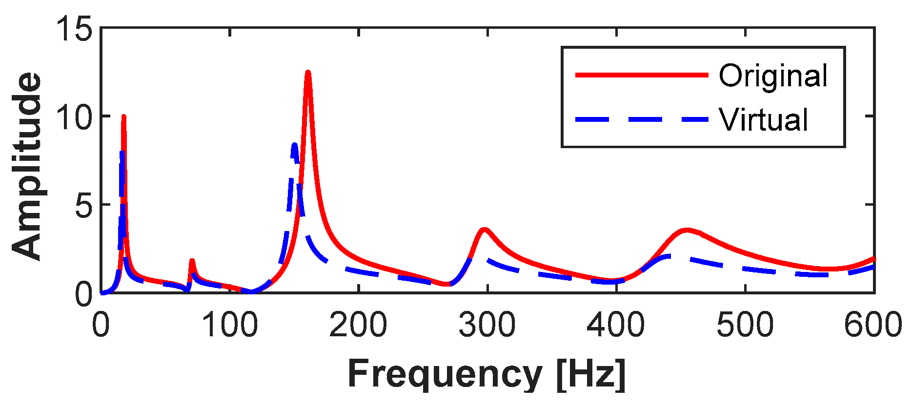
Impulse excitation was applied to the original structure with an action time of 2 s and a sampling frequency of 10,000 Hz to determine the acceleration response of the original structure and virtual structures. The acceleration response signal was preprocessed using an exponential window function. Based on Equation (2), the frequency-domain responses of the original and virtual structures, adding a virtual mass on substructure 5, were determined (Figure 3).
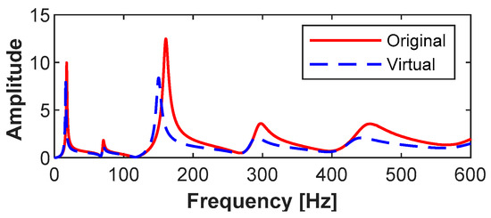
Figure 3.
Frequency-domain responses of original and virtual structures.
4.1.3. Damage Identification
The assumed damage factors of substructures 3, 5, and 8 were 70%, 80%, and 60%, respectively. The OMP method, Lasso regression model with the norm, and ridge regression model with the norm, which are three traditional damage identification methods based on sparsity, and the proposed IOMP method, were combined with the additional virtual quality method to identify each damage substructure and determine the degree of damage.
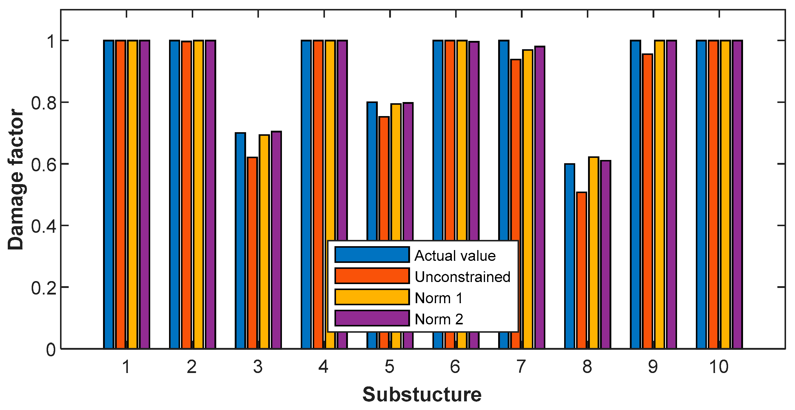
As shown in Figure 4, the damage recognition results for the objective function without sparse constraints showed damage to substructures 3, 5, 7, 8, and 9, indicating inconsistency with the actual local damage. When the regularization coefficient was 0.1 [28], the Lasso regression model with the norm and the ridge regression model with the norm could locate the damage positions more accurately. Under the norm constraint, the damage factors to substructures 3, 5, and 8 were 69.3%, 79.4%, and 62.2%, respectively, while substructure 7 is misjudged with 96.9% damage. Under the norm constraint, 70.4%, 79.7%, and 60.9% damage factors were identified in substructures 3, 5, and 8, respectively, while substructures 6 and 7 are misjudged as 99.6% and 98.1% damage, respectively. Both methods showed damage misjudgment, which directly resulted in larger deviations in identifying the degree of actual adjacent damage to the substructures. Nevertheless, the results significantly improved compared to the results for cases without constraint.
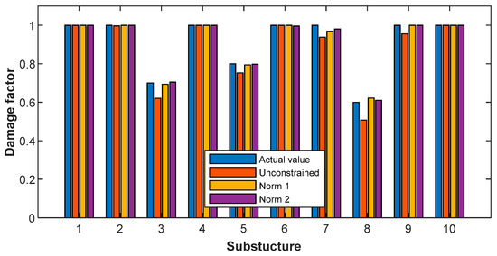
Figure 4.
Identification results of Lasso regression model with norm and ridge regression model with norm.
The damage identification results for the OMP method were relatively ideal from Figure 5. The damage extent identification of damaged substructures 3, 5, and 8 were 77.5%, 79.4%, and 55.6%, respectively, reflecting the actual damage conditions, but the damage to substructure 2 was misjudged. The corresponding identification values, 78.4%, 79.2%, and 54.9%, obtained using the IOMP method based on the residual variance criterion were relatively accurate, and no misjudgment of the undamaged substructures was observed.
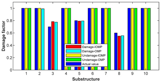
Figure 5.
Identification results obtained using OMP and IOMP method (residual variance criterion).
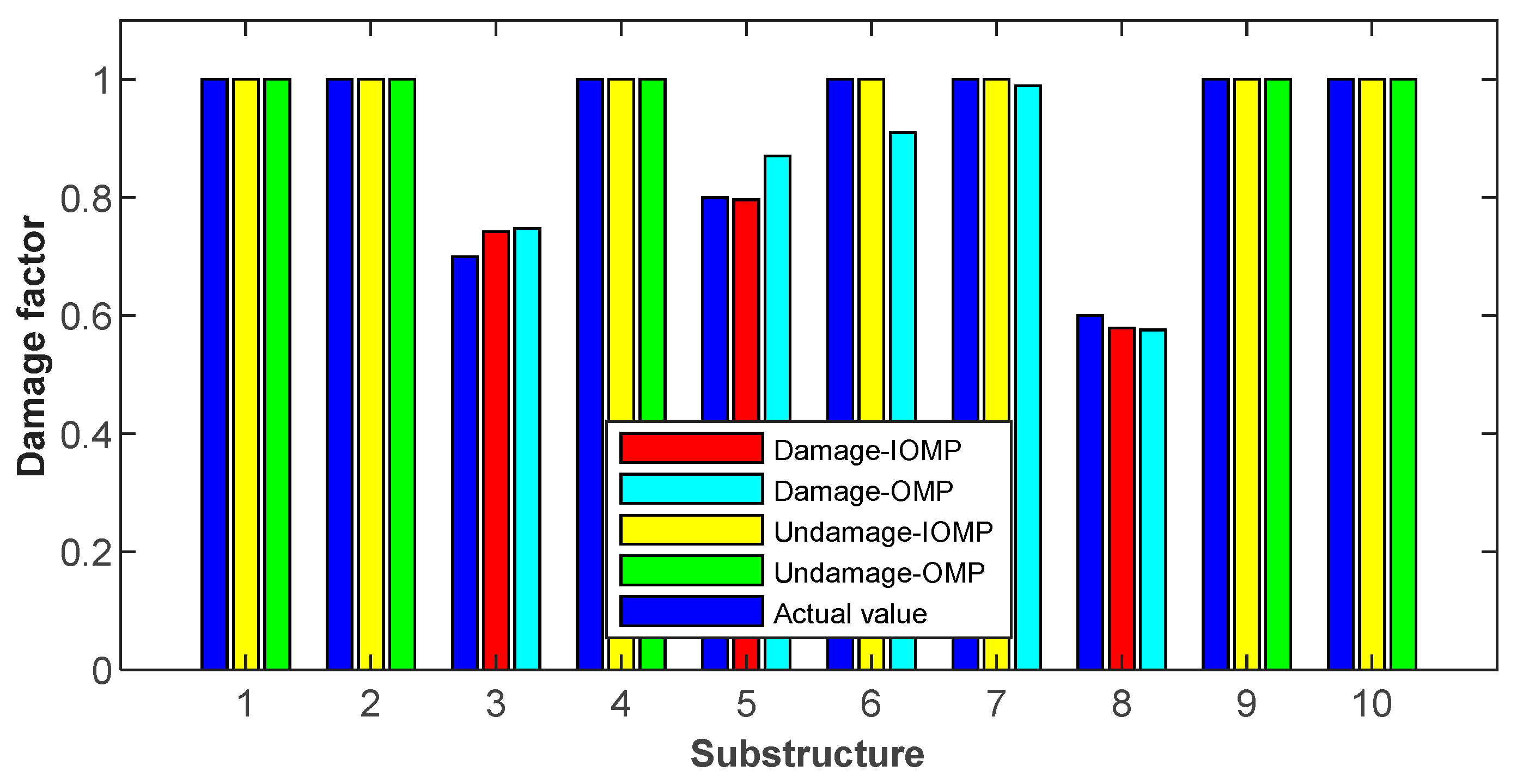
As shown in Figure 6, the OMP method misjudged the damage for substructures 6, and there was a significant difference in the identification between damage factors of actually damaged substructures and that of the IOMP method based on the sensitivity correlation criterion. The IOMP method based on the sensitivity correlation criterion showed 72.3%, 80.1%, and 59.0% damage factors recognition for substructures 3, 5, and 8, respectively. The identification accuracy satisfied the requirements, and no misjudgment of the undamaged substructures was observed.

Figure 6.
Identification results obtained using OMP and IOMP method (sensitivity correlation criterion).
As shown in Figure 7, when the regression model is non-parameter Gaussian kernel regression, the IOMP method is more accurate than OMP method. Because the non-parameter regression model is approximate, its accuracy is worse than the FEM model. However, the damaged substructures-selected process of the IOMP method has stronger integrality.

Figure 7.
Identification results obtained using OMP and IOMP method (Gaussian kernel regression model).
Both the OMP and IOMP methods determined the location and number of damaged substructures, and it was assumed that the remaining substructures were undamaged. The damage identification results indicated significant sparseness, consistent with the local damage conditions of actual structures. The residual vector () norms were compared to establish the superiority of the two methods, where k is the number of damaged substructures.
Under multiple damage conditions, the residual vector norm was large when the number of identified damaged substructures was one. The curve in Figure 8 starts when the number of damaged substructures is two to improve the image contrast. Damage residuals norm of the IOMP method based on the residual variance criterion and the IOMP method based on the sensitivity correlation criterion were lower than those of the OMP method, and the decrease rate was sharper. When the residual vector norm decreased to less than 0.025, the number of damaged substructures identified using the IOMP method was three, but that identified using the OMP method exceeded three. Therefore, the IOMP method yielded more accurate identification results than the OMP method, regardless of the degree of damage and the number of damaged substructures.

Figure 8.
Contrast with sparsity in simply supported beam simulation.
For researching the effect of considering nonlinearity, the results based on procedure expressed in Equation (18) are shown in Table 1.

Table 1.
Identification results of OMP and IOMP(S) method with nonlinearity iteration.
As shown in Table 1, neither OMP nor IOMP(S) have accurate results, which is most probably because of that the optimization in iteration of Equation (18) is not sparse. What is more important is the efficiency with nonlinearity iteration is much lower than without it.
4.1.4. Susceptibility to Noise
As mentioned in Section 4.1.1, the damaged substructures are the 3rd, 5th, and 8th, and both the methods could select the damaged substructures. So, the stability of the IOMP method to noise is verified by comparing the order and identification results of damaged substructures under different level noise. The order and identification result of selected damaged substructures with the IOMP method based on the residual variance criterion is almost same as that one of the sensitivity correlation criterion. Therefore, taking IOMP(S) as representative. The various noise level is 5%, 10%, 20%, and 30% rms. The results are shown in Table 2.
Table 2.
The order and identification result of selected damaged substructures under different level noise.
As known from Table 2, the identification results and selected order of damaged substructures are worse with noise increasing and that one of IOMP(S) is always better than OMP, which confirms that the susceptibility to noise of the IOMP methods is better. When the noise is in low level like 5% rms, the OMP method is accurate. However, the IOMP method has good results even in the noise level of 30% rms.
4.2. Space Truss Model
4.2.1. Model and Damage Scenario
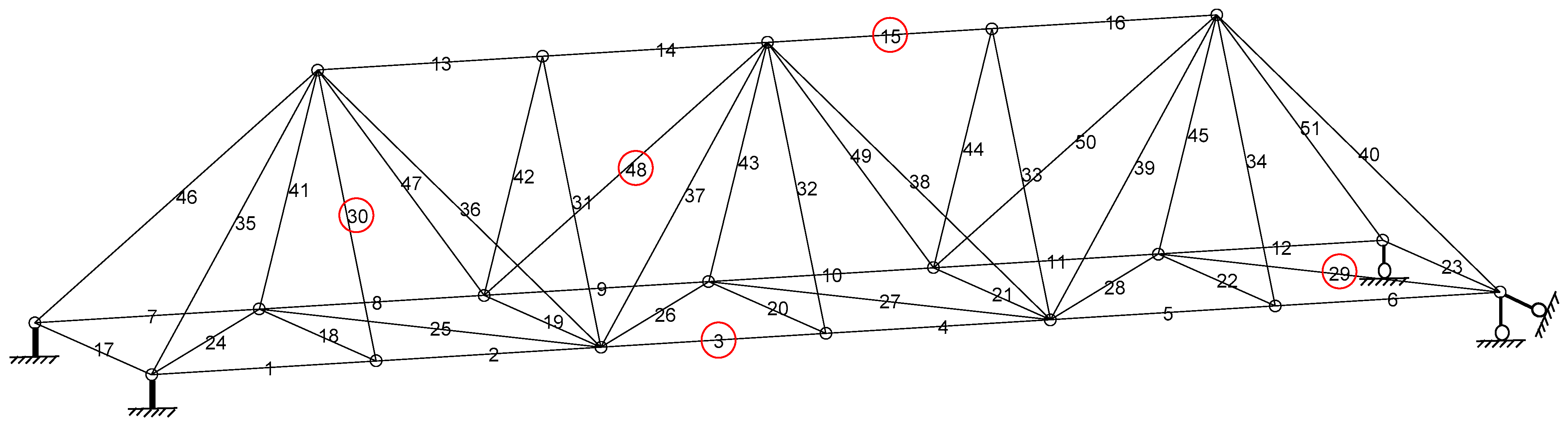
The size of this space truss model is , and the bars are articulated between each other. This model consists of 51 bars. Each bar is a hollow pipe, in which the outer diameter is 1 cm and thickness is 3 mm. The position and number of bars are shown in Figure 9. The elastic modulus, density, and position ratio of structural material were 206 GPa, , and 0.3, respectively. The damage scenario is assumed that the 3rd, 15th, 29th, 30th, and 48th bars respectively contain 50%, 70%, 60%, 77%, and 82% residual stiffness. And the position of damaged bars have been marked with read circle in Figure 9.
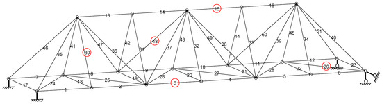
Figure 9.
Space truss and bars number.
4.2.2. Damage Identification
In this section, considering the complexity of the space truss, the non-parameter Gaussian kernel regression model is adopted. The first frequency of the 51 virtual structures under real damage situation, which is constructed by respectively adding 1.2 kg virtual mass on each bar, is chosen to optimize the damage factors. The results of OMP and IOMP method are shown in Table 3.
Table 3.
Identification results of space truss by OMP and IOMP method.
As known from Table 3, the identification results of IOMP method is more accurate than OMP method. Either the selected damaged substructures or the residual stiffness of OMP method has more error, which might be caused by the complexity of space truss or the non-parameter regression model.
5. Verification of Frame Experiment
5.1. Model and Damage Scenario
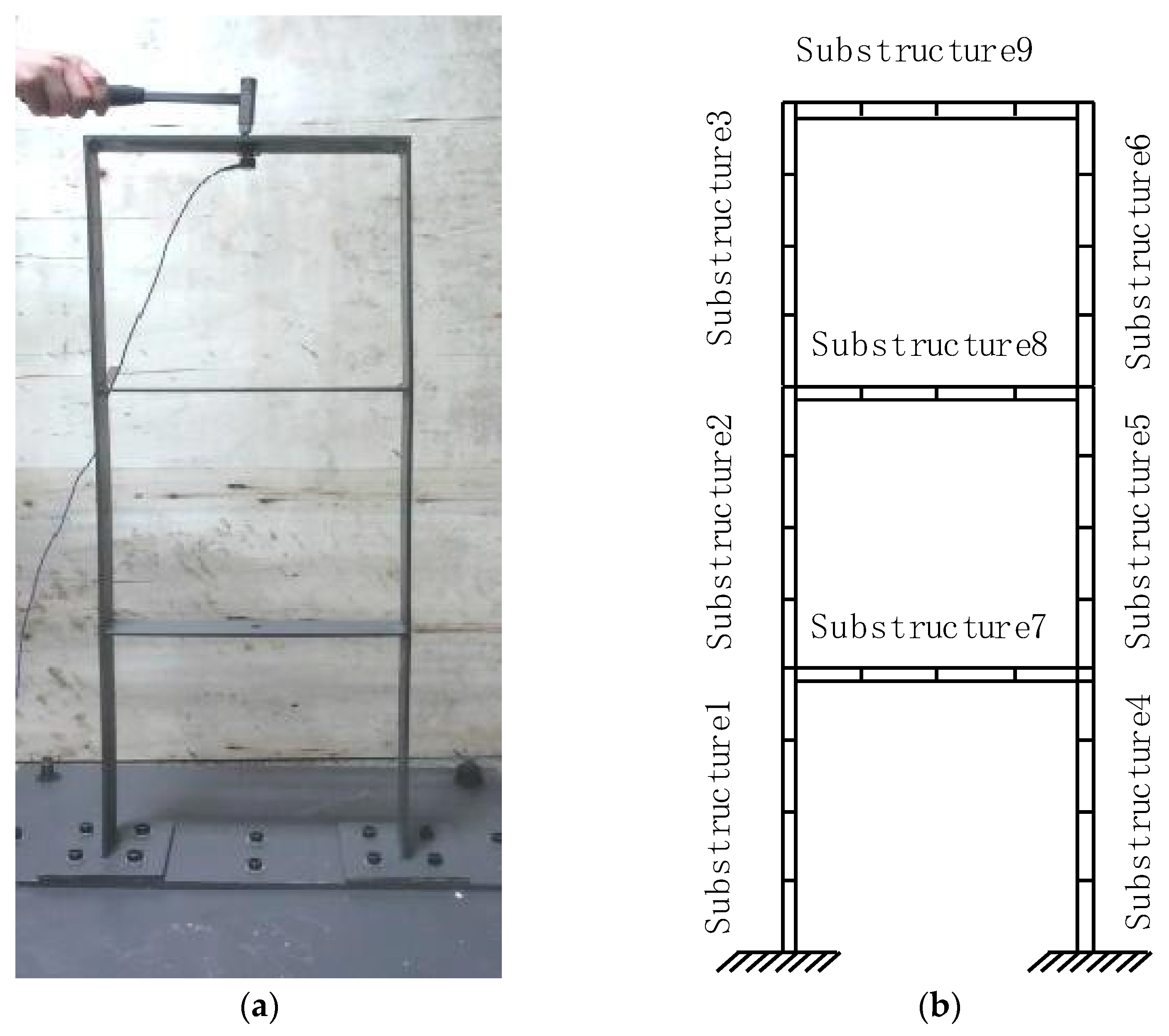
The experimental three-layer plane frame structure was made of Q235 steel, shown in Figure 10a. Its elastic modulus was 2.10 GPa, and its density was . The height and span of each layer were identical, which is 0.3 m. The cross-section dimension is . The frame contained nine substructures and 36 elements, with each substructure having four units. The finite element model is shown in Figure 10b.
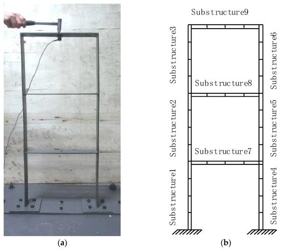
Figure 10.
Frame model. (a) experimental picture; (b) FEM.
The experimental frame model damage was achieved by producing a 1 cm deep, 1 mm wide, and 1 cm spacing incision on substructure 2. Under this condition, the stiffness of substructure 2 decreased by 33%, indicating that the damage factor was 0.67. In addition, an incision of 1.5 cm depth, 1 mm width, and 1 cm spacing was made on substructure 9. Its stiffness decreased by 50%, showing that the damage factor was 0.5. During the experimental tests, the load and structural acceleration responses were measured. The required equipment included a modal force hammer, acceleration sensor, and data acquisition instrument.
5.2. Framework Dynamic Testing and Response Construction with Additional Virtual Mass
- Dynamic testing of undamaged structure: An acceleration sensor was installed in the middle position of substructures, and the other side was hit with a modal force hammer several times to obtain multiple sets of loads and acceleration response data. The measured data were processed to determine the experimental frequencies of the undamaged structures.
- Dynamic testing of damaged structure: The sensor was installed in the middle position of the substructures, and the structure was hit with a modal force hammer on the other side to obtain multiple sets of loads and acceleration data.
The acceleration response data of the virtual structure was constructed using the additional virtual mass method, and the structure frequency was identified according to the Eigen system realization achievement method. The virtual structure formed after the virtual mass was added to the ith substructure and is denoted as. The average values of the fourth-order frequency of the 9 virtual structures are listed in Table 4.
Table 4.
Selected fourth-order frequency means (Hz).
5.3. Damage Identification
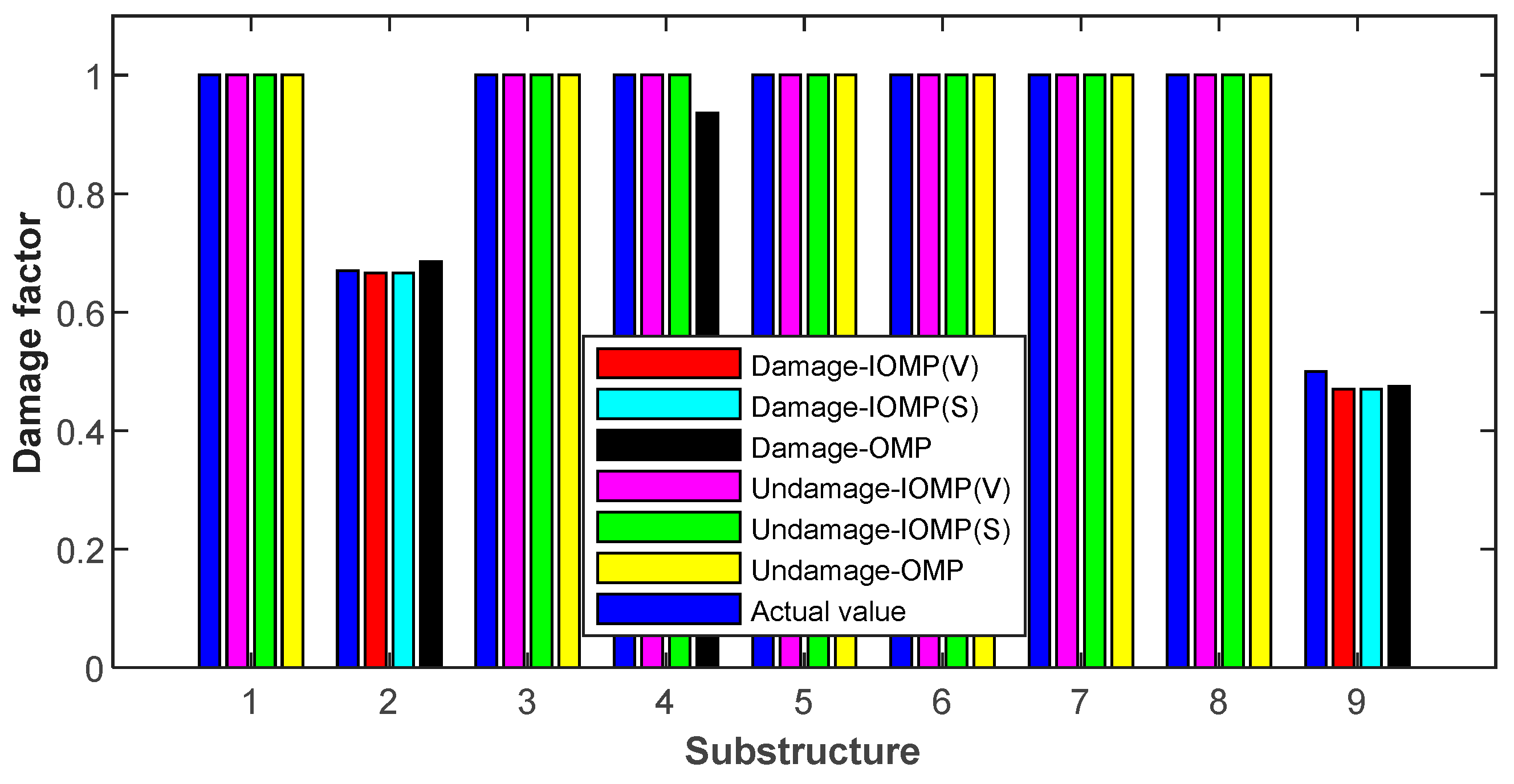
Based on the experimental frequency values of the damage structures, the OMP method and the two types of IOMP methods were used for damage identification. The identification results were as follows: substructures 2 and 9 were actual damaged, and the damage factors were 0.67 and 0.5, respectively.
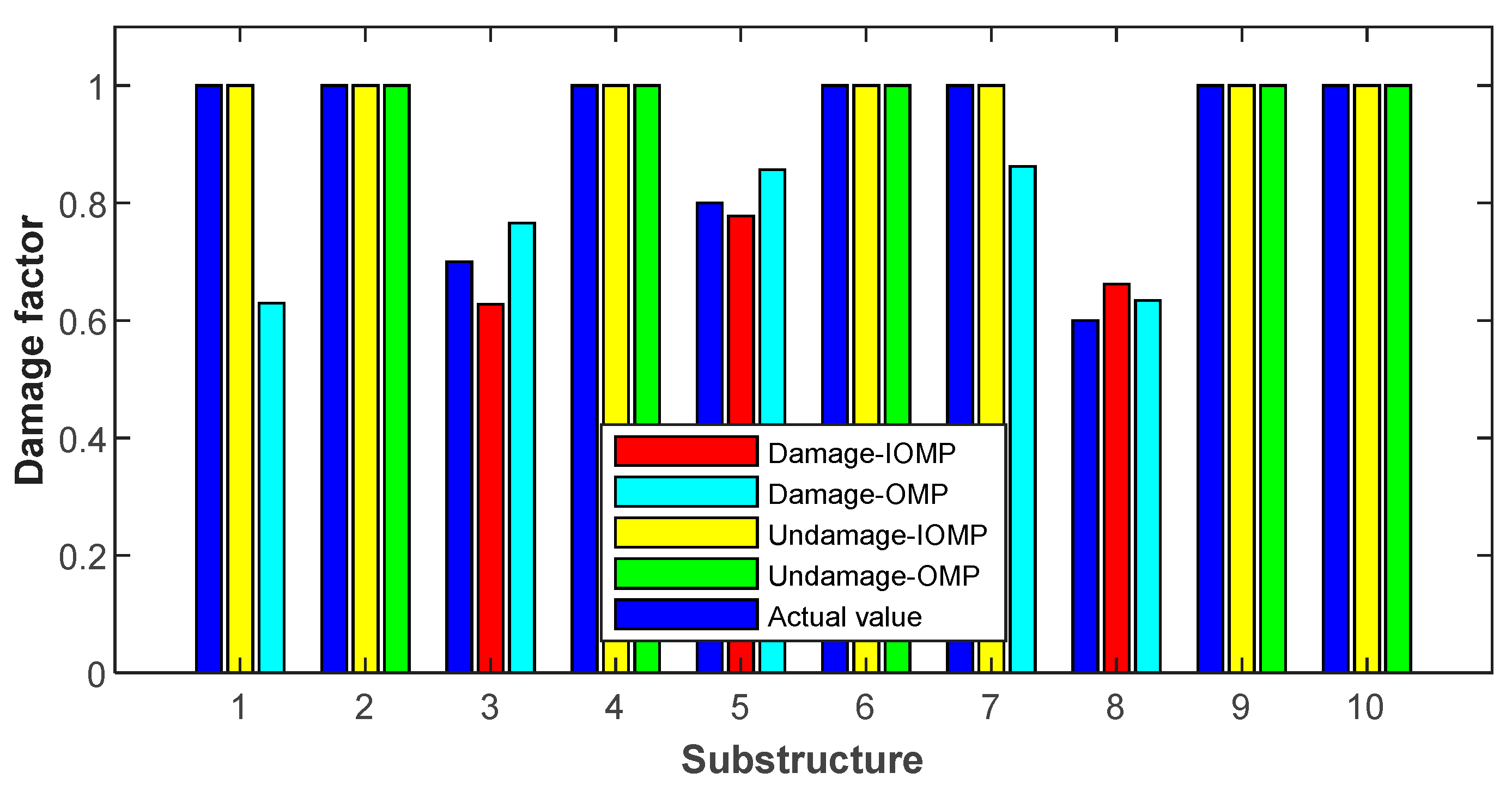
The damage factors obtained using the three methods are listed in Table 5. The damage factors of substructures 2 and 9 identified using the OMP method were 0.685 and 0.475, respectively, close to the actual damage (Figure 11). These results indicated that the OMP method exhibited high accuracy in damage identification but misjudged the undamaged substructure 4. The damage factor identification values based on the two IOMP methods for damage substructures 2 and 9 were 0.666 and 0.47, respectively, consistent with the actual damage results. These findings show that the IOMP damage identification method based on additional virtual mass can precisely identify the damage to this frame model.
Table 5.
Damage factors identification values obtained using OMP and IOMP method.
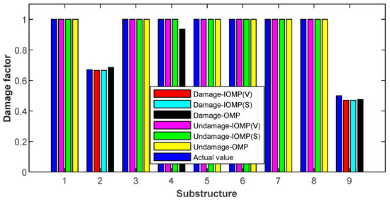
Figure 11.
Damage identification results.
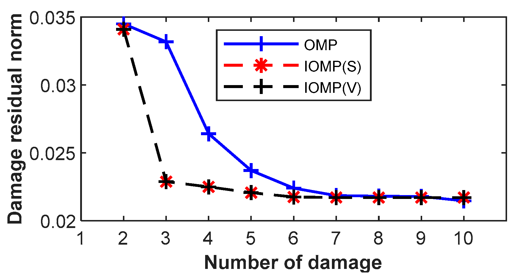
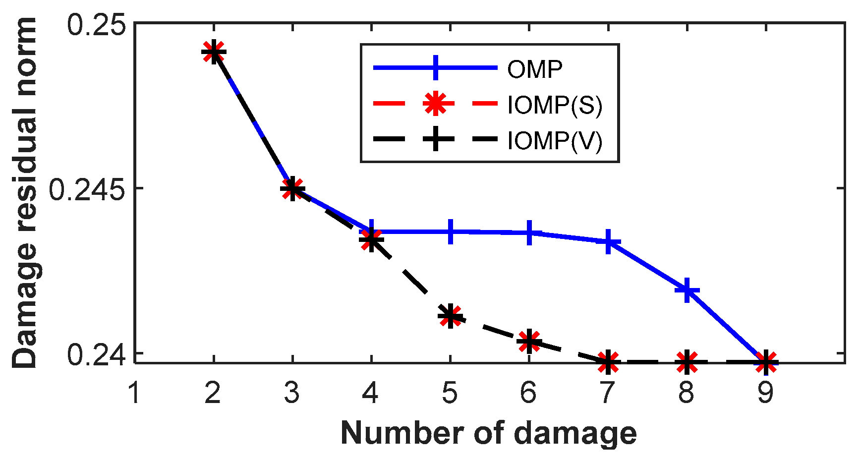
When the OMP and IOMP methods were used for damage identification, it was necessary to determine the number of substructures preliminarily that could be damaged. After calculations, a broken line chart of the damage residual norm with the number of damaged substructures was plotted in Figure 12. When the number of damaged substructures was two, the damage residual norm was approximately 0.249. Because of the high accuracy of the experimental data, the OMP and IOMP methods both showed good performance in determining the number of damaged substructures. However, when the number of identified damage substructures were equal, the residual norm of the IOMP method was always smaller than that of the OMP method, indicating that the IOMP method was more accurate than the OMP method.

Figure 12.
Contrast with sparsity in frame Experiment.
6. Conclusions
In this study, an IOMP method combined with the additional virtual mass was developed to improve damage identification based on structural modal and minimize susceptibility to structural modal data, measurement point distribution, and noise, considering the initial condition of sparse structural damage. Through numerical simulation of a simply supported steel beam and the experimental verification of the steel frame model, the following conclusions are drawn:
- The IOMP method combined with the additional virtual mass method can effectively expand structural modal information to improve the accuracy of structural damage identification while constraining the optimization results to obtain sparse optimization results consistent with the actual local damage.
- Compared to the Lasso regression model with the norm and the ridge regression model with the norm, the IOMP method selects independently damage substructures, which satisfies the initial condition that structural damage is sparse. In addition, the IOMP method does not need to select the regularization coefficient , and thus, eliminates its direct influence on the optimization results to obtain more accurate damage identification results.
- The IOMP method improves the deficiency of the OMP method in that the recognition result is a local optimal solution when combined with the additional virtual mass method, which integrates the recognition result better. Furthermore, it improves the logical defects of the OMP method effectively in predicting damage sparsity. The IOMP method is also accurate for selecting damaged substructures.
Author Contributions
Conceptualization, Q.Z. and J.H.; methodology, D.X. and H.W.; software, D.X. and J.H.; validation, Q.Z. and Ł.J.; formal analysis, Q.Z. and D.X.; resources, J.H.; writing—original draft preparation, Q.Z. and D.X.; writing—review and editing, J.H. and Ł.J.; visualization, H.W.; supervision, Q.Z.; funding acquisition, J.H. All authors have read and agreed to the published version of the manuscript.
Funding
This research was funded by National Natural Science Foundation of China (NSFC) (51878118), of the Educational Department of Liaoning Province (LJKZ0031), of the Liaoning Provincial Natural Science Foundation of China (20180551205), of the Fundamental Research Funds for the Central Universities (DUT19LK11), and of the National Science Centre, Poland (project 2018/31/B/ST8/03152).
Institutional Review Board Statement
Not applicable.
Informed Consent Statement
Not applicable.
Data Availability Statement
The data presented in this study are available on request from the corresponding author.
Conflicts of Interest
The authors declare no conflict of interest.
References
- Toh, G.; Park, J. Review of Vibration-Based Structural Health Monitoring Using Deep Learning. Appl. Sci. 2020, 10, 1680. [Google Scholar] [CrossRef]
- Annamdas, V.G.M.; Bhalla, S.; Soh, C.K. Applications of structural health monitoring technology in Asia. Struct. Health Monit. 2017, 16, 324–346. [Google Scholar] [CrossRef]
- Hou, J.L.; Wang, S.J.; Zhang, Q.X.; Jankowski, L. An Improved Objective Function for Modal-Based Damage Identification Using Substructural Virtual Distortion Method. Appl. Sci. 2019, 9, 971. [Google Scholar] [CrossRef] [Green Version]
- Fan, W.; Qiao, P.Z. Vibration-based Damage Identification Methods: A Review and Comparative Study. Struct. Health Monit. 2011, 10, 83–111. [Google Scholar] [CrossRef]
- Seo, J.; Hu, J.W.; Lee, J. Summary Review of Structural Health Monitoring Applications for Highway Bridges. J. Perform. Constr. Facil. 2016, 30, 9. [Google Scholar] [CrossRef]
- Weng, S.; Zhu, H.P.; Xia, Y.; Li, J.J.; Tian, W. A review on dynamic substructuring methods for model updating and damage detection of large-scale structures. Adv. Struct. Eng. 2020, 23, 584–600. [Google Scholar] [CrossRef]
- Cao, M.S.; Ding, Y.J.; Ren, W.X.; Wang, Q.; Ragulskis, M.; Ding, Z.C. HierarchicalWavelet-Aided Neural Intelligent Identification of Structural Damage in Noisy Conditions. Appl. Sci. 2017, 7, 391. [Google Scholar] [CrossRef] [Green Version]
- Chang, M.; Kim, J.K.; Lee, J. Hierarchical neural network for damage detection using modal parameters. Struct. Eng. Mech. 2019, 70, 457–466. [Google Scholar]
- Maia, N.M.M.; Silva, J.M.M.; Almas, E.A.M.; Sampaio, R.P.C. Damage detection in structures: From mode shape to frequency response function methods. Mech. Syst. Signal Proc. 2003, 17, 489–498. [Google Scholar] [CrossRef]
- Huang, Q.; Xu, Y.L.; Li, J.C.; Su, Z.Q.; Liu, H.J. Structural damage detection of controlled building structures using frequency response functions. J. Sound Vib. 2012, 331, 3476–3492. [Google Scholar] [CrossRef]
- Xie, L.Y.; Zhou, Z.W.; Zhao, L.; Wan, C.F.; Tang, H.S.; Xue, S.T. Parameter Identification for Structural Health Monitoring with Extended Kalman Filter Considering Integration and Noise Effect. Appl. Sci. 2018, 8, 2480. [Google Scholar] [CrossRef] [Green Version]
- Shi, Z.Y.; Law, S.S.; Zhang, L.M. Damage localization by directly using incomplete mode shapes. J. Eng. Mech. ASCE 2000, 126, 656–660. [Google Scholar] [CrossRef]
- Sinha, U.; Chakraborty, S. Detection of Damages in Structures Using Changes in Stiffness and Damping. In Recent Advances in Computational Mechanics and Simulations; Volume-I: Materials to Structures.Lecture Notes in Civil Engineering (LNCE 103); Springer: Singapore, 2021; pp. 259–271. [Google Scholar]
- Rao, P.S.; Ramakrishna, V.; Mahendra, N.V.D. Experimental and Analytical Modal Analysis of Cantilever Beam for Vibration Based Damage Identification Using Artificial Neural Network. J. Test. Eval. 2018, 46, 656–665. [Google Scholar] [CrossRef]
- Ali, J.; Bandyopadhyay, D. Experimental validation of the proposed technique for condition monitoring of structure using limited noisy modal data. Int. J. Struct. Integr. 2020, 11, 45–59. [Google Scholar] [CrossRef]
- Wu, Q.; Guo, S.; Li, X.; Gao, G. Crack diagnosis method for a cantilevered beam structure based on modal parameters. Meas. Sci. Technol. 2020, 31, 035001. [Google Scholar] [CrossRef]
- Chang, K.-C.; Kim, C.-W. Modal-parameter identification and vibration-based damage detection of a damaged steel truss bridge. Eng. Struct. 2016, 122, 156–173. [Google Scholar] [CrossRef]
- Bhowmik, B.; Tripura, T.; Hazra, B.; Pakrashi, V. Real time structural modal identification using recursive canonical correlation analysis and application towards online structural damage detection. J. Sound Vib. 2020, 468, 115101. [Google Scholar] [CrossRef]
- Ghahremani, B.; Bitaraf, M.; Rahami, H. A fast-convergent approach for damage assessment using CMA-ES optimization algorithm and modal parameters. J. Civ. Struct. Health Monit. 2020, 10, 497–511. [Google Scholar] [CrossRef]
- Rainieri, C.; Gargaro, D.; Reynders, E.; Fabbrocino, G. A study on the concurrent influence of liquid content and damage on the dynamic properties of a tank for the development of a modal-based SHM system. J. Civ. Struct. Health Monit. 2020, 10, 57–68. [Google Scholar] [CrossRef]
- Dinh, H.M.; Nagayama, T.; Fujino, Y. Structural parameter identification by use of additional known masses and its experimental application. Struct. Control Health Monit. 2012, 19, 436–450. [Google Scholar] [CrossRef]
- Rajendran, P.; Srinivasan, S.M. Performance of rotational mode based indices in identification of added mass in beams. Struct. Eng. Mech. 2015, 54, 711–723. [Google Scholar] [CrossRef]
- Dems, K.; Mroz, Z. Damage identification using modal, static and thermographic analysis with additional control parameters. Comput. Struct. 2010, 88, 1254–1264. [Google Scholar] [CrossRef]
- Hou, J.L.; Jankowski, L.; Ou, J.P. Structural damage identification by adding virtual masses. Struct. Multidiscip. Optim. 2013, 48, 59–72. [Google Scholar] [CrossRef]
- Knitter-Piatkowska, A.; Dobrzycki, A. Application of Wavelet Transform to Damage Identification in the Steel Structure Elements. Appl. Sci. 2020, 10, 8198. [Google Scholar] [CrossRef]
- Wang, S.; Xu, M.; Xia, Z.; Li, Y. A novel Tikhonov regularization-based iterative method for structural damage identification of offshore platforms. J. Mar. Sci. Technol. 2019, 24, 575–592. [Google Scholar] [CrossRef]
- Wu, Y.-H.; Zhou, X.-Q. L-1 Regularized Model Updating for Structural Damage Detection. Int. J. Struct. Stab. Dyn. 2018, 18, 1850157. [Google Scholar] [CrossRef]
- Weber, B.; Paultre, P. Damage Identification in a Truss Tower by Regularized Model Updating. J. Struct. Eng. 2010, 136, 307–316. [Google Scholar] [CrossRef]
- Hou, R.; Xia, Y.; Bao, Y.; Zhou, X. Selection of regularization parameter for l(1)-regularized damage detection. J. Sound Vib. 2018, 423, 141–160. [Google Scholar] [CrossRef]
- Racine, J.S. Foundations and Trends: Nonparametric Econometrics: A primer; Now Publishers Inc.: Boston, MA, USA, 2008; Volume 3, pp. 1–88. [Google Scholar]
- Dhulipala, S.J.S. Gaussian Kernel Methods for Seismic Fragility and Risk Assessment of Mid-Rise Buildings. Sustainability 2021, 13, 2973. [Google Scholar] [CrossRef]


Publisher’s Note: MDPI stays neutral with regard to jurisdictional claims in published maps and institutional affiliations. |
© 2021 by the authors. Licensee MDPI, Basel, Switzerland. This article is an open access article distributed under the terms and conditions of the Creative Commons Attribution (CC BY) license (https://creativecommons.org/licenses/by/4.0/).