Abstract
When the finite element-strength reduction method is used for two-dimensional slope stability analysis for elastic-perfectly plastic material, the failure criterion usually adopts the criterion of plastic zone penetration. That is, when the slope is in the limit equilibrium state, the plastic zone goes through the slope from the toe to the top. Meanwhile, the critical slip surface is composed of a series of points of maximum equivalent plastic strain along the depth direction. By deploying a set of parallel lines approximately perpendicular to the slope surface and picking out the points of these lines with the maximum equivalent strain points, we obtain a series of points taking on a wave shape, which constitutes a signal function. Subsequently, the wavelet packet analysis is used to smooth these points, i.e., locating the critical slip surface. The analysis of classic examples and comparison with Spencer’s method show that the proposed method in this paper is reasonable and effective.
1. Introduction
The finite element method is the most widely used method for slope stability analysis (SSA). Its strong ability in nonlinear analysis gives the finite element method (FEM) great potential in geotechnical engineering. It was first introduced to geotechnical engineering by Clough and Woodward [1]. In SSA, the factor of safety (FOS) is defined as the ratio of the actual soil shear strength to the minimum shear strength required to prevent failure [2]. As Duncan [3] pointed out, the FOS is the factor that continuously reduces the soil shear strength to bring the slope to the verge of failure. This method, which brings slope into a limit equilibrium state (LES) by reducing the shear strength of the soil, is called the strength reduction method (SRM), was first used in SSA by Zienkiewicz et al. [4], and has been studied by Naylor [5], Wong [6], Donald et al. [7], Matsui et al. [8], Duncan, and others. Griffiths et al. systematically summarized the advantages of the finite element method–strength reduction method compared with limit equilibrium methods (LEM) [9] in SSA; more detail can be found in [10].
In the past few decades, various other effective numerical methods have also been developed for SSA, such as the mesh-free methods [11], the virtual element method [12], the boundary element method [13,14], the smoothed particle hydrodynamics [15], the material point method [16,17], the discrete element method [18], the numerical manifold method [19] and other numerical methods [20,21]. Great progress also has been made in the research of three-dimensional SSA [22,23,24,25,26,27,28], but two-dimensional SSA is still a hot academic issue [12,29,30,31,32,33,34,35,36,37].
In practice, there are two crucial issues in the SSA: calculation of the FOS and location of the critical slip surface (CSS). However, research into SRM is mainly concentrated on the computation of the FOS rather than locating the CSS. By bringing the slope to LES, the FOS agreeing with the LEM can be easily obtained. In contrast, the CSS of a slope is usually determined approximately through visualization techniques, such as the distribution of maximum shear-strain rates [4], shear-strain increment distributions [8], yielding regions of the slope [38], the velocity field at collapse [39], or other technical measures. However, to this day, there is no rigorous mathematical method to locate the CSS.
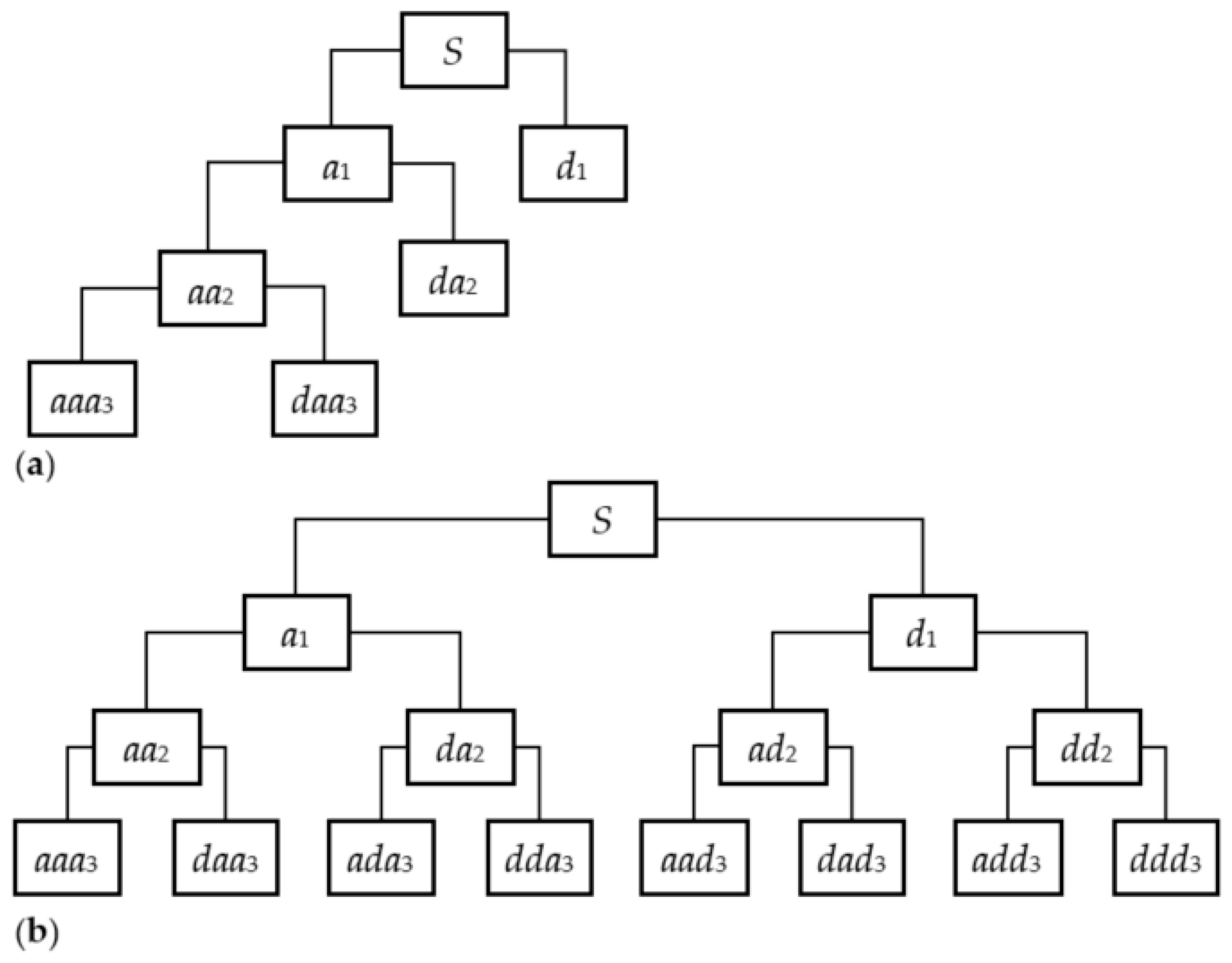
For two-dimensional SSA, Zheng et al. [40] developed a new approach to search the CSS for any yield criterion by using the equivalent plastic strain field in the LES, in which the least-square method is used to fit the CSS. However, for a complicated slope composed of multiple materials, its CSS shape may contain several turning points [41], and the least-square method will not be applicable in this case. For this reason, the wavelet method [42] was proposed and applied to the analysis of homogeneous and multi-layer slopes, in which the maximum equivalent plastic strain point is regarded as a signal function, and the high-frequency part of the signal is filtered to obtain a smooth CSS. The results show that the wavelet method has good applicability. Wavelet analysis is a rapidly developing new field in applied mathematics and engineering [43]. It can be used for damage detection [44], time-frequency analysis [45], signal-to-noise separation [46], multi-scale edge detection [47], and so on. Wavelet packet analysis (WPA) divides the time-frequency more carefully, and its resolution of the high-frequency part of the signal is higher than that of the dyadic wavelet. In other words, the dyadic wavelet only further decomposes the low-frequency part into low-frequency and high-frequency parts, while wavelet packet decomposition further decomposes both low-frequency and high-frequency parts as shown in Figure 1. Hence, the wavelet packet has a wide range of application values [48]. The application of new mathematical methods for the solution of engineering problems can not only introduce the methods but also shorten the distance between the methods and applications.

Figure 1.
Three-layer decomposition. (a) Wavelet; (b) Wavelet packet.
In this study, the SRM and the WPA are combined for the SSA. As in [42], the distribution of maximum equivalent plastic strain points in this study is regarded as a signal function, which is filtered by wavelet packet denoising technology to obtain a smooth CSS. The implementation step is as follows: First, the SRM is used to bring the slope into the LES and calculate the FOS. Second, deploying a series of parallel lines approximately perpendicular to the slope surface, and picking out the points of these lines with the maximum equivalent plastic strain points, is noted as yi (xi). Third, the wavelet packet filter is used to smooth yi (xi) and the location of the CSS is accordingly determined. Three numerical examples including a homogeneous slope, a slope containing a weak intercalated layer, and a soil–rock mixture slope are employed to validate the proposed method.
2. Slope Stability Analysis by the SRM
For SRM, there may be a significant difference in the failure loads or FOS if different failure criteria are selected [49]. At present, there are several common failure criteria: (1) non-convergence of the numerical solution [10,38,50]; (2) a sudden increase in the deformation of a characteristic location [51]; (3) connectivity of the shear increment strain or shear-strain region [8]. Since many factors may lead to the non-convergence of this numerical calculation, non-convergence does not necessarily mean the failure of the structure, thus the first criterion is considered insufficient. For the second criterion, this method needs to constantly draw the displacement–reduction factor curve to judge the position of the turning point through observation, so this criterion is also considered not objective enough.
For an elastic-perfectly plastic model with an associated flow rule, when a point within the slope is in the plastic state, Zheng et al. [52] proved that the elastoplastic matrix Dep at that point must be a positive semidefinite matrix with a rank defect of one and found out the direction of the singularity of Dep. Based on this fact, Zheng suggested that the failure criterion of the slope should be considered the moment when the strip runs through from the toe to the top of the slope, and all the elements in the strip are in the plastic state. Therefore, the third criterion, i.e., plastic zone penetration, was chosen as the failure criterion in this study, and the assumptions are adopted too.
In practice, we take the reduction factor Fi corresponding to the LES as the FOS. Once the failure criterion is selected, the FOS and the distribution of the equivalent plastic strain (EPS) in the LES can be easily obtained by RSM. The EPS is defined as follows:
where is incremental plastic strain vector in a load; the sum is performed with all load steps.
In this paper, the failure criterion based on plastic zone penetration is adopted. Once a slope arrives at the LES, a contour line of with a small value, it passes through the slope from the toe to the top. The larger of a contour line, the larger the plastic deformation of the closed area of the contour line, and the more serious the slope damage is [41]. Therefore, it can be known that the CSS goes through the points at which the equivalent plastic strain obtains the maximum in the vertical direction. Due to the interpolation characters of the isoparametric elements, the maximizers will generally not be on a smooth curve but take the form of a wave. Based on this observation, a new method was proposed by Zheng et al. for searching the CSS.
3. Wavelet and Wavelet Packet Transformation and Reconstruction
3.1. Wavelet Transformation and Reconstruction
A wavelet is a special kind of function with oscillation and can quickly decay to zero, and tends to be irregular and asymmetric [53]. In general, the mother wavelet is restricted, and function should be governed as follows
where is Fourier transform of .
By the dilation and translation of , the wavelet basis can be defined as follows
where the parameter a > 0 indicates the scale factor and the parameter b∈R represents the displacement factor.
For the signal function , after wavelet decomposition, the coefficients are
where is the complex conjugate function of .
The inverse wavelet transform formula is
Defining , , and, the corresponding binary discrete wavelet function sequence can be formulated as
and when , the discrete wavelet transform is
3.2. Multi-Resolution Analysis
Mallat first proposed a multi-resolution analysis (MRA) and presented a fast algorithm based on wavelet transformation and reconstruction, named the Mallat algorithm. According to the Mallat algorithm, if contains the sampling information of , and , the orthogonal wavelet decomposition formula is
where is the scaling coefficients, is the wavelet coefficients, j is the layer of decomposition, and N is the sampling points.
In this, h and g are orthogonal filters generated by the scale function and wavelet function , respectively. These are defined as
The reconstruction procedure is an inverse transform of the decomposition. The reconstruction formula is
A wavelet has the property of multi-resolution, which can treat signal data in multi-resolution analysis and decompose a signal interwoven with different frequencies into different frequency sub-signals.
3.3. Wavelet Packet Transform and Reconstruct
In the MRA of signal function, the original signal is first decomposed into two parts, low frequency and high frequency, and then the low-frequency part is further decomposed into low frequency and high frequency, and then it is decomposed gradually. However, in wavelet packet decomposition (WPD), each scale is broken down into high frequency and low frequency simultaneously, so the resolution is higher.
The wavelet package can be created by scale function and wavelet function . The definition is as follows
where n is a wavelet packet parameter, h and g are orthogonal filters [54], , and .
Binary scaling and translation can also be performed for
For orthogonal wavelet packet analysis, the algorithm is very similar to the Mallat algorithm of orthogonal wavelet analysis. The following recursive formula can achieve the wavelet packet transform
where is the wavelet packet coefficient, defined by
The reconstruction wavelet packet procedure is an inverse transform of the decomposition. The reconstruct recursive equation is
The essentials of wavelet packet decomposition are to divide a signal into different frequency spans layer-by-layer. If the original signal contains enough information, the frequency span can be divided very subtly.
The equation deduces that if the decomposition layer is chosen appropriately, we can obtain the beginning and end of expected frequency spans—and with this method, the original signal when every frequency is wider enough [55]. Thus, there is no need to locate the frequency spans accurately for the ingredients which we needed so that it can adjust frequency drift.
The advantage of reconstruction is that we can choose all the frequency bins or some parts of them and set the others (noise or random interruption) as zero. Thus, if we can decompose a signal into different frequency bins, it is much easier to extract noise during the reconstruction. Figure 1 illustrates the three-layer wavelet and wavelet packet decomposition, where a represents the low-frequency part and d represents the high-frequency part.
According to the entropy standard, a set of orthogonal bases selected from the wavelet packet is called a wavelet packet basis of . Different wavelet packet bases result in different signal decomposition. The optimal wavelet tree can be selected according to the entropy standards [56]. Matlab software provides Shannon entropy, entropy threshold (threshold), norm entropy (norm), Sure entropy, log energy entropy (log energy), and user-defined entropy. Among these standards, Shannon entropy is used to select the optimal wavelet tree in this article.
3.4. Threshold Processing of Wavelet Packet Decomposition Coefficients
After selecting the optimal wavelet packet tree, we can use a threshold to remove the noise in wavelet packet nodes. There are many threshold denoising methods in practice. The commonly used threshold functions are soft threshold and hard threshold, and the calculation formulas are as follows:
Soft threshold:
Hard threshold:
Based on Matlab software, we can use the “ddencmp.m” function to obtain the default threshold value of the signal data. The methods to obtain these values include the soft and hard threshold methods. We can also use the “wpthcoef.m” function to deal with the threshold values of wavelet packet coefficients [57].
4. Searching the CSS Based on the Wavelet Packet
In finite element analysis, due to the interpolation characters of the isoparametric elements, yi (xi) is not on a smooth curve but in the form of a wave. Each line has only one maximum point, and these points constitute a set of good signal data yi (xi). Our task is to use a wavelet packet to smooth these points and locate the CSS.
The algorithm steps of the proposed method are as follows:
- (1)
- Combined with FEM, the SRM is used to bring the slope into the LES and obtain the FOS of the slope.
- (2)
- The coordinates of the maximum equivalent plastic strain point are sought in the plastic zone of the slope. Firstly, a set of parallel lines are arranged along the slope depth direction, then the corresponding search points are deployed on each line, and finally the coordinates of the maximum equivalent plastic strain point are searched by interpolation.
- (3)
- The obtained data points are decomposed by wavelet packet. According to the given signal data, a suitable wavelet basis function and the decomposition level is determined. Although there exist a huge number of possible wavelet bases, this paper is limited to the Daubechies orthogonal wavelet family. After the test, the Daubechies six-coefficient wavelets were used in all work.
- (4)
- The wavelet packet coefficients are processed by threshold quantization. According to the distribution of the data and its high-frequency part, each frequency band’s wavelet packet decomposition coefficients are processed by a threshold.
- (5)
- Wavelet packet reconstruction is performed. The processed wavelet packet decomposition coefficients are reconstructed by wavelet packet, and the location of the CSS is obtained by connecting the corresponding data points.
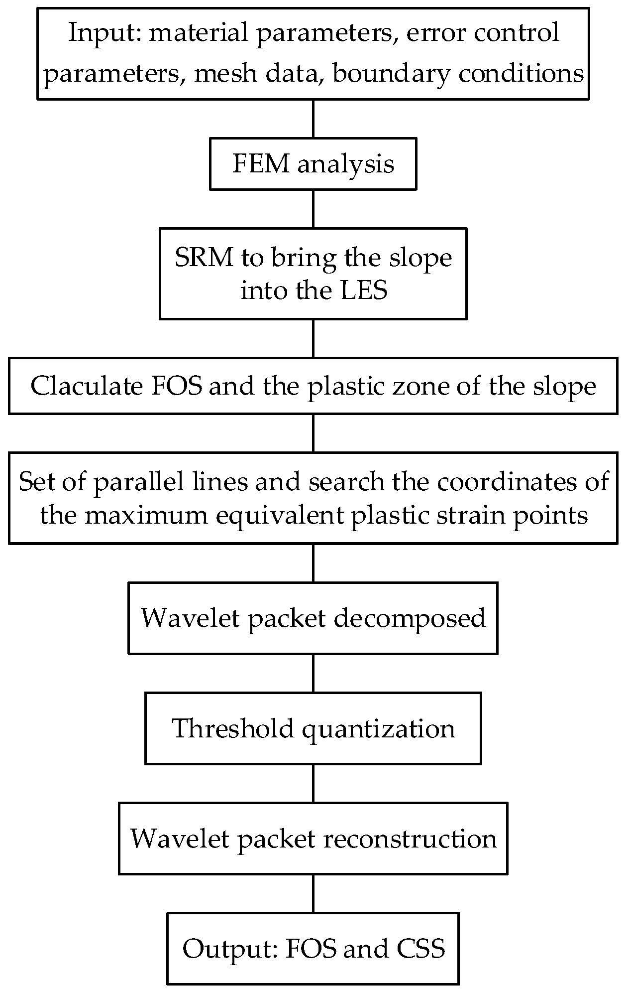
The implementation of the proposed method is summarized in the flow chart as in Figure 2.
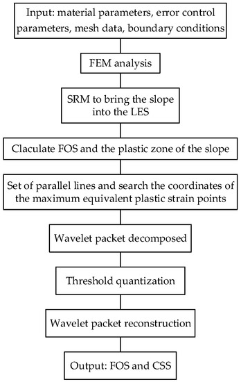
Figure 2.
Flow diagram for the proposed method.
5. Numerical Examples
Although more complicated constitutive models can be used in finite element analysis, the most commonly used model in engineering analysis is the elastic-perfectly plastic model based on Mohr–Coulomb’s yield criterion [41]. Therefore, in the following numerical example analysis, the Mohr–Coulomb’s yield surface and the associated flow rule were used in the material model. Pore pressure was not considered. Based on the plane strain assumption, the ANSYS software platform was used to simulate the slope with a four-node isoparametric element.
5.1. An Idealized Homogeneous Slope
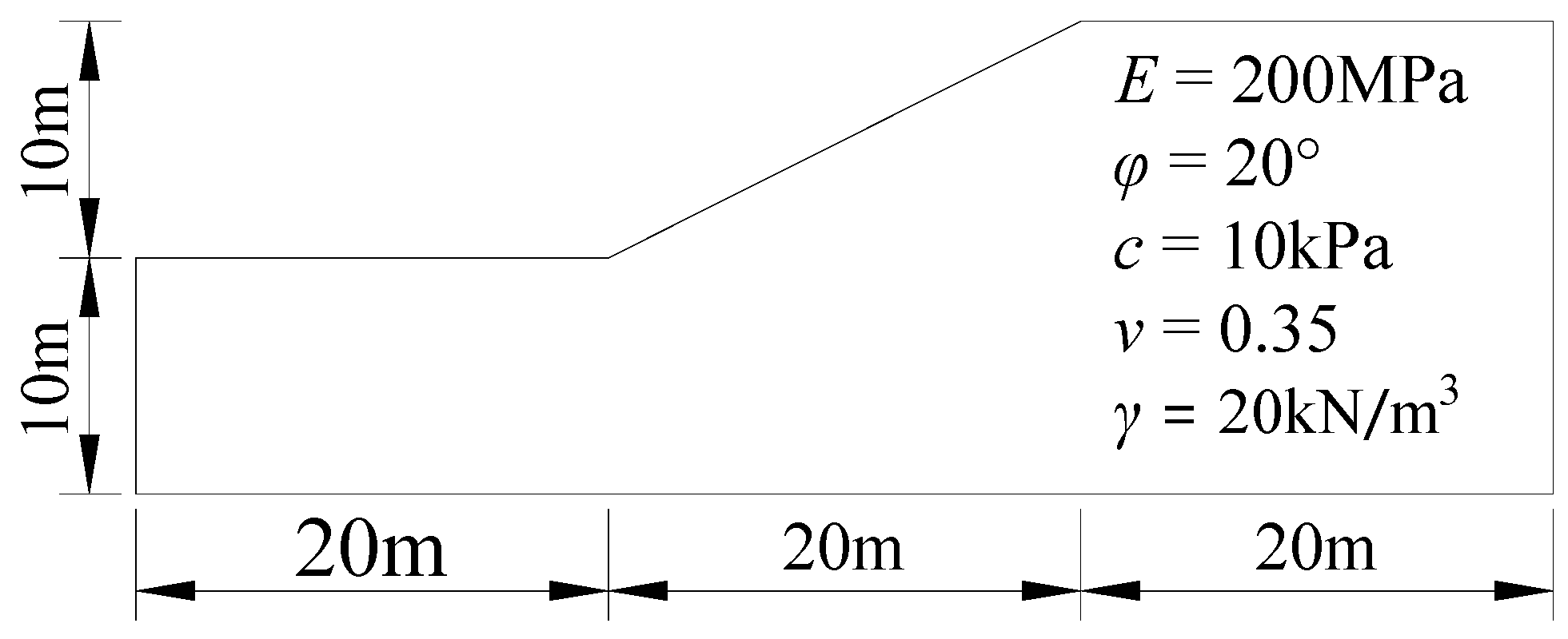
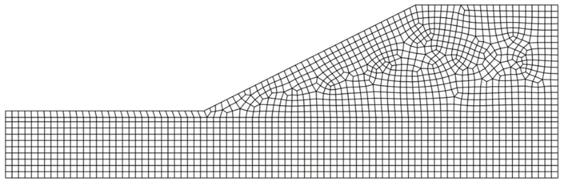
To verify the proposed method, a homogeneous slope studied in [58] was adopted, which was composed of homogeneous, isotropic soil. The dimensions and the material parameters of the slope are shown in Figure 3. Four discrete models were used to analyze the convergence of the proposed method, as shown in Figure 4, in which the boundary conditions of the computational models were as follows: the left and right boundaries were fixed in the horizontal direction, and the bottom boundary was fixed in the horizontal and vertical direction.
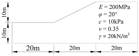
Figure 3.
Dimension of the model in Example 1.
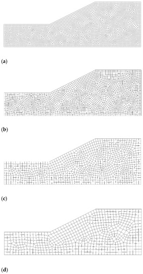
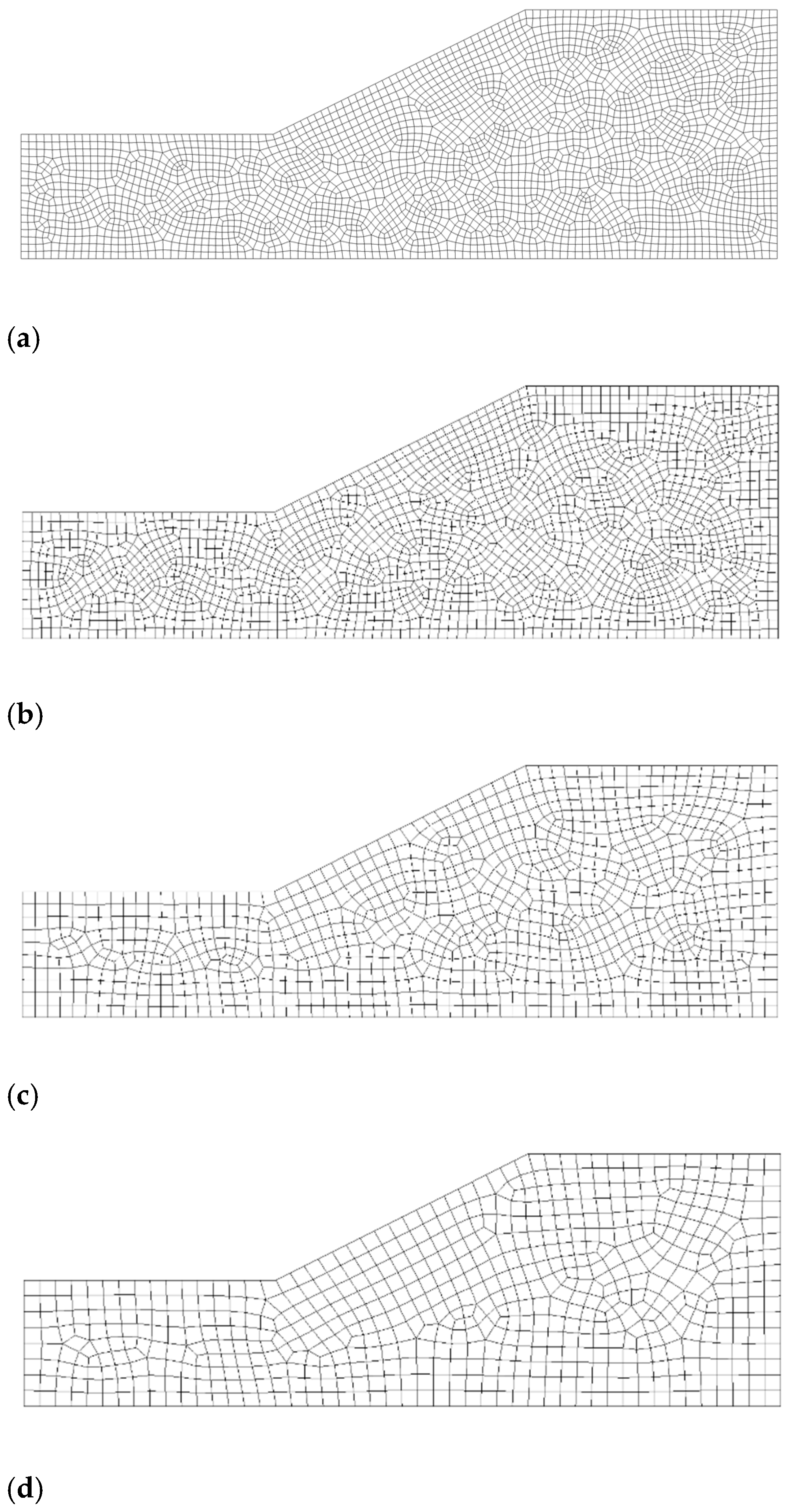
Figure 4.
Four discrete models for the homogeneous slope. (a) Model A (2955 elements); (b) Model B (1977 elements); (c) Model C (1065 elements); (d) Model D (640 elements).
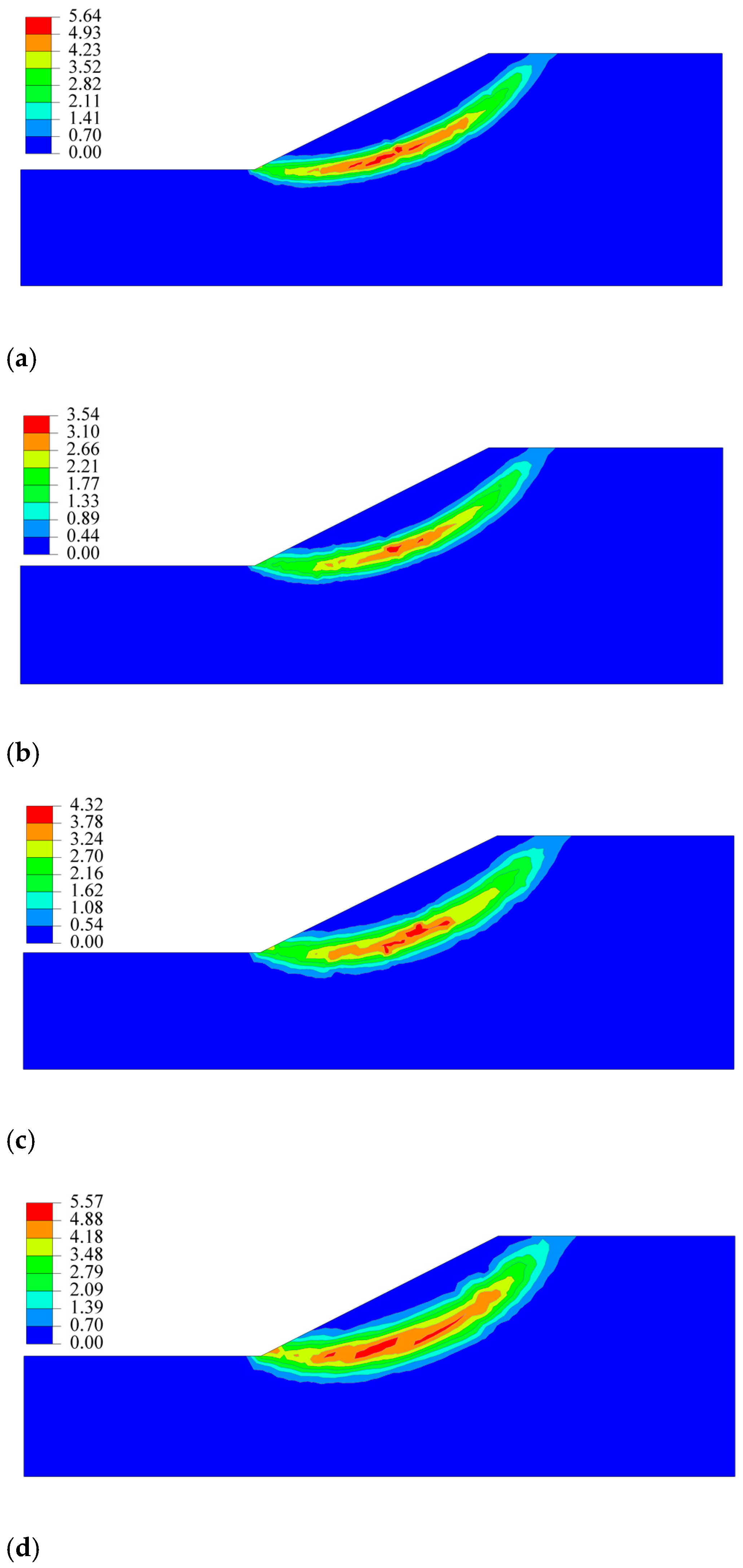
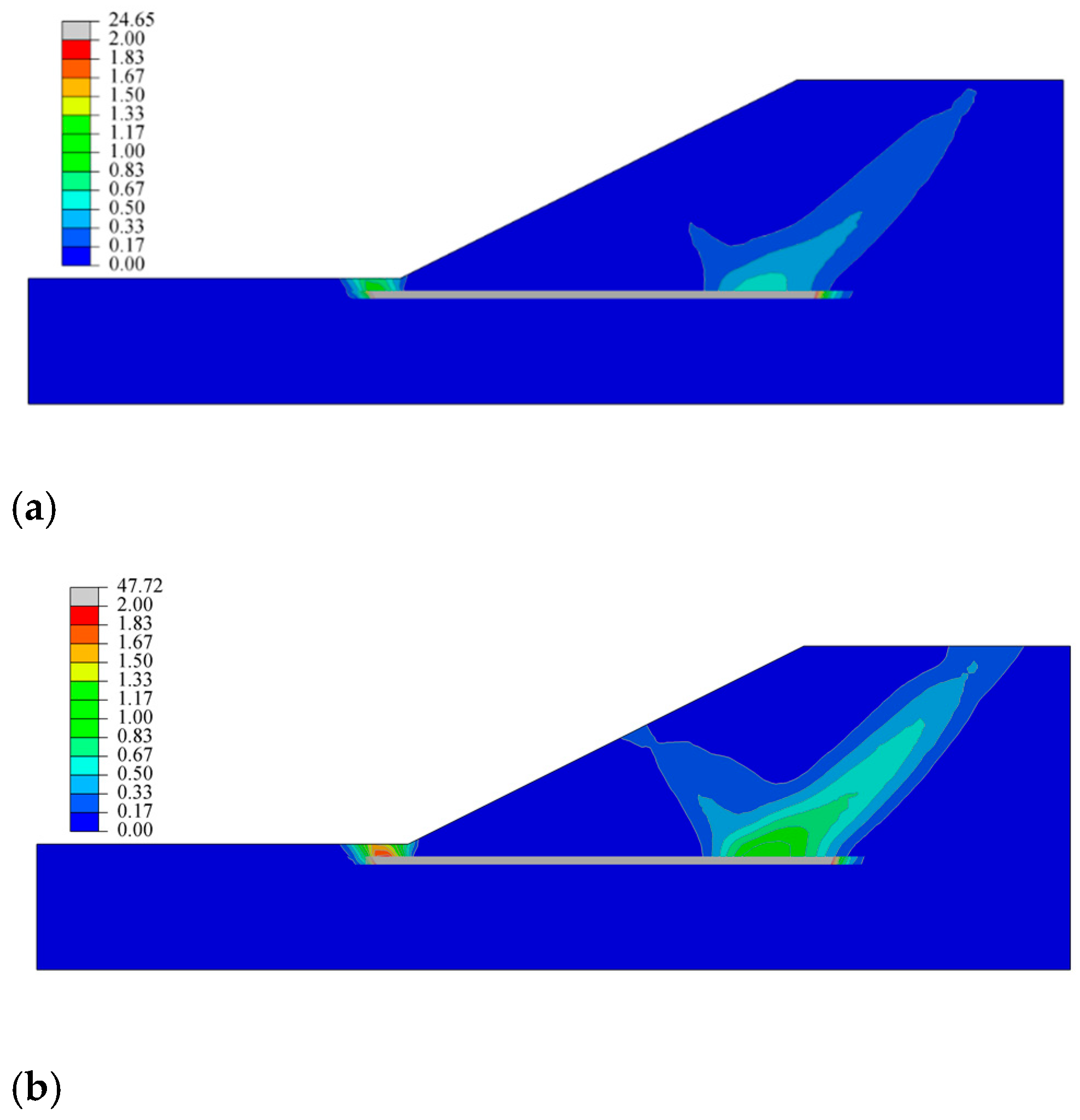
The EPS contours by the SRM using different models are plotted in Figure 5. The results indicate that the denser the mesh, the smaller the areas of the plastic zone. This is because of the mesh dependence of the FEM, which can be further proved by the distribution of maximum equivalent plastic strain, that is, the calculation model with denser mesh has lower data fluctuation. The traditional SRM can only give the contours of equivalent plastic strain as shown in Figure 5, and the specific position of the CSS cannot be given.

Figure 5.
The contours of equivalent plastic strain by the SRM. (a) Model A; (b) Model B; (c) Model C; (d) Model D.
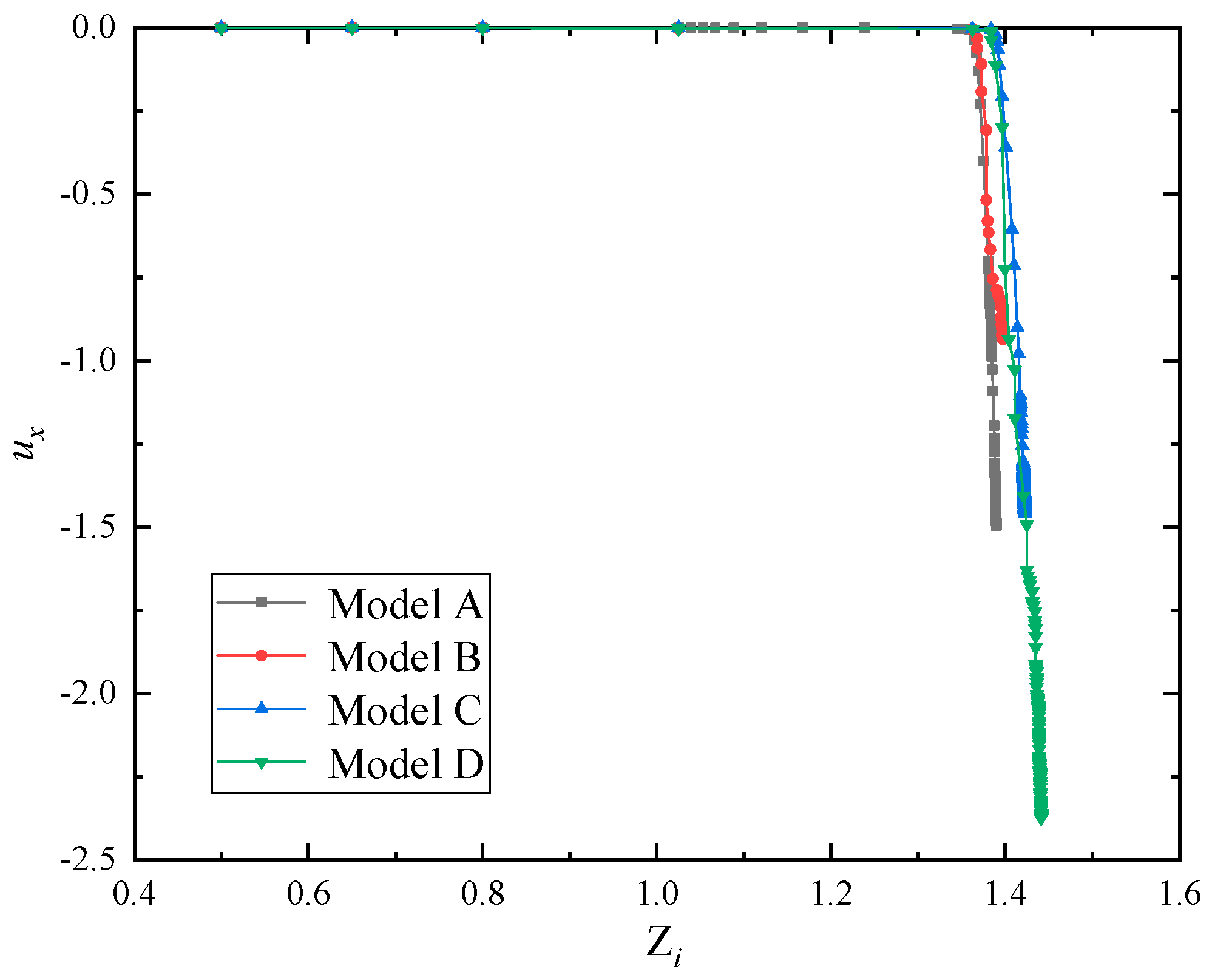
Taking the slope vertex node as a characteristic point, the reduction factor Zi versus horizontal displacement ux curve is drawn as shown in Figure 6. As can be seen from the figure, the horizontal displacement of the slope vertex node has an obvious inflection point.

Figure 6.
Reduction factor Zi versus the horizontal displacement ux curves.
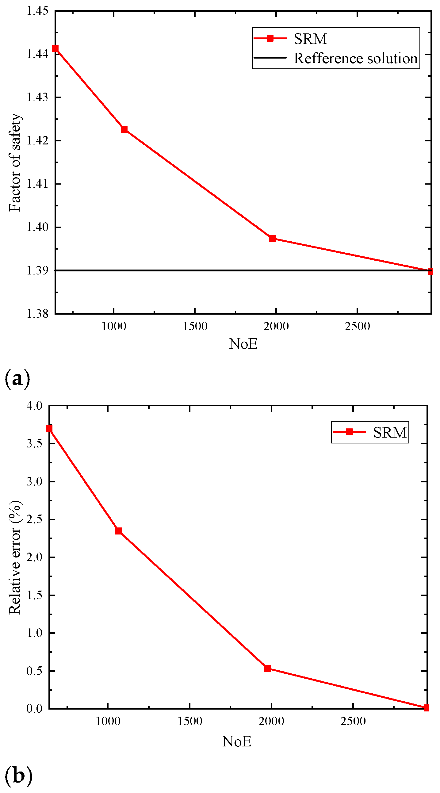
With the discretization of element length approximate to 0.6 m (Mesh A), 0.75 m (Mesh B), 1 m (Mesh C), and 1.25 m (Mesh D), the proposed procedure was given an FOS of 1.39, 1.40, 1.42, 1.44, respectively. The convergence curves of the numerical solution by the proposed method are plotted in Figure 7. Using an optimization process for the Spencer method in STAB, a software developed by Chen [58], the reference solution presented in Figure 7 is 1.39. As shown in Figure 7a, the model’s numerical solution gradually approached the reference solution as the number of elements (NoE) increases. In other words, the relative errors (Figure 7b) of FOS by the proposed method gradually decrease as the NoE increases.
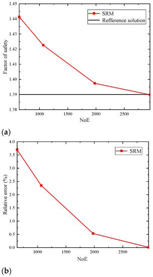
Figure 7.
The convergence of the numerical solution. (a) Convergence for the factor of safety. (b) Convergence of relative errors for the factor of safety.
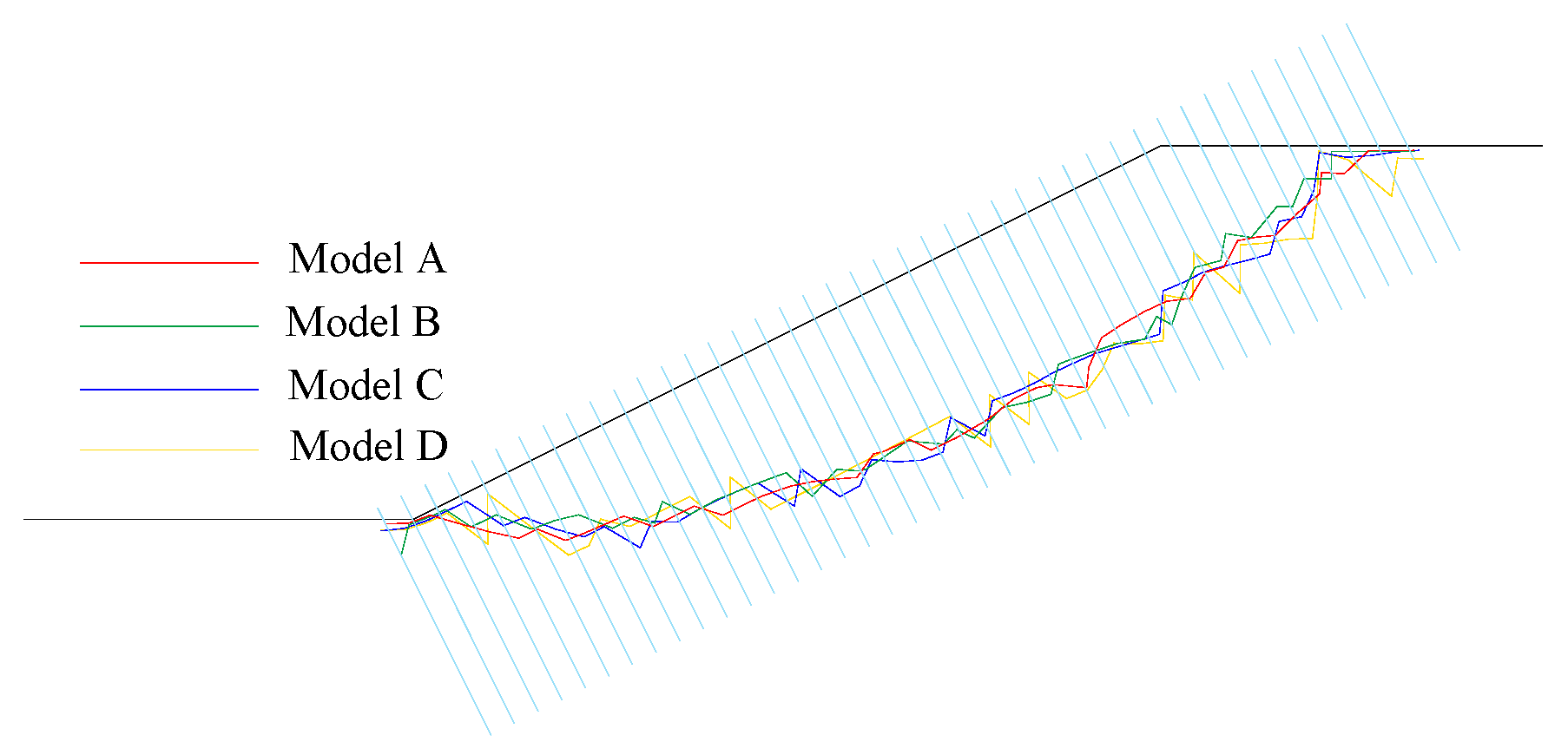
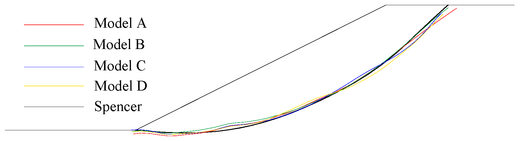
The slope toe was defined as the coordinate origin, X-axis along the slope surface, and Y-axis perpendicular to the slope surface. The distribution of the maximum equivalent plastic strains at the LES is illustrated in Figure 8, along with a direction perpendicular to the slope surface with an interval of 0.5 m. After the wavelet packet decomposition of the signal function, it could be observed that the high-frequency part of the signal was mainly concentrated in the first three orders. The CSS is obtained through a wavelet packet filter with db6 at the third scale level and the CSS in the LES are given in Figure 9. As shown in Figure 9, using different mesh density calculation models, the CSSs obtained by the proposed method are in good agreement with the Spencer method. The results show that the proposed method can overcome the mesh dependence of FEM, and it is reasonable to take the point with the maximum equivalent plastic strain point as the location of the CSS.
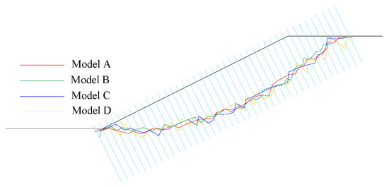
Figure 8.
The distribution of maximum equivalent plastic strain for Example 1.
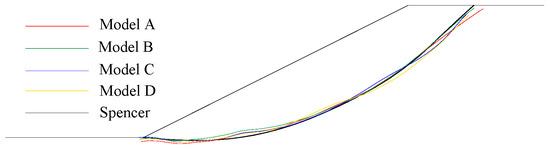
Figure 9.
Critical slip surfaces based on wavelet packet and Spencer for Example 1.
5.2. Slope Containing Weak Intercalated Layer
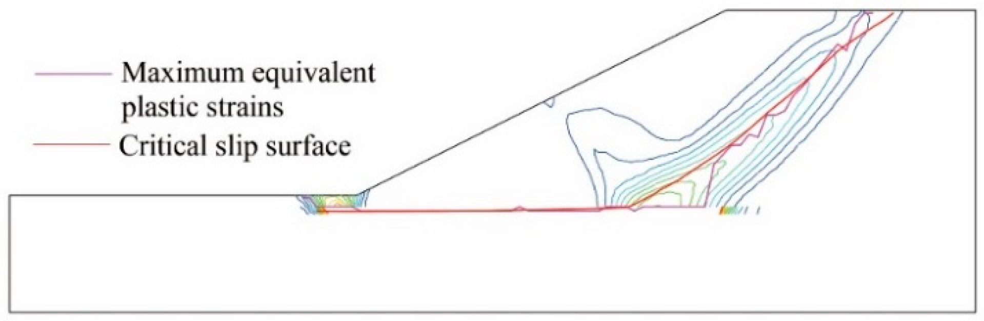
This example is Problem 3a issued by Australia Computer Association and Design Society (ACADS) [58,59,60,61] and is selected to verify that the proposed method can also accommodate inhomogeneous slopes. The slope geometry and the soil properties are illustrated in Figure 10. The mesh generation of the slope model is shown in Figure 11, and its boundary displacement constraints are the same as in Example 1. The contours of EPS by the SRM are plotted in Figure 12. As shown in Figure 12, the plastic zone first appeared in the weak interlayer, and the areas of the plastic zone increased as the reduction factor Fi increased. As Figure 13 shows, if a group of parallel lines are arranged with an interval of 0.6 m, the distribution of the maximum equivalent plastic strains is irregular. The analysis results are shown in Figure 13 and Figure 14 with db6 at the third scale level and are consistent with the Spencer method. According to the proposed method, the FOS is 1.31, which is close to the reference results of 1.24–1.27 given by ACADS [58].
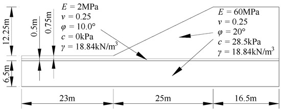
Figure 10.
Dimension of the model in Example 2.
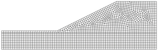
Figure 11.
Mesh for Example 2.

Figure 12.
The contours of equivalent plastic strain by the SRM for Example 2. (a) Fi = 1.15; (b) Fi = 1.31.

Figure 13.
The contour of equivalent plastic strain, distribution of the maximum equivalent plastic strains, and the CSS for Example 2.
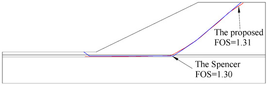
Figure 14.
Critical slip surfaces based on wavelet packet and Spencer for Example 2.
5.3. An Example of Soil-Rock Mixture Slope
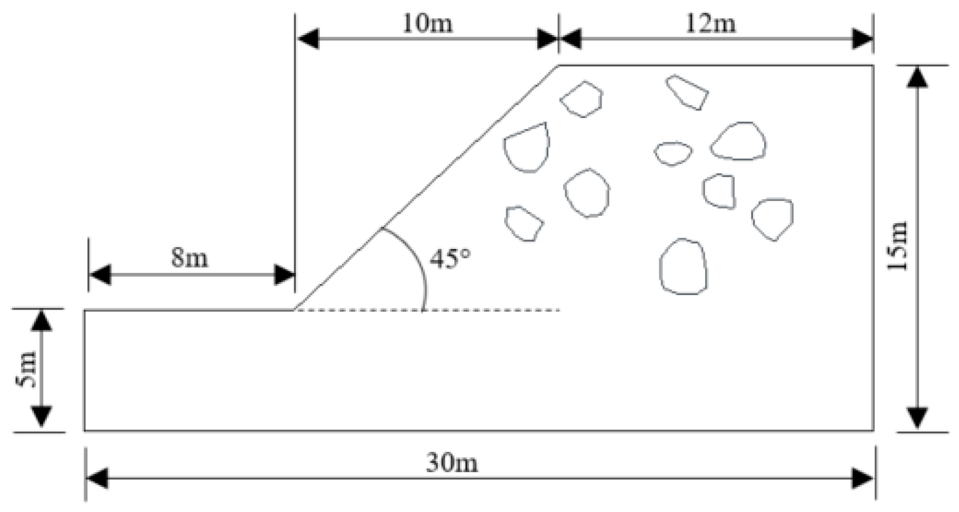
Figure 15 illustrates the geometric model size of the soil–rock mixture slope [12] and the material parameters are given in Table 1. The rock gradation of the soil–rock mixture slope is shown in Table 2.
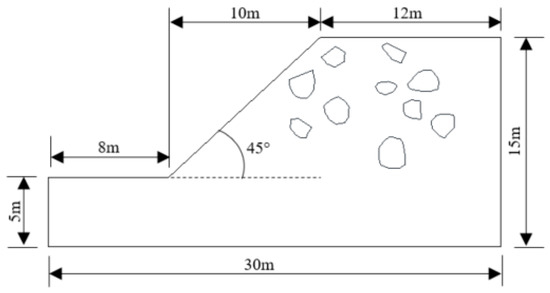
Figure 15.
Geometric parameters for Example 3: soil–rock mixture slope.

Table 1.
Material parameters.
Table 2.
Material parameters. Gradation of rock blocks for the soil–rock mixture slopes with different contents of rock blocks.
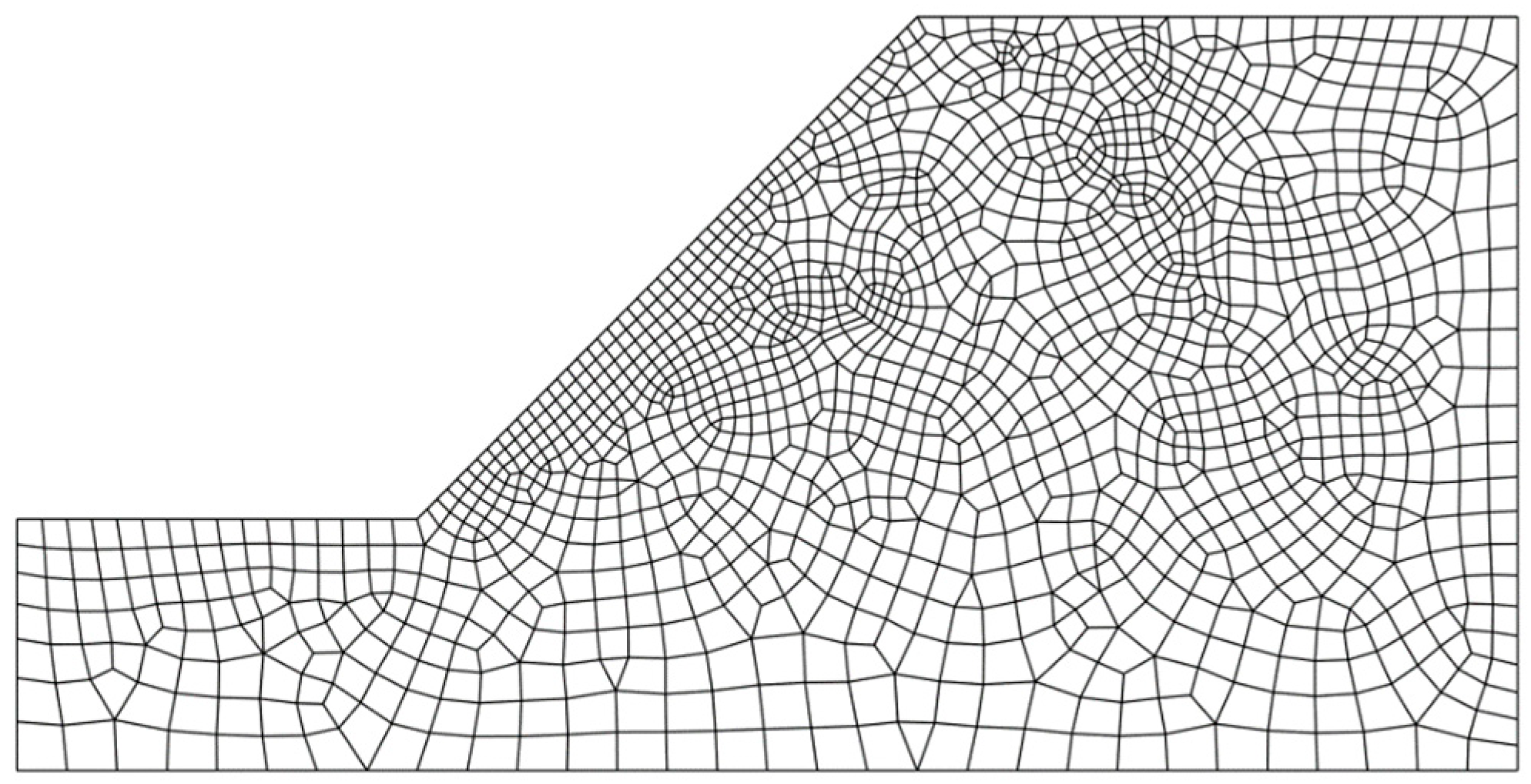
Figure 16 illustrates the mesh of the soil–rock mixture slope in ANSYS. By encrypting the mesh near the slope, more data points are available to be searched by the algorithm to improve the accuracy of the calculation and reduce the fluctuation of the equivalent plastic strain maximum distribution line, thus improving the smoothness of the slip surface by filtering with wavelets and reflecting more accurately the position of the CSS in the slope.

Figure 16.
The irregular mesh for the soil-rock mixture slope.
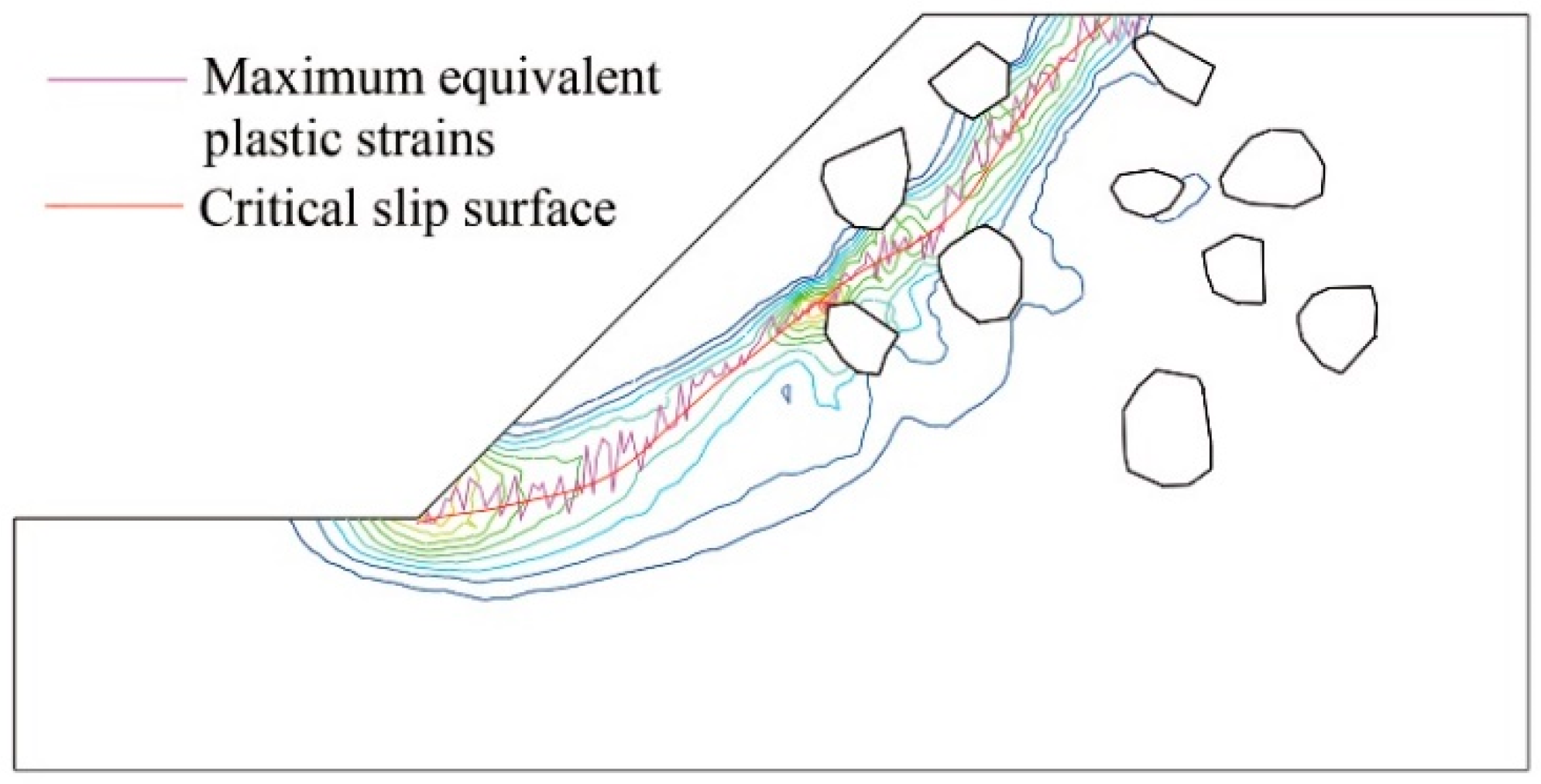
For this numerical example, the traditional LEM was no longer used. Therefore, the results of the proposed method were compared with the virtual element method [12]. The EPS contours by SRM are plotted in Figure 17. The plastic zone first appeared at the toe of the slop. With the increase in the reduction factor Fi, the stress concentration gradually appeared at the toe of the slope and around the stone, and finally, the plastic zone bypassed the stone. The failure mechanism was different from that of the soil slope. With an interval of 0.5 m, Figure 18 displays the distribution of the maximum equivalent plastic strains and CSS. Due to the traditional SRM, the specific location for CSS was also not given in [12]. A wavelet packet decomposition with a db4 scale of a fourth was performed on the data for this example to calculate the curve of the CSS. An FOS of 1.09 was generated, which is close to the 1.07 evaluated by Sun et al. [12]. The filtered fitted curve reflects the influence of the stones on the position of the CSS in stony soil slopes.
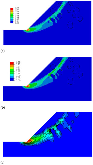
Figure 17.
The contours of equivalent plastic strain by the SRM for Example 3. (a) Fi = 0.95. (b) Fi = 1.09. (c) Fi = 1.07 [12].
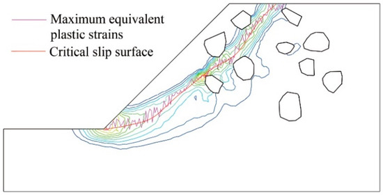
Figure 18.
The contour of equivalent plastic strain, distribution of the maximum equivalent plastic strains, and the CSS for Example 3.
6. Conclusions
To accurately locate the position of the CSS of a complicated slope in LES, a new method is proposed by combining the WPA and the SRM. The algorithm proposed in this paper includes two approaches. The first approach is an algorithm to bring the slope into the LES. Based on the SRM, the strain field of LES and FOS can be found. The second approach is the wavelet packet filter algorithm for smoothing the CSS. This algorithm applies wavelet packets to SSA. Through the analysis of three different examples and comparison with Spencer’s method, the results show that: (1) the proposed method is reasonable and efficient and can be used to locate the CSS; (2) it is reasonable to take the maximum equivalent plastic strain point as the position of CSS. It should be pointed out that this study is limited to two-dimensional SSA with elastic-perfectly plastic material. The validation of the proposed method for the three-dimensional problems and the non-elastic-perfectly plastic material needs further study.
Author Contributions
Conceptualization, Y.C.; Data curation, Z.N.; Formal analysis, C.H. and S.D.; Funding acquisition, Y.C.; Investigation, K.L.; Methodology, Z.N.; Project administration, Z.N.; Supervision, Y.C. All authors have read and agreed to the published version of the manuscript.
Funding
This study is supported by the National Key Research and Development Program of China, under the Grant Nos. 2018YFC0809400.
Institutional Review Board Statement
Not applicable.
Informed Consent Statement
Not applicable.
Data Availability Statement
All data included in this study are available upon request by contact with the corresponding author.
Conflicts of Interest
The authors declare no conflict of interest.
References
- Clough, R.W.; Woodward, R.J. Analysis of embankment stresses and deformations. J. Soil Mech. Found. Div. 1967, 93, 529–549. [Google Scholar] [CrossRef]
- Bishop, A.W. The Use of Pore-Pressure Coefficients in Practice. Géotechnique 1954, 4, 148–152. [Google Scholar] [CrossRef]
- Duncan, J.M. State of the art: Limit equilibrium and finite-element analysis of slopes. J. Geotech. Eng. 1996, 122, 577–596. [Google Scholar] [CrossRef]
- Zienkiewicz, O.C.; Humpheson, C.; Lewis, R.W. Associated and non-associated visco-plasticity and plasticity in soil mechanics. Geotechnique 1975, 25, 671–689. [Google Scholar] [CrossRef]
- Naylor, D.J. Finite Elements and Slope Stability. In Numerical Methods in Geomechanics; Springer: Dordrecht, The Netherlands, 1982. [Google Scholar]
- Wong, F.S. Uncertainties in FE modeling of slope stability. Comput. Struct. 1984, 19, 777–791. [Google Scholar] [CrossRef]
- Donald, I.B.; Giam, S.K. Application of the nodal displacement method to slope stability analysis. In Proceedings of the Australia-New Zealand Conference on Geomechanics, Sydeny, Australia, 22–26 August 1988; pp. 456–460. [Google Scholar]
- Matsui, T.; San, K.C. Finite element slope stability analysis by shear strength reduction technique. Soils Found. 1992, 32, 59–70. [Google Scholar] [CrossRef] [Green Version]
- Sun, G.H.; Cheng, S.G.; Jiang, W.; Zheng, H. A global procedure for stability analysis of slopes based on the Morgenstern-Price assumption and its applications. Comput. Geotech. 2016, 80, 97–106. [Google Scholar] [CrossRef]
- Griffiths, D.V.; Lane, P.A. Slope stability analysis by finite elements. Géotechnique 1999, 49, 387–403. [Google Scholar] [CrossRef]
- Baghini, E.G.; Toufigh, M.M.; Toufigh, V. Mesh-free analysis applied in reinforced soil slopes. Comput. Geotech. 2016, 80, 322–332. [Google Scholar] [CrossRef]
- Sun, G.H.; Lin, S.; Zheng, H.; Tan, Y.Z.; Sui, T. The virtual element method strength reduction technique for the stability analysis of stony soil slopes. Comput. Geotech. 2020, 119, 103349. [Google Scholar] [CrossRef]
- Nie, Z.B.; Zhang, Z.H.; Zheng, H. Slope stability analysis using convergent strength reduction method. Eng. Anal. Bound. Elem. 2019, 108, 402–410. [Google Scholar] [CrossRef]
- Nie, Z.B.; Zhang, Z.H.; Zheng, H.; Lin, S. Stability analysis of landslides using BEM and variational inequality based contact model. Comput. Geotech. 2020, 123, 103575. [Google Scholar] [CrossRef]
- Choi, S.K.; Park, J.Y.; Lee, D.H.; Lee, S.R.; Kim, Y.T.; Kwon, T.H. Assessment of barrier location effect on debris flow based on smoothed particle hydrodynamics (SPH) simulation on 3D terrains. Landslides 2021, 18, 217–234. [Google Scholar] [CrossRef]
- Conte, E.; Pugliese, L.; Troncone, A. Post-failure analysis of the Maierato landslide using the material point method. Eng. Geol. 2020, 277, 105788. [Google Scholar] [CrossRef]
- Troncone, A.; Pugliese, L.; Conte, E. Run-Out Simulation of a Landslide Triggered by an Increase in the Groundwater Level Using the Material Point Method. Water 2020, 12, 2817. [Google Scholar] [CrossRef]
- Xu, W.J.; Xu, Q.; Liu, G.Y.; Xu, H.Y. A novel parameter inversion method for an improved DEM simulation of a river damming process by a large-scale landslide. Eng. Geol. 2021, 293, 106282. [Google Scholar] [CrossRef]
- Yang, Y.T.; Sun, G.H.; Zheng, H. Investigation of the sequential excavation of a soil-rock-mixture slope using the numerical manifold method. Eng. Geol. 2019, 256, 93–109. [Google Scholar] [CrossRef]
- Li, Y.; Qian, C.; Fu, Z.; Li, Z. On Two Approaches to Slope Stability Reliability Assessments Using the Random Finite Element Method. Appl. Sci. 2019, 9, 4421. [Google Scholar] [CrossRef] [Green Version]
- Volpe, E.; Ciabatta, L.; Salciarini, D.; Camici, S.; Cattoni, E.; Brocca, L. The Impact of Probability Density Functions Assessment on Model Performance for Slope Stability Analysis. Geosciences 2021, 11, 322. [Google Scholar] [CrossRef]
- Cai, F.; Nakamura, A.; Ugai, K. Revisiting the three-dimensional slope stability problem in clay. Cancer Geotech. J. 2012, 49, 494–498. [Google Scholar] [CrossRef]
- Gao, Y.; Yang, S.; Zhang, F.; Leshchinsky, B. Three-dimensional reinforced slopes: Evaluation of required reinforcement strength and embedment length using limit analysis. Geotext. Geomembr. 2016, 44, 133–142. [Google Scholar] [CrossRef]
- Liu, H. The Influence of Initial Normal Stress Assumption of Slip Surface on Safety Factor of Symmetrical Three-Dimensional Slopes. Adv. Mater. Sci. Eng. 2019, 5, 1–8. [Google Scholar] [CrossRef] [Green Version]
- He, Y.; Liu, Y.; Zhang, Y.; Yuan, R. Stability assessment of three-dimensional slopes with cracks. Eng. Geol. 2019, 252, 136–144. [Google Scholar] [CrossRef]
- Lin, H.D.; Wang, W.C.; Li, A.J. Investigation of dilatancy angle effects on slope stability using the 3D finite element method strength reduction technique. Comput. Geotech. 2020, 118, 103295. [Google Scholar] [CrossRef]
- Palazzolo, N.; Peres, D.; Bordoni, M.; Meisina, C.; Creaco, E.; Cancelliere, A. Improving Spatial Landslide Prediction with 3D Slope Stability Analysis and Genetic Algorithm Optimization: Application to the Oltrepò Pavese. Water 2021, 13, 801. [Google Scholar] [CrossRef]
- Meng, J.; Mattsson, H.; Laue, J. Three-dimensional slope stability predictions using artificial neural networks. Int. J. Numer. Anal. Met. 2021, 45, 1988–2000. [Google Scholar] [CrossRef]
- Sun, G.H.; Yang, Y.T.; Cheng, S.G.; Zheng, H. Phreatic Line Calculation and Stability Analysis of Slopes under the Combined Effect of Reservoir Water Level Fluctuations and Rainfall. Cancer Geotech. J. 2017, 54, 631–645. [Google Scholar] [CrossRef] [Green Version]
- Sun, G.H.; Wang, W.; Shi, L. Steady seepage analysis in soil-rock-mixture slope using the numerical manifold method. Eng. Anal. Bound. Elem. 2021, 131, 27–40. [Google Scholar] [CrossRef]
- Ma, Z.; Liao, H.; Dang, F.; Cheng, Y. Seismic slope stability and failure process analysis using explicit finite element method. Bull. Eng. Geol. Environ. 2020, 80, 1–15. [Google Scholar] [CrossRef]
- Metya, S.; Bhattacharya, G. Accounting for 2D Spatial Variation in Slope Reliability Analysis. Int. J. Geomech. 2020, 20, 04019190.1–04019190.16. [Google Scholar] [CrossRef]
- Kang, S.; Lee, S.; Cho, S. Slope Stability Analysis of Unsaturated Soil Slopes Based on the Site-Specific Characteristics: A Case Study of Hwangryeong Mountain, Busan, Korea. Sustainability 2020, 12, 2839. [Google Scholar] [CrossRef] [Green Version]
- Wang, S.; Zhao, M.; Meng, X.; Chen, G.; Zeng, R.; Yang, Q.; Liu, Y.; Wang, B. Evaluation of the Effects of Forest on Slope Stability and Its Implications for Forest Management: A Case Study of Bailong River Basin, China. Sustainability 2020, 12, 6655. [Google Scholar] [CrossRef]
- Huang, G.; Zheng, M.; Peng, J. Effect of Vegetation Roots on the Threshold of Slope Instability Induced by Rainfall and Runoff. Geofluids 2021, 1, 1–19. [Google Scholar]
- Khan, M.; Wang, S. Slope Stability Analysis to Correlate Shear Strength with Slope Angle and Shear Stress by Considering Saturated and Unsaturated Seismic Conditions. Appl. Sci. 2021, 11, 4568. [Google Scholar] [CrossRef]
- Azmoon, B.; Biniyaz, A.; Liu, Z. Evaluation of Deep Learning against Conventional Limit Equilibrium Methods for Slope Stability Analysis. Appl. Sci. 2021, 11, 6060. [Google Scholar] [CrossRef]
- Lechman, J.B.; Griffiths, D.V. Analysis of the Progression of Failure of Earth Slopes by Finite Elements. In Proceedings of the Geo-Denver 2000, Denver, CO, USA, 5–8 August 2000; pp. 250–265. [Google Scholar]
- Dawson, E.; Motamed, F.; Nesarajah, S.; Roth, W. Geotechnical Stability Analysis by Strength Reduction. In Proceedings of the Geo-Denver 2000, Denver, CO, USA, 5–8 August 2000; pp. 99–113. [Google Scholar]
- Zheng, H.; Sun, G.H.; Liu, D.F. A practical procedure for searching critical slip surfaces of slopes based on the strength reduction technique. Comput. Geotech. 2009, 36, 1–5. [Google Scholar] [CrossRef]
- Zheng, H.; Liu, D.F.; Li, C.G. Slope stability analysis based on elasto-plastic finite element method. Int. J. Numer. Meth. Eng. 2005, 64, 1871–1888. [Google Scholar] [CrossRef]
- Nie, Z.B.; Zheng, H.; Zhang, T. Determination of slope critical slip surfaces using strength reduction method and wavelet transform. Rock Soil Mech. 2017, 38, 1827–1831. (In Chinese) [Google Scholar]
- Yong, R. An Introduction to Nonlinear Fourier Series; Academic: New York, NY, USA, 1980. [Google Scholar]
- Kim, H.S.; Melhem, H. Damage detection of structures by wavelet analysis. Eng. Struct. 2004, 26, 347–362. [Google Scholar] [CrossRef]
- Daubechies, I. The wavelet transform, time-frequency localization and signal analysis. IEEE Trans. Inf. Theory 1990, 36, 961–1005. [Google Scholar] [CrossRef] [Green Version]
- Coifman, R.R.; Donoho, D.L. Translation-Invariant De-Noising. Wavelets Stat. 1995, 103, 125–150. [Google Scholar]
- Guo, F.; Yang, Y.; Chen, B.; Guo, L. A novel multi-scale edge detection technique based on wavelet analysis with application in multiphase flows. Powder Technol. 2010, 202, 171–177. [Google Scholar] [CrossRef]
- Cohen, A. Numerical Analysis of Wavelet Methods. In Studies in Mathematics and Its Applications; North-Holland Publishing Co.: Amsterdam, The Netherlands, 2003; Volume 32. [Google Scholar]
- Abramson, L.W.; Lee, T.S.; Sharma, S.; Boyce, G.M. Slope Stability and Stabilization Methods; John Wiley: New York, NY, USA, 1996. [Google Scholar]
- Dawson, E.M.; Roth, W.H.; Drescher, A. Slope stability analysis by strength reduction. Geotechnique 1999, 49, 835–840. [Google Scholar] [CrossRef]
- Snitbhan, N.; Chen, W.F. Elastic-plastic large deformation analysis of soil slope. Comput. Struct. 1978, 9, 567–577. [Google Scholar] [CrossRef]
- Zheng, H.; Liu, D.F.; Li, C.G. On the Assessment of Failure in Slope Stability Analysis by the Finite Element Method. Rock Mech. Rock Eng. 2008, 41, 629. [Google Scholar] [CrossRef]
- Sun, Y.K. Wavelet Analysis and Its Application; China Machine Press: Beijing, China, 2005. (In Chinese) [Google Scholar]
- Yuan, T.T.; Liu, Q.; Ai, Q.S. Study on best wavelet packet based on independent threshold denoising for MUAP. In Proceedings of the 2010 Second World Congress on Software Engineering (WCSE), Wuhan, China, 19–20 December 2010; Volume 1, pp. 269–272. [Google Scholar]
- Walczak, B.; Massart, D.L. Noise Suppression and Signal Compression Using the Wavelet Packet Transform. Chemom. Intell. Lab. Syst. 1997, 36, 81–94. [Google Scholar] [CrossRef]
- Coifman, R.R.; Wickerhauser, M.V. Entropy-based algorithms for best basis selection. IEEE Trans. Inf. Theory 1992, 38, 713–718. [Google Scholar] [CrossRef] [Green Version]
- Gencay, R.; Selcuk, F.; Whitcher, B. An Introduction to Wavelets and Other Filtering Methods in Finance and Economics; Elsevier: Amsterdam, The Netherlands, 2001; Volume 12, pp. 202–234. [Google Scholar]
- Chen, Z.Y. Soil Slope Stability Analysis—Theory, Methods and Programs; China Water Power Press: Beijing, China, 2003. (In Chinses) [Google Scholar]
- Donald, I.B.; Giam, P.S.K. The ACADS slope stability programs review. In Proceedings of the 6th International Symposium on Landslides, Christchurch, New Zealand, 10–14 February 1992; Bell, D.H., Ed.; Elsevier: Amsterdam, The Netherlands, 1992; Volume 3, pp. 1665–1670. [Google Scholar]
- Guo, M.W.; Li, C.G.; Wang, S.L.; Yin, S.D.; Liu, S.J.; Ge, X.R. Vector-Sum Method for 2D Slope Stability Analysis Considering Vector Characteristics of Force. Int. J. Geomech. 2019, 19, 04019058. [Google Scholar] [CrossRef]
- Tang, H.M.; Liu, X.; Xiong, C.R.; Wang, Z.Y.; Eldin, M. Proof of Nondeterministic Polynomial-Time Complete Problem for Soil Slope-Stability Evaluation. Int. J. Geomech. 2016, 16, 12. [Google Scholar] [CrossRef]


Publisher’s Note: MDPI stays neutral with regard to jurisdictional claims in published maps and institutional affiliations. |
© 2021 by the authors. Licensee MDPI, Basel, Switzerland. This article is an open access article distributed under the terms and conditions of the Creative Commons Attribution (CC BY) license (https://creativecommons.org/licenses/by/4.0/).