Estimating the Epicenter of an Impending Strong Earthquake by Combining the Seismicity Order Parameter Variability Analysis with Earthquake Networks and Nowcasting: Application in the Eastern Mediterranean

Abstract

The variance ${\kappa }_1$ of the natural time analysis of earthquake catalogs was proposed in 2005 as an order parameter for seismicity, whose fluctuations proved, in 2011, to be minimized a few months before the strongest mainshock when studying the earthquakes in a given area. After the introduction of earthquake networks based on similar activity patterns, in 2012, the study of their higher order cores revealed, in 2019, the selection of appropriate areas in which the precursory minima ${\beta }_{min}$ of the fluctuations $\beta$ of the seismicity order parameter ${\kappa }_1$ could be observed up to six months before all strong earthquakes above a certain threshold. The eastern Mediterranean region was studied in 2019, where all earthquakes of magnitude $M\ge 7.1$ were found to be preceded by ${\beta }_{min}$ without any false alarm. Combining these results with the method of nowcasting earthquakes, introduced in 2016, for seismic risk estimation, here, we show that the epicenter of an impending strong earthquake can be estimated. This is achieved by employing—at the time of observing the ${\beta }_{min}$—nowcasting earthquakes in a square lattice grid in the study area and by averaging, self-consistently, the results obtained for the earthquake potential score. This is understood in the following context: The minimum ${\beta }_{min}$ is ascertained to almost coincide with the onset of Seismic Electric Signals activity, which is accompanied by the development of long range correlations between earthquake magnitudes in the area that is a candidate for a mainshock.

1. Introduction

The natural time analysis (NTA) was introduced in the early 2000s [1,2,3], and revealed hidden properties in the time series of complex systems that cannot be observed in conventional time; for a review, see, e.g., [4]. It has found applications in various disciplines ranging from statistical physics [5,6,7,8], solid state physics [9] and, rock physics [10] to environmental physics [11,12,13], cardiology [14,15,16,17,18], and engineering [19,20,21]. The NTA has also found various applications in the context of seismology and physics of earthquakes (EQs); see, e.g., [3,22,23,24,25,26,27,28,29,30,31,32,33,34,35,36,37,38,39,40,41,42,43,44,45]. Such an application is presented in this paper.

The EQs exhibit power law correlations in time, space, and magnitude (M) [46,47,48,49,50,51,52,53,54,55,56,57,58,59,60,61,62,63,64,65,66,67,68,69] that have been suggested [70,71] to indicate the proximity to a critical point [72,73,74,75,76]. Several proposals suggest [73,74,77] that the EQ dynamics are associated with a second-order phase transition, or with a mean-field spinodal [76] that can be understood as a line of critical points. A first-order phase transition (see, e.g., [78] and references therein) has also been proposed as an alternative. In phase transitions, the new phase corresponds to the mainshock and a quantity-termed order parameter is required to correctly identify the new phase. Landau and Lifshitz [79] state: “To describe quantitatively the change in the structure of the body when it passes through the phase transition point, we can define a quantity $\eta$, called the order parameter, in such a way that it takes non-zero (positive or negative) values in the unsymmetrical phase and is zero in the symmetrical phase”.

Along these lines, Varotsos et al. [23] proposed the variance ${\kappa }_1$ of the NTA of EQ catalogs as an order parameter for seismicity. As such, it is non-zero before the mainshock, falling abruptly to zero upon its occurrence (see, e.g., the last points in Figure 6 by Márquez et al. [80]) and its scaled distribution exhibits a behavior similar to that of other equilibrium and non-equilibrium critical systems [7,21,23,28,81]. Later, it was shown that, when studying the EQs in a given area, the fluctuations $\beta$ of this order parameter were minimized a few months before the strongest mainshock [82], and the experimental results revealed that such minima occurred almost simultaneously with the observation of Seismic Electric Signals (SES) activities [83], which are series of low frequency ($f\le$1 Hz) electric signals that precede strong EQs [84,85,86,87,88,89,90]. Subsequent studies have shown that such minima are observed before strong EQs, both regionally [29] and globally [91]. These minima were found to be statistically significant precursors of EQs [92,93,94]. Furthermore, Varotsos et al. [95] showed that regional ${\beta }_{min}$ in Japan is observed when long-range correlations develop between EQ magnitudes, which has also been verified in two recent strong EQs in the Americas [40,96].

In recent decades, the theory of networks [97,98,99,100,101] has triggered many applications in seismicity (see, e.g., [47,60,102,103,104,105,106,107,108]), which showed that the EQ network properties may reveal a seismic hazard [109,110,111,112,113,114]. Tenenbaum et al. [60] introduced the EQ networks based on similar activity patterns (ENBOSAP) which are very useful for the NTA of seismicity [83]. Furthermore, the study of the higher order cores of these networks allowed the selection of appropriate areas in which the precursory minima ${\beta }_{min}$ of the fluctuations of the seismicity order parameter ${\kappa }_1$ can be observed up to six months before all strong mainshocks above a certain threshold [115]. In particular, the case studied in 2019 was the eastern Mediterranean region and resulted in five precursory ${\beta }_{min}$ before all EQs of magnitude $M\ge 7.1$ without false alarms.

It is the scope of the present paper to show that by combining the above two NTA results with the modern method of nowcasting EQs [33], an estimate of the epicenter of the impending EQ with $M\ge 7.1$ in the eastern Mediterranean region is achieved. EQ nowcasting employs natural time, which is unique in its characteristics [116], to estimate seismic risk by means of an EQ potential score (EPS) and found many useful applications, both regionally and globally [33,116,117,118,119,120,121,122,123,124,125,126]. EQ nowcasting [33] has, so far, focused on describing the current state of fault systems.

2. Materials and Methods

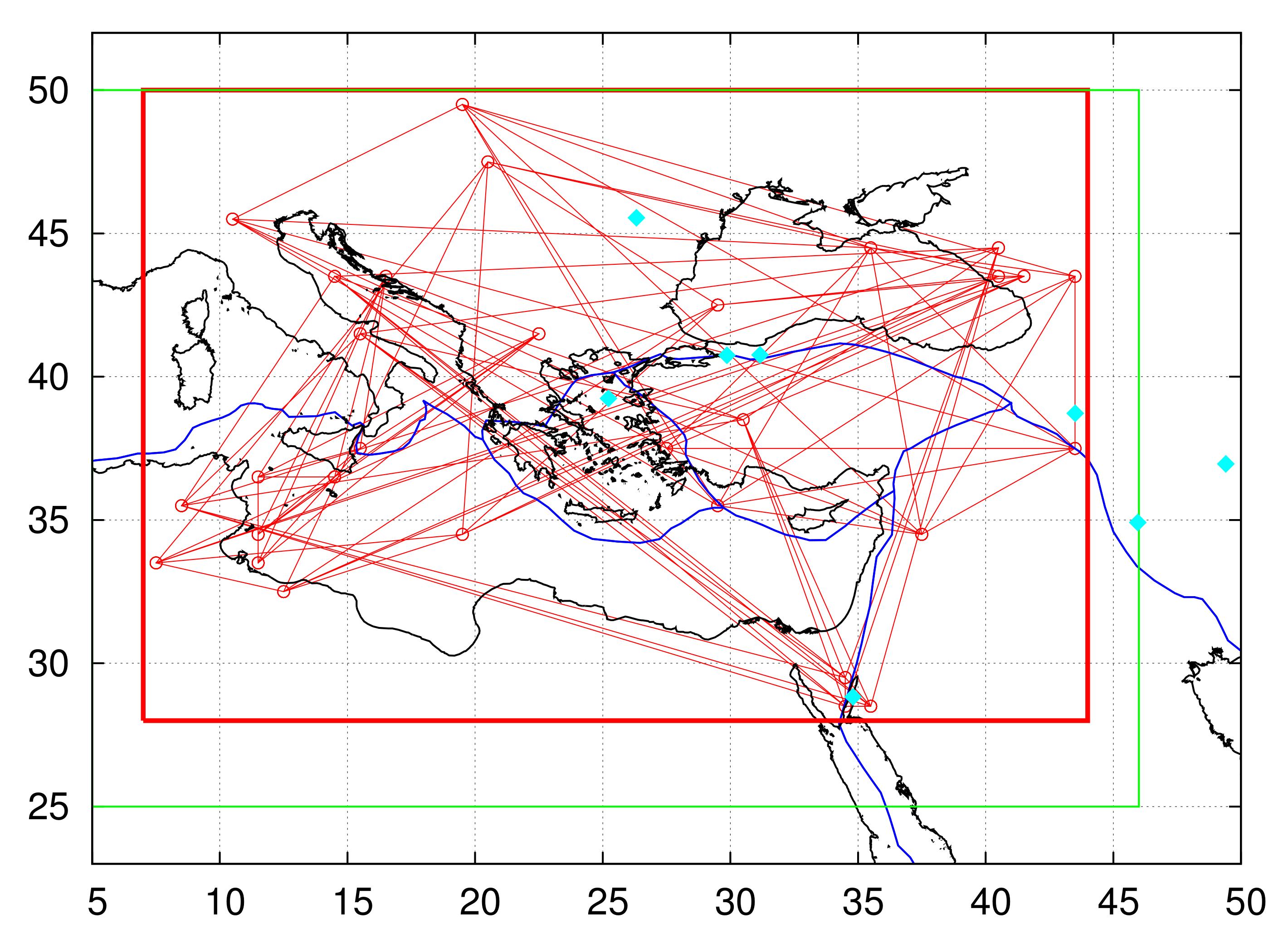
2.1. Study Area and EQ Data

Here, the area of interest was the eastern Mediterranean, see Figure 1. We used the United States National Earthquake Information Center (NEIC) PDE catalog—the data available from the United States Geological Survey (USGS), cf. [127]—in the region N${}_{23}^{52}$E${}_5^{50}$, and considered all EQs recorded during the period of almost 45 years from November 1976 to February 2021 with ${\mathrm{M}}_{thres}=3.8$. The eastern Mediterranean Sea and its surrounding coastal areas of Greece and western Turkey are one of the most seismically active and rapidly deformed regions on the continents [128]. This area is tectonically dominated by the relative plate motions between Eurasia and African lithosphere plates and their microplates. The African plate moves north to Eurasia from Gibraltar to the east. The plate boundary crosses North Africa and continues into southern Sicily, continuing around the Adriatic through Italy and eastern Balkans to Albania and northwestern Greece. There is a suggestion that the Adriatic is part of the African plate forming a small plate called Apulia [129]. The Apulia plate has a continental structure, e.g., it has a similar mean density to the density of the Eurasian plate, and their interaction leads to a continental collision. This microplate is suggested to rotate counter clockwise and its interaction with Eurasia is responsible for the shallow EQs in the region of Croatia, Albania and northwestern Greece. East of Apulia, the rapid movement of two small plates, the Aegean and the Turkish, takes up the relative movement between the Eurasia and African plates. The Aegean plate consists of the Aegean Sea, part of the Greek peninsula, Crete, and part of the western area of Asia Minor, while the Turkish part includes most of Asia Minor and Cyprus. The collision between Arabia and Eurasia in the Caucasus and eastern Turkey forces the Turkish plate to move westward in relation to Eurasia. Due to this movement, the strain accumulates along the North Anatolian transform fault (e.g., the opposite sides of this fault belong to different plates that move horizontally on top of each other) that accommodates large destructive EQs. The northern front of the African plate, south of the Adriatic Sea, forms the eastern Mediterranean oceanic lithosphere. As this oceanic lithosphere has a higher density than the continental lithosphere of the Aegean plate, it sinks below it, with an average angle of 38${}^{\circ }$, and forms the Hellenic Arc (SW of Cefallonia to S. Peloponnese, S. Crete up to S. Rhodes) and is associated with a sharp crustal shortening and an uplift rate of a few mm/yr along the Hellenic Arc due to the accretion of sediments of the African plate below the overriding Aegean plate [130]. Most of the subduction movement is accommodated along the Hellenic arc causing shallow depth EQs at its outer part. The seismically active regions of western Turkey, eastern and northern Greece, and the northern Aegean Sea are dominated by extension forces such as the southern Aegean Sea move in an almost southwesterly direction relative to Eurasia. This extension is thought to be driven principally by the “roll-back” of the subducting slab below the southern Aegean, as it sinks into the mantle [131]. The geophysical properties are different in the Aegean Sea from those in the outer part of the Hellenic arc. Another geotectonic feature causing destructive EQs is the significant right-lateral strike-slip movement along the North Aegean trough, and the Cephalonia–Lefkada transform zone, which is due to the offset between the oceanic–continental convergence to the west and the westward propagation of the Anatolian plate to the east. The combination of all the above factors leads to a significant left-lateral movement along the southeastern front of the Aegean–African interface [130].

2.2. Minima of the Variability of the Order Parameter of Seismicity

In a time series comprising N EQs, the natural time ${\chi }_k$ for the occurrence of the k-th EQ of energy $Q_k$ is defined as ${\chi }_k=k/N$. This means that the time intervals between consecutive events are ignored, but their order, as well as their energy, $Q_k$ are preserved. In NTA, the evolution of the pair $({\chi }_k,p_k)$ is studied, where:

$$p_k=\frac{Q_k}{{\sum }_{n=1}^N{Q}_n}$$

(1)

is the normalized energy and $Q_k$ is estimated by means of the relation [133] $Q_k\propto {10}^{1.5M_k}$, where $M_k$ stands for the EQ magnitude. It has been argued [23], as mentioned in the Introduction, that the variance ${\kappa }_1=\langle {\chi }^2\rangle -{\langle \chi \rangle }^2$ of natural time $\chi$ weighted for $p_k$, namely:

$${\kappa }_1=\sum _{k=1}^N{p}_k{\left({\chi }_k\right)}^2-{\left(\sum _{k=1}^N{p}_k{\chi }_k\right)}^2,$$

(2)

can be considered as an order parameter for seismicity. The study of the fluctuations of this order parameter of seismicity in an EQ catalog was conducted through a fixed-length sliding natural time window containing a number W of consecutive EQs that would occur on average within the crucial scale [82] of a few months, or so, which is the average lead time of SES activities. Following the procedure described by [29,95], we estimated ${\kappa }_1$ from the subexcerpts of consecutive 6 to W EQs within the window of W EQs and, then, calculated the average value ${\mu }_W\left({\kappa }_1\right)$ and the standard deviation ${\sigma }_W\left({\kappa }_1\right)$ of the obtained ${\kappa }_1$ values. The quantity:

$${\beta }_W\equiv \frac{\sigma {}_W\left({\kappa }_1\right)}{\mu {}_W\left({\kappa }_1\right)}$$

(3)

was termed [4,134] variability of ${\kappa }_1$. The temporal evolution of the ${\beta }_W$ value (Figure 2) could then be pursued by sliding the natural time window of W consecutive EQs, event by event, through the EQ catalog and assign to its value, the occurrence time of the EQ which follows the last EQ of the window in the EQ catalog. The corresponding minimum value was labeled ${\beta }_{W,min}$. The quantity ${\beta }_W$ of Equation (3) is reminiscent [115] of the square root of the Ginzburg criterion introduced in the context of the mean field theories of phase transitions of the Ginzburg–Landau type (see, e.g., p. 175 of Goldenfeld [135]). The latter criterion was also discussed by Holliday et al. [72].

To identify a precursory variability minimum [29,91,95], two window lengths, W and $W^{\prime }$ ($W^{\prime }>W$), corresponding to the number of EQs that occurred within a few months, were selected and ${\beta }_W$ and ${\beta }_{W^{\prime }}$ (sliding independently event by event) should have exhibited their local minima almost simultaneously. This meant that one required at least 90% of the EQs included in the calculation of the local ${\beta }_W$ minimum, and were also included in the calculation of the local ${\beta }_{W^{\prime }}$ minimum. Once this condition was valid, it was examined whether the ratio $r\equiv {\beta }_{W^{\prime },min}/{\beta }_{W,min}$ laid within the margins defined by the precursory to strong EQ variability minima; see, e.g., [29,91,95]. For example, for the area $A_6$ of Figure 1, the selection of $r\in (r_1=0.98,r_2=1.07)$ led to 7 variability minima (see Table 2 of [115]) when imposing a threshold ${\beta }_0=0.253$ below which the minima of ${\beta }_W$ for $W=80$ must be considered by the aforementioned procedure (cf. $W=80$ EQs corresponds to the number of EQs occurring on average in area $A_6$ of Figure 1 within two months).

2.3. Earthquake Networks Based on Similar Activity Patterns

Tenenbaum et al. [60] suggested the construction of the ENBOSAP as follows: The area under study was evenly spaced in geographical coordinates in “squares” of dimensions of about 100 km × 100 km, each marked by two integers $(i,j)$. The center of each “square” is a possible node of the network. The fact that EQs do not occur on a daily basis in every square makes it necessary to coarse-grain the seismic activity over a predefined time interval. There is a trade-off between precision and data richness leading [60] to an optimal coarseness in the 90-day time series. Thus, the seismic activity $s_t$ in each square covered 90 days and $s_{t+1}$ corresponded to the next 90 days of non-intersecting time periods, giving about 4 different values per year. The energy released in each 90-day period inside the “square” with indices $(i,j)$ was given by [60]:

$$s_t(i,j)\equiv \sum _{l=1}^{N_t(i,j)}{10}^{\frac{3}{2}{\mathrm{M}}_t^l(i,j)},$$

(4)

where $N_t(i,j)$ is the number of EQs displayed in the 90-day t-th time window with epicenter inside the square $(i,j)$ of magnitude M${}_t^l(i,j)$ above a given threshold M${}_{thres}$, i.e., M${}_t^l(i,j)\ge {\mathrm{M}}_{thres}$. To define a link between the centers of two squares, say $(i,j)$ and $(i^{\prime },j^{\prime })$, one calculated the Pearson product–moment correlation $r_{x,y}$ between the time series $x_t\equiv s_t(i,j)$ and $y_t\equiv s_t(i^{\prime },j^{\prime })$:

$$r_{x,y}\equiv \frac{\langle xy\rangle -\langle x\rangle \langle y\rangle }{{\sigma }_x{\sigma }_y},$$

(5)

where $\langle \dots \rangle$ indicates the average value of …, and ${\sigma }_x$ and ${\sigma }_y$ are the standard deviations of $x_t$ and $y_t$, respectively. The two grid squares were linked if $r_{x,y}$ was greater than a specified value $r_c$, which is a tunable parameter. Mintzelas and Sarlis [115] found that, for NTA applications of ENBOSAP, $r_c$ should be chosen as the one that determines the upper 5% percentile of the positive $r_{x,y}$ among all the different squares; for the eastern Mediterranean region, the value $r_c=0.7$ was selected. As usual, the degree k of a node was the number of links the node had. Tenenbaum et al. [60] showed that ENBOSAP: (a) displays links without a characteristic length scale with much more links than expected only by chance alone, (b) is much more assortative than random ones, and (c) exhibits significant stability over time. These findings corroborated the existence of high-degree nodes with similar activity patterns over a distance of more than 1000 km away; see, for example, Figure 1.

2.4. Earthquake Nowcasting

Rundle et al. [33] proposed EQ nowcasting as a method for estimating the current state of fault systems in the sense that it determines the progress in the EQ cycle. To achieve this determination, one uses an EQ catalog to calculate from the ‘small’ EQs, which are defined as those with magnitude $M<M_{\lambda }$, but above a threshold $M_{\sigma }$, i.e., of magnitude $M\in [M_{\sigma },M_{\lambda })$, the level of hazard for ‘large’ $M\ge M_{\lambda }$ EQs. The lower threshold $M_{\sigma }$ is typically the completeness threshold of the EQ catalog used [33], while the EQ catalogs employed [33,116,117,123,124,136] are global seismic catalogs such as the Advanced National Seismic System Composite Catalog or the NEIC PDE catalog. For such global catalogs, a $M_{\sigma }=4.0$ magnitude threshold was considered [116,117] for applications in EQ-prone areas outside the United States, such as those in Greece, Japan, and India. By employing the natural time concept, one counts the number n of small EQs that occur after a large EQ. In other words, n is the waiting (natural) time or interoccurrence natural time. The current number $n\left(t\right)$ of small EQs, since the occurrence of the last strong EQ, is compared to the cumulative distribution function (CDF) of the interoccurrence natural time $Prob[n<n(t\left)\right]$. For such an estimate of $Prob[n<n(t\left)\right]$, it should have been ensured [33] that we had enough data to span at least 20 or more strong EQ cycles. In EQ nowcasting, the EQ potential score (EPS) equals the CDF value,

$$\mathrm{EPS}=Prob[n<n(t\left)\right],$$

(6)

and is a measure of the level of current hazard, see Figure 3a. In References [33,116,117,123,136], the seismic risk for various cities of the world was estimated through the following procedure: After calculating the CDF $Prob[n<n(t\left)\right]$ within a large area, the number $\tilde{n}$ of the small EQs around a city, i.e., those occurring within a circular region of epicentral distances $r<R$ since the occurrence of the last strong EQ in this circular region, was found. Given that EQs exhibit ergodicity—see, e.g., References [58,137,138]—Rundle et al. [117] suggested that the seismic risk around a city can be estimated by using the EPS corresponding to the current value of $\tilde{n}$ by inserting $n\left(t\right)=\tilde{n}$ in Equation (6).

In the present study, the large area considered was N${}_{23}^{52}$E${}_5^{50}$ which, for $M_{\sigma }=4.0$ and $M_{\lambda }=6.0$, led to the CDF shown in Figure 3a. A study of the empirical CDF comprising 123 EQ cycles in Figure 3a revealed that the fit with the Weibull distribution provided a good approximation with a root mean square of residuals equal to 0.0207; see Chapter 15 of [139]. This property of the Weibull distribution was in accordance with the results found by Pasari and Sharma [123] for Himalayan EQs.

3. Results

The importance of high-degree nodes of ENBOSAP in the NTA of seismicity was first suggested in Reference [83]. It was observed that the inclusion of high-degree nodes in the geographical area in which we applied the NTA of seismicity was important for the clearer observation of ${\beta }_{W,min}$ before strong EQs. In order to determine the important high-degree nodes that should have been included in the geographical areas where we studied seismicity in natural time, Mintzelas and Sarlis [115] searched for k-cores in ENBOSAP. Recall that a k-core in a network is the largest subgraph whose vertices have a degree at least k [99]. Thus, in a k-core, each node has at least k nearest neighbors within that subgraph; see, e.g., the six-core depicted in red color in Figure 1. It is noteworthy that a network is hierarchically organized as a set of successfully enclosed k-cores [99], similar to the Russian nesting doll “Matrioshka”. In other words, the five-core covered an area larger than the six-core and, as a network, it included the six-core itself; see Figure 1b,c of Reference [115]. The NTA of seismicity improved when we comparatively examined [115] the results from the areas N${}_{25}^{50}$E${}_5^{46}$ (labeled $A_5$) and N${}_{28}^{50}$E${}_7^{44}$ (labeled $A_6$) of the five-core and the six-core of the area N${}_{25}^{50}$E${}_5^{46}$, respectively, in a fashion similar to that followed in [95]. More precisely, when focusing on the minima ${\beta }_{W,min}$, which were simultaneously observed in both areas $A_5$ and $A_6$, we found that they preceded within six months, without any false alarm, all strong EQs with $M\ge 7.1$ in the smaller region, i.e., $A_6$ (see the red rectangle in Figure 1). The results for the variabilities ${\beta }_W$ for both areas $A_5$ and $A_6$ for $W=80$ and 120 EQs, corresponding to the number of EQs that occurred on average there for the periods of (approximately) two and three months, respectively, are shown in Figure 2 for the almost forty-year period from 1 January 1981 to 9 February 2021. A careful inspection of this figure showed that no additional minima were observed simultaneously since October 2018, which was the end of the period studied by [115]. In the same figure, with (red) open circles we marked the simultaneous ${\beta }_{120,min}$ that preceded the strong EQs with $M\ge 7.1$ in area $A_6$, as mentioned. The dates corresponding to these minima are given in

Table 1. The dates of the five almost simultaneously (within 3 months) observed minima in the limiting geographical areas $A_5$ and $A_6$ of the 5-core and the 6-core of the area N${}_{25}^{50}$E${}_5^{46}$, respectively, together with the strong EQs that they had preceded. ${}^a$ They are marked with (red) open circles in Figure 2. In the last line, a local minimum that was also observed before Düzce EQ was also added; see Figure 2.

${\mathit{\beta }}_{\mathit{W},\mathit{min}}$ Date	EQ Date	M	Epicenter Location
10 July 1981	19 December 1981	7.2	Lesvos, Greece
7 March 1986	30 August 1986	7.2	Vrancea, Romania
24 August 1995	22 November 1995	7.2	Aqaba, Jordan
6 April 1999	17 August 1999	7.6	Izmit, Turkey
4 October 2011	23 October 2011	7.1	Van, Turkey
8 September 1999	12 November 1999	7.2	Düzce, Turkey

^a These data came from a compilation of Tables 2 and 3 of [115].

. In the same Table, we also inserted the date of another local minimum in both areas $A_5$ and $A_6$ which did not meet the criteria, ${\beta }_{80}<{\beta }_0=0.253$ and $r_1<r<r_2$, mentioned in the Materials and Methods to be considered as precursory, but it could be useful to provide an estimate of the epicenter of the Düzce EQ.

Since the aforementioned minima provided an estimate of the occurrence time (i.e., within the subsequent six months) of the $M\ge 7.1$ EQs without any false alarm, we now proceeded to an estimate of the epicenter location of the impending EQ. The NTA already provided an answer to this question [31,32] based on the simultaneous observation of $\beta$ minima calculated in the large area and in various small areas. The latter was found to cluster around the epicenter location of the impending EQ. Such a method, however, required detailed seismological catalogs for a large geographical region such as those provided by the Japan Meteorological Agency. Unfortunately, in the case of the eastern Mediterranean region studied here, such a catalog does not yet exist and, hence, this method could not be applied at present. To partially overcome this lack, we employed the following procedure: We applied the EQ nowcasting to circular areas of radius R with centers located at the points of a grid of 0.25${}^{\circ }\times 0.{25}^{\circ }$ and estimated for each center an EPS value based on the Weibull approximation of the CDF depicted in Figure 3a. A self-consistent way to obtain an estimate of the epicenter location of the impending EQ would then be to average the aforementioned calculated EPS values within a circular area of radius R around the point P and assign this average EPS, 〈EPS〉, to it. In this way, we could obtain for $R=250$ km the 〈EPS〉 maps shown in Figure 4, which were calculated at the date of the minimum ${\beta }_{W,min}$ (see the first column of Table 1) preceding the $M\ge 7.1$ EQs whose epicenters were depicted by the (black) open squares. Comparing the 〈EPS〉 maps with these epicenters, we saw a reasonable agreement.

A model to understand the process of self-consistently averaging EPS is shown in Figure 5; to keep this model simple, we assumed that all EQs occurred practically in the center O of the yellow-colored circular region “Y” of radius R. After a long enough period without a large EQ, the EPS took the value of unity for all points inside “Y” and, since we assumed that no other EQ took place, the EPS would be zero outside it. Hence, the value of 〈EPS〉 at a point P lying at a distance d away from O simplified to:

$$\langle \mathrm{EPS}\rangle =\frac{A(d,R)}{\pi R^2},$$

(7)

where $A(d,R)$ is the (red) line-shaded area of the two intersecting circles shown in Figure 5, and equaled [140]:

$$A(d,R)=2R^{2}arccos\left(\frac{d}{2R}\right)-d\sqrt{R^2-{\left(\frac{d}{2}\right)}^2}.$$

(8)

Hence, the value of 〈EPS〉 in polar coordinates $(\rho ,\theta )$ with center at O equaled to:

$$f\left(\rho \right)=\frac{2}{\pi }arccos\left(\frac{\rho }{2R}\right)-\frac{\rho }{\pi R}\sqrt{1-{\left(\frac{\rho }{2R}\right)}^2}$$

(9)

for $\rho <2R$ and zero otherwise. If we now calculate the mean value of 〈EPS〉:

$$m(R,R^{\prime })=\frac{{\int }_0^{R^{\prime }}{\int }_0^{2\pi }f\left(\rho \right)\rho d\theta d\rho }{\pi R^{\prime 2}}=\frac{2{\int }_0^{R^{\prime }}f\left(\rho \right)\rho d\rho }{R^{\prime 2}}$$

(10)

in a circular region of radius $R^{\prime }>2R$, we simply obtain that:

$$m(R,R^{\prime })={\left(\frac{R}{R^{\prime }}\right)}^2$$

(11)

by virtue of the integrals ${\int }_0^{2R}arccos\left(\frac{\rho }{2R}\right)\rho d\rho =\pi R^2/2$ and ${\int }_0^{2R}{\rho }^2\sqrt{1-{\left(\frac{\rho }{2R}\right)}^2}d\rho =\pi R^3/2$. The validity of Equation (11) was verified by assuming that EQs occurred according to the aforementioned simple model and, using the computer programs used for the calculation of the 〈EPS〉 maps shown in Figure 4, the numerically found $m_n(R,R^{\prime })$ had the form:

$$m_n(R,R^{\prime })={\left(\frac{R}{R^{\prime }}\right)}^{d_f}$$

(12)

with $d_f=1.986\left(5\right)$, which was very close to two, and $R^{\prime }=1961\left(14\right)$ km, which was also very close to the radius (1913 km) of an area corresponding to the approximately $11.5\times {10}^6$ km${}^2$ covered by the area N${}_{23}^{53}$E${}_{10}^{50}$ used for the construction of the 〈EPS〉 maps. Additionally, when the quantity $m_n(R,R^{\prime })$ was studied for the 〈EPS〉 maps of Figure 4, the corresponding quantities were $d_f=1.32\left(6\right)$ and $R^{\prime }=1320\left(80\right)$ km. Interestingly, this value of $d_f$ differed only slightly from the value $d_f\approx 1.2$, which Bak et al. [46] found to describe the fractal dimension of the location of epicenters projected onto the surface of the Earth in a unified scaling law obeyed by the distribution of waiting times between EQs occurring in California and ranging from tens of seconds to tens of years.

4. Discussion

An inspection of Figure 4 revealed that the epicenters of the impending EQs correlated favorably with the 〈EPS〉 maps. Of course, $M\ge 7.1$ EQs did not occur in areas where 〈EPS〉 was highest, but rather in regions where 〈EPS〉 was rather mediocre. Detailed results showed that the 〈EPS〉 values at the grid points nearest to the epicenters laid in the range from 19% to 50%. Namely, this 〈EPS〉 value equaled 22% for Lesvos EQ, 28% for Vrancea EQ, 21% for Aqaba EQ, 19% for Izmit EQ, 30% for Düzce EQ, and 50% for Van EQ. This result was probably related to the fact that, at the time of ${\beta }_{W,min}$, long-range correlations started to develop in the magnitude time series [40,95,141].

Interestingly, the above results were consistent with respect to the two free parameters of the proposed method (i.e., the grid size and the radius R) were concerned. If we considered the five EQs with $M\ge 7.1$ for which simultaneous minima were identified at the same time (i.e., see the first five rows of Table 1) and studied the statistics of 〈EPS〉 of the closest to the epicenters grid points versus R, we found that their mean exhibited a plateau centered at $R\approx$ 250 km, which was also accompanied by an inflection point for the corresponding standard deviation (STD); cf. Figure 3b. This result was obtained for a 0.1${}^{\circ }\times 0.1^{\circ }$ grid and a similar behavior was found for the 0.25${}^{\circ }\times 0.{25}^{\circ }$ grid used for drawing the maps of Figure 4. Indeed, the selection of $R=$ 250 km in the latter figure was determined on this basis. Note that $R=250$ km was also used in the NTA of seismicity of Japan [31] for estimating the epicenter of an impending $M\ge 7.6$ EQ. At this point, it should be noted that when using the empirical CDF shown in Figure 3a instead of its Weibull approximation, the results did not change significantly and the maps remained almost the same.

In view of the aforementioned ability of the 〈EPS〉 maps calculated at the time of ${\beta }_{W,min}$ to provide information on the impending EQ epicenter for $M\ge 7.1$, we proceeded to the calculation of such maps upon the occurrence of ${\beta }_{W,min}$ that, although were not simultaneous in areas $A_5$ and $A_6$, were followed by an EQ of $M\in [6.5,7.0]$ within six (or at the most seven) months. The dates of such minima are listed in the first column of

Table 2. The dates of minima observed in the limiting geographical areas of either the 5-core or the 6-core of the area N${}_{25}^{50}$E${}_5^{46}$ that preceded the EQs with $M\ge 6.5$, but were not simultaneous in both areas. ${}^a$ On the last row, a local minimum that was also observed before the deadly Athens EQ was also added, see Figure 2. In the last column, we also inserted the 〈EPS〉 value at the grid point nearest to the epicenter when a 0.25${}^{\circ }\times 0.{25}^{\circ }$ grid was used as in Figure 6.

${\mathit{\beta }}_{\mathit{W},\mathit{min}}$ Date	EQ Date	M	Epicenter Location	〈EPS〉 (%)
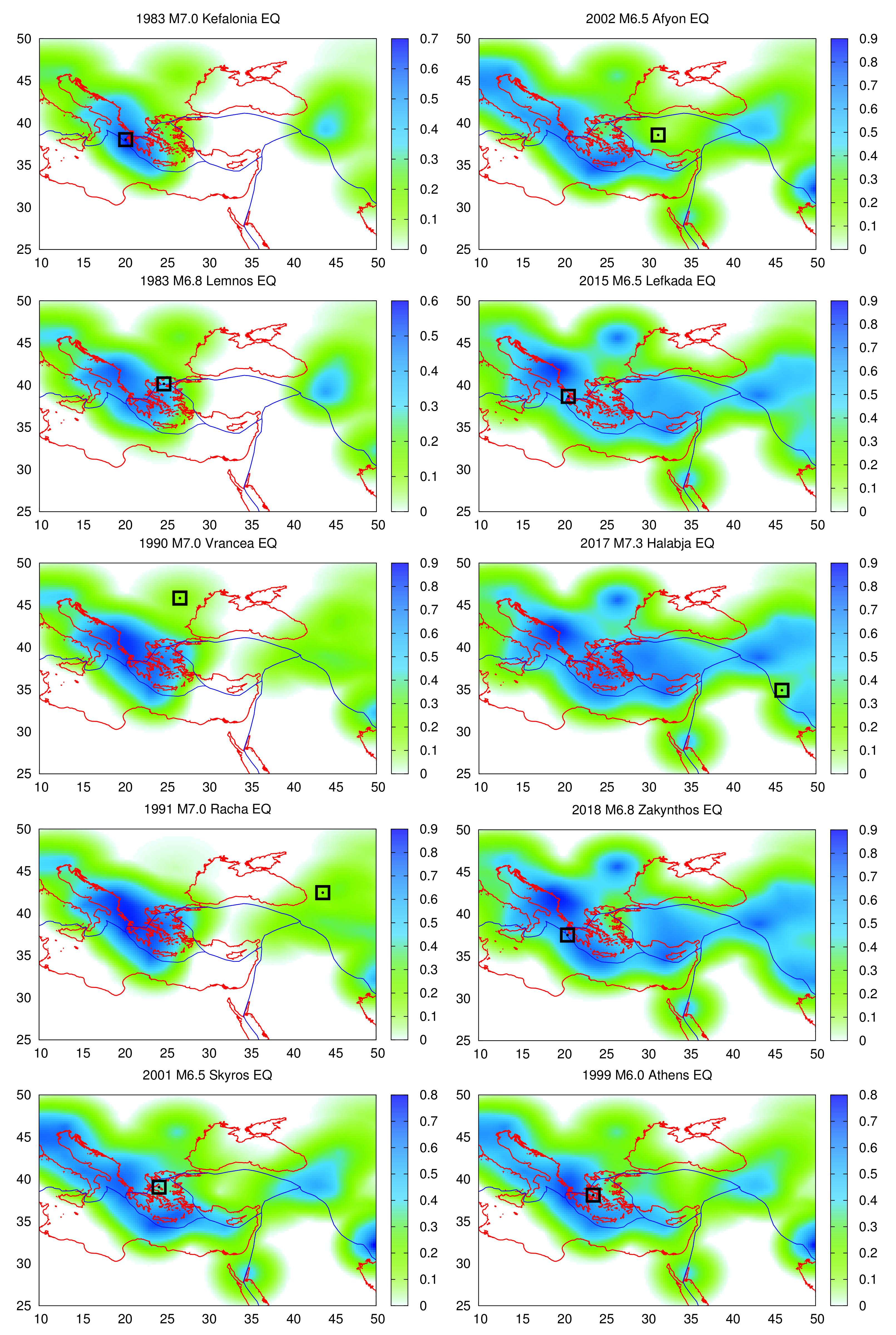
22 June 1982	17 January 1983	7.0	Kefalonia, Greece	64
21 June 1983	6 August 1983	6.8	Lemnos, Greece	32
3 April 1990	30 May 1990	7.0	Vrancea, Romania	20
11 November 1990	29 April 1991	7.0	Racha, Georgia	21
9 April 2001	26 July 2001	6.5	Skyros, Greece	36
21 January 2002	3 February 2002	6.5	Afyon, Turkey	10
15 April 2015	17 November 2015	6.5	Lefkada, Greece	55
12 June 2017	12 November 2017	7.3	Halabja, Iraq	31
24 April 2018	25 October 2018	6.8	Zakynthos, Greece	71
3 September 1999	7 September 1999	6.0	Athens, Greece	53

^a These data came from a compilation of Tables 2 and 3 of [115].

, and were used for the construction of the 〈EPS〉 maps shown in Figure 6. Figure 6 was drawn by using a 0.25${}^{\circ }\times 0.{25}^{\circ }$ grid as in Figure 4. In the last column of Table 2, the 〈EPS〉 estimated at the grid points nearest to the impending EQ epicenter are shown (cf. they had an average value 38% and an STD of 20%). A similar calculation revealed an average of 38% and an STD of 18% when a grid 0.1${}^{\circ }\times 0.1^{\circ }$ was used, pointing to the stability of the calculation.

Of course, the present method is a long way from becoming a really practical one, and we are still in the progress of improving it, since the cover of areas in Figure 4 and Figure 6 was too large to find the final epicenter of an impending strong EQ. It provides, however, insight to the very difficult question of forecasting strong EQs. At this point, it is worthwhile to add that, in the case of Japan, where better quality seismological data exist, we could obtain a better estimation of a future EQ epicenter location by means of an NTA [31,32].

The two cases of the local minima during September 1999, which corresponded to the last row of Table 1 and the last row of Table 2, concerning Düzce and Athens EQs, respectively, were of particular regional interest. These two minima were not reported before, as they corresponded to values ${\beta }_{80}$ and ${\beta }_{120}$, which were both well above 0.253. Their existence as local minima could be verified in Figure 2, while the corresponding 〈EPS〉 maps shown in Figure 4 and Figure 6 correlate well with the epicenters of the deadly EQs of Düzce and Athens in 1999. Interestingly, the minimum of ${\beta }_{80}$ on 3 September 1999 roughly coincided with the observation of an SES activity near Lamia, Greece, which was related to the deadly Athens EQ; see Chapter 17 of Lazaridou-Varotsos [142] (see also p. 105 of Reference [90]).

Moreover, a close inspection of Figure 2 revealed that local minima of ${\beta }_{80}$ in area $A_6$ coincided with the SES activities recorded on 17 March 2001 [143], 7 November 2007 [144], and 2 October 2018 [136]. These results were remarkable, as they provided additional evidence to support the conclusion [83] that SES activities were accompanied by clear variations of seismicity, giving rise to simultaneous precursory phenomena in independent geophysical observables. This behavior was, of course, more obvious in the case of mega-EQs such as the 2011 M9.0 Tohoku EQ in Japan. In particular, it was found that the deepest minimum ${\beta }_{min}$ of the order parameter ${\kappa }_1$ of seismicity during the 27-year period from 1 January 1984 to the occurrence of the 2011 Tohoku EQ occurrence on 11 March 2011 was observed on 5 January 2011 [29], which agreed with the experimental finding that ${\beta }_{min}$ was observed [83] when an SES activity was initiated. This was so because the date of 5 January 2011 overlapped with the observation [145,146,147] of the abnormal magnetic field variations on the z-component from 4 to 10 January 2011 at two measuring sites—see Figure 1 of [148]—laying at epicentral distances of around 130 km, a fact which was characteristic of the existence of an SES activity [4].

5. Conclusions

Here, we showed that upon computing maps of the average earthquake potential score in a self-consistent manner, we could obtain information on the epicenter location of an impending strong EQ. This was achieved by employing earthquake nowcasting at the time of the observation of the minimum ${\beta }_{min}$ of the fluctuations of the order parameter of seismicity. Such a minimum almost coincided with the SES activities, which were characterized by the development of long-range correlations, and became more easily detectable when a natural time analysis was employed in the areas covered by the higher order cores of the EQ networks based on similar activity patterns.

References

- Varotsos, P.A.; Sarlis, N.V.; Skordas, E.S. Spatio-Temporal complexity aspects on the interrelation between Seismic Electric Signals and Seismicity. Pract. Athens Acad. 2001, 76, 294–321. [Google Scholar]
- Varotsos, P.A.; Sarlis, N.V.; Skordas, E.S. Long-range correlations in the electric signals that precede rupture. Phys. Rev. E 2002, 66, 011902. [Google Scholar] [CrossRef] [PubMed] [Green Version]
- Varotsos, P.A.; Sarlis, N.V.; Skordas, E.S. Seismic Electric Signals and Seismicity: On a tentative interrelation between their spectral content. Acta Geophys. Pol. 2002, 50, 337–354. [Google Scholar]
- Varotsos, P.A.; Sarlis, N.V.; Skordas, E.S. Natural Time Analysis: The New View of Time. Precursory Seismic Electric Signals, Earthquakes and Other Complex Time-Series; Springer: Berlin/Heidelberg, Germany, 2011. [Google Scholar] [CrossRef]
- Varotsos, P.A.; Sarlis, N.V.; Skordas, E.S. Long-range correlations in the electric signals the precede rupture: Further investigations. Phys. Rev. E 2003, 67, 021109. [Google Scholar] [CrossRef] [Green Version]
- Varotsos, P.A.; Sarlis, N.V.; Skordas, E.S.; Uyeda, S.; Kamogawa, M. Natural time analysis of critical phenomena. Proc. Natl. Acad. Sci. USA 2011, 108, 11361–11364. [Google Scholar] [CrossRef] [Green Version]
- Sarlis, N.V.; Skordas, E.S.; Varotsos, P.A. Similarity of fluctuations in systems exhibiting Self-Organized Criticality. EPL (Europhys. Lett.) 2011, 96, 28006. [Google Scholar] [CrossRef]
- Sarlis, N.V.; Skordas, E.S.; Varotsos, P.A. The change of the entropy in natural time under time-reversal in the Olami-Feder-Christensen earthquake model. Tectonophysics 2011, 513, 49–53. [Google Scholar] [CrossRef]
- Sarlis, N.V.; Varotsos, P.A.; Skordas, E.S. Flux avalanches in YBa2Cu3O7-x films and rice piles: Natural time domain analysis. Phys. Rev. B 2006, 73, 054504. [Google Scholar] [CrossRef]
- Vallianatos, F.; Michas, G.; Benson, P.; Sammonds, P. Natural time analysis of critical phenomena: The case of acoustic emissions in triaxially deformed Etna basalt. Physica A 2013, 392, 5172–5178. [Google Scholar] [CrossRef]
- Varotsos, C.A.; Tzanis, C. A new tool for the study of the ozone hole dynamics over Antarctica. Atmos. Environ. 2012, 47, 428–434. [Google Scholar] [CrossRef]
- Varotsos, C.A.; Tzanis, C.; Cracknell, A.P. Precursory signals of the major El Niño Southern Oscillation events. Theor. Appl. Climatol. 2016, 124, 903–912. [Google Scholar] [CrossRef]
- Varotsos, C.A.; Tzanis, C.G.; Sarlis, N.V. On the progress of the 2015–2016 El Niño event. Atmos. Chem. Phys. 2016, 16, 2007–2011. [Google Scholar] [CrossRef] [Green Version]
- Varotsos, P.A.; Sarlis, N.V.; Skordas, E.S.; Lazaridou, M.S. Identifying sudden cardiac death risk and specifying its occurrence time by analyzing electrocardiograms in natural time. Appl. Phys. Lett. 2007, 91, 064106. [Google Scholar] [CrossRef]
- Sarlis, N.V.; Skordas, E.S.; Varotsos, P.A. Heart rate variability in natural time and 1/f “noise”. EPL 2009, 87, 18003. [Google Scholar] [CrossRef]
- Sarlis, N.V.; Christopoulos, S.R.G.; Bemplidaki, M.M. Change ΔS of the entropy in natural time under time reversal: Complexity measures upon change of scale. EPL 2015, 109, 18002. [Google Scholar] [CrossRef] [Green Version]
- Baldoumas, G.; Peschos, D.; Tatsis, G.; Chronopoulos, S.K.; Christofilakis, V.; Kostarakis, P.; Varotsos, P.; Sarlis, N.V.; Skordas, E.S.; Bechlioulis, A.; et al. A Prototype Photoplethysmography Electronic Device that Distinguishes Congestive Heart Failure from Healthy Individuals by Applying Natural Time Analysis. Electronics 2019, 8, 1288. [Google Scholar] [CrossRef] [Green Version]
- Baldoumas, G.; Peschos, D.; Tatsis, G.; Christofilakis, V.; Chronopoulos, S.K.; Kostarakis, P.; Varotsos, P.A.; Sarlis, N.V.; Skordas, E.S.; Bechlioulis, A.; et al. Remote sensing natural time analysis of heartbeat data by means of a portable photoplethysmography device. Int. J. Remote Sens. 2021, 42, 2292–2302. [Google Scholar] [CrossRef]
- Niccolini, G.; Manuello, A.; Marchis, E.; Carpinteri, A. Signal frequency distribution and natural-time analyses from acoustic emission monitoring of an arched structure in the Castle of Racconigi. Nat. Hazards Earth Syst. Sci. 2017, 17, 1025–1032. [Google Scholar] [CrossRef] [Green Version]
- Loukidis, A.; Pasiou, E.D.; Sarlis, N.V.; Triantis, D. Fracture analysis of typical construction materials in natural time. Physica A 2019, 547, 123831. [Google Scholar] [CrossRef]
- Loukidis, A.; Perez-Oregon, J.; Pasiou, E.D.; Sarlis, N.V.; Triantis, D. Similarity of fluctuations in critical systems: Acoustic emissions observed before fracture. Physica A 2020, 566, 125622. [Google Scholar] [CrossRef]
- Tanaka, H.K.; Varotsos, P.A.; Sarlis, N.V.; Skordas, E.S. A plausible universal behaviour of earthquakes in the natural time-domain. Proc. Jpn. Acad. Ser. B Phys. Biol. Sci. 2004, 80, 283–289. [Google Scholar] [CrossRef] [Green Version]
- Varotsos, P.A.; Sarlis, N.V.; Tanaka, H.K.; Skordas, E.S. Similarity of fluctuations in correlated systems: The case of seismicity. Phys. Rev. E 2005, 72, 041103. [Google Scholar] [CrossRef] [PubMed] [Green Version]
- Varotsos, P.A.; Sarlis, N.V.; Skordas, E.S.; Tanaka, H.K.; Lazaridou, M.S. Entropy of seismic electric signals: Analysis in the natural time under time reversal. Phys. Rev. E 2006, 73, 031114. [Google Scholar] [CrossRef] [PubMed] [Green Version]
- Varotsos, P.A.; Sarlis, N.V.; Skordas, E.S.; Tanaka, H.K.; Lazaridou, M.S. Attempt to distinguish long-range temporal correlations from the statistics of the increments by natural time analysis. Phys. Rev. E 2006, 74, 021123. [Google Scholar] [CrossRef]
- Varotsos, P.A.; Sarlis, N.V.; Skordas, E.S.; Lazaridou, M.S. Fluctuations, under time reversal, of the natural time and the entropy distinguish similar looking electric signals of different dynamics. J. Appl. Phys. 2008, 103, 014906. [Google Scholar] [CrossRef] [Green Version]
- Sarlis, N.V.; Skordas, E.S.; Varotsos, P.A. Multiplicative cascades and seismicity in natural time. Phys. Rev. E 2009, 80, 022102. [Google Scholar] [CrossRef] [Green Version]
- Sarlis, N.V.; Christopoulos, S.R.G. Natural time analysis of the Centennial Earthquake Catalog. Chaos 2012, 22, 023123. [Google Scholar] [CrossRef]
- Sarlis, N.V.; Skordas, E.S.; Varotsos, P.A.; Nagao, T.; Kamogawa, M.; Tanaka, H.; Uyeda, S. Minimum of the order parameter fluctuations of seismicity before major earthquakes in Japan. Proc. Natl. Acad. Sci. USA 2013, 110, 13734–13738. [Google Scholar] [CrossRef] [Green Version]
- Vallianatos, F.; Michas, G.; Papadakis, G. Non-extensive and natural time analysis of seismicity before the Mw6.4, October 12, 2013 earthquake in the South West segment of the Hellenic Arc. Physica A 2014, 414, 163–173. [Google Scholar] [CrossRef]
- Sarlis, N.V.; Skordas, E.S.; Varotsos, P.A.; Nagao, T.; Kamogawa, M.; Uyeda, S. Spatiotemporal variations of seismicity before major earthquakes in the Japanese area and their relation with the epicentral locations. Proc. Natl. Acad. Sci. USA 2015, 112, 986–989. [Google Scholar] [CrossRef] [Green Version]
- Huang, Q. Forecasting the epicenter of a future major earthquake. Proc. Natl. Acad. Sci. USA 2015, 112, 944–945. [Google Scholar] [CrossRef] [Green Version]
- Rundle, J.B.; Turcotte, D.L.; Donnellan, A.; Grant Ludwig, L.; Luginbuhl, M.; Gong, G. Nowcasting earthquakes. Earth Space Sci. 2016, 3, 480–486. [Google Scholar] [CrossRef]
- Potirakis, S.M.; Eftaxias, K.; Schekotov, A.; Yamaguchi, H.; Hayakawa, M. Criticality features in ultra-low frequency magnetic fields prior to the 2013 M6.3 Kobe earthquake. Ann. Geophys. 2016, 59, S0317. [Google Scholar] [CrossRef]
- Christopoulos, S.R.G.; Sarlis, N.V. An Application of the Coherent Noise Model for the Prediction of Aftershock Magnitude Time Series. Complexity 2017, 2017, 6853892. [Google Scholar] [CrossRef]
- Potirakis, S.M.; Asano, T.; Hayakawa, M. Criticality Analysis of the Lower Ionosphere Perturbations Prior to the 2016 Kumamoto (Japan) Earthquakes as Based on VLF Electromagnetic Wave Propagation Data Observed at Multiple Stations. Entropy 2018, 20, 199. [Google Scholar] [CrossRef] [Green Version]
- Sarlis, N.V.; Skordas, E.S.; Varotsos, P.A. A remarkable change of the entropy of seismicity in natural time under time reversal before the super-giant M9 Tohoku earthquake on 11 March 2011. EPL (Europhys. Lett.) 2018, 124, 29001. [Google Scholar] [CrossRef]
- Sarlis, N.V.; Skordas, E.S.; Varotsos, P.A.; Ramírez-Rojas, A.; Flores-Márquez, E.L. Natural time analysis: On the deadly Mexico M8.2 earthquake on 7 September 2017. Physica A 2018, 506, 625–634. [Google Scholar] [CrossRef]
- Varotsos, P.A.; Sarlis, N.V.; Skordas, E.S. Natural time analysis: Important changes of the order parameter of seismicity preceding the 2011 M9 Tohoku earthquake in Japan. EPL (Europhys. Lett.) 2019, 125, 69001. [Google Scholar] [CrossRef] [Green Version]
- Skordas, E.S.; Christopoulos, S.R.G.; Sarlis, N.V. Detrended fluctuation analysis of seismicity and order parameter fluctuations before the M7.1 Ridgecrest earthquake. Nat. Hazards 2020, 100, 697–711. [Google Scholar] [CrossRef]
- Sarlis, N.V.; Skordas, E.S.; Christopoulos, S.R.G.; Varotsos, P.A. Natural Time Analysis: The Area under the Receiver Operating Characteristic Curve of the Order Parameter Fluctuations Minima Preceding Major Earthquakes. Entropy 2020, 22, 583. [Google Scholar] [CrossRef]
- Yang, S.S.; Potirakis, S.M.; Sasmal, S.; Hayakawa, M. Natural Time Analysis of Global Navigation Satellite System Surface Deformation: The Case of the 2016 Kumamoto Earthquakes. Entropy 2020, 22, 674. [Google Scholar] [CrossRef]
- Varotsos, P.A.; Skordas, E.S.; Sarlis, N.V. Fluctuations of the entropy change under time reversal: Further investigations on identifying the occurrence time of an impending major earthquake. EPL (Europhys. Lett.) 2020, 130, 29001. [Google Scholar] [CrossRef]
- Varotsos, P.A.; Sarlis, N.V.; Skordas, E.S. Self-organized criticality and earthquake predictability: A long-standing question in the light of natural time analysis. EPL (Europhys. Lett.) 2020, 132, 29001. [Google Scholar] [CrossRef]
- Vallianatos, F.; Michas, G.; Hloupis, G. Seismicity Patterns Prior to the Thessaly (Mw6.3) Strong Earthquake on 3 March 2021 in Terms of Multiresolution Wavelets and Natural Time Analysis. Geosciences 2021, 11, 379. [Google Scholar] [CrossRef]
- Bak, P.; Christensen, K.; Danon, L.; Scanlon, T. Unified Scaling Law for Earthquakes. Phys. Rev. Lett. 2002, 88, 178501. [Google Scholar] [CrossRef] [Green Version]
- Baiesi, M.; Paczuski, M. Scale-free networks of earthquakes and aftershocks. Phys. Rev. E 2004, 69, 066106. [Google Scholar] [CrossRef] [Green Version]
- Davidsen, J.; Paczuski, M. Analysis of the Spatial Distribution Between Successive Earthquakes. Phys. Rev. Lett. 2005, 94, 048501. [Google Scholar] [CrossRef] [Green Version]
- Corral, A. Long-Term Clustering, Scaling, and Universality in the Temporal Occurrence of Earthquakes. Phys. Rev. Lett. 2004, 92, 108501. [Google Scholar] [CrossRef] [Green Version]
- Saichev, A.; Sornette, D. Vere-Jones’ self-similar branching model. Phys. Rev. E 2005, 72, 056122. [Google Scholar] [CrossRef] [Green Version]
- Livina, V.N.; Havlin, S.; Bunde, A. Memory in the Occurrence of Earthquakes. Phys. Rev. Lett. 2005, 95, 208501. [Google Scholar] [CrossRef] [Green Version]
- Eichner, J.F.; Kantelhardt, J.W.; Bunde, A.; Havlin, S. Statistics of return intervals in long-term correlated records. Phys. Rev. E 2007, 75, 011128. [Google Scholar] [CrossRef] [PubMed] [Green Version]
- Lennartz, S.; Livina, V.N.; Bunde, A.; Havlin, S. Long-term memory in earthquakes and the distribution of interoccurrence times. EPL (Europhys. Lett.) 2008, 81, 69001. [Google Scholar] [CrossRef] [Green Version]
- Huang, Q. Seismicity changes prior to the Ms8.0 Wenchuan earthquake in Sichuan, China. Geophys. Res. Lett. 2008, 35, L23308. [Google Scholar] [CrossRef]
- Lennartz, S.; Bunde, A.; Turcotte, D.L. Modelling seismic catalogues by cascade models: Do we need long-term magnitude correlations? Geophys. J. Int. 2011, 184, 1214–1222. [Google Scholar] [CrossRef] [Green Version]
- Huang, Q. Retrospective investigation of geophysical data possibly associated with the Ms8.0 Wenchuan earthquake in Sichuan, China. J. Asian Earth Sci. 2011, 41, 421–427. [Google Scholar] [CrossRef]
- Zaliapin, I.; Gabrielov, A.; Keilis-Borok, V.; Wong, H. Clustering analysis of seismicity and aftershock identification. Phys. Rev. Lett. 2008, 101, 018501. [Google Scholar] [CrossRef] [Green Version]
- Tiampo, K.F.; Rundle, J.B.; Klein, W.; Holliday, J.; Sá Martins, J.S.; Ferguson, C.D. Ergodicity in natural earthquake fault networks. Phys. Rev. E 2007, 75, 066107. [Google Scholar] [CrossRef] [Green Version]
- Lippiello, E.; Godano, C.; de Arcangelis, L. Dynamical Scaling in Branching Models for Seismicity. Phys. Rev. Lett. 2007, 98, 098501. [Google Scholar] [CrossRef] [Green Version]
- Tenenbaum, J.N.; Havlin, S.; Stanley, H.E. Earthquake networks based on similar activity patterns. Phys. Rev. E 2012, 86, 046107. [Google Scholar] [CrossRef] [Green Version]
- Lippiello, E.; Godano, C.; de Arcangelis, L. The earthquake magnitude is influenced by previous seismicity. Geophys. Res. Lett. 2012, 39, L05309. [Google Scholar] [CrossRef]
- Huang, Q.; Ding, X. Spatiotemporal variations of seismic quiescence prior to the 2011 M 9.0 Tohoku earthquake revealed by an improved region-time-length algorithm. Bull. Seismol. Soc. Am. 2012, 102, 1878–1883. [Google Scholar] [CrossRef]
- Bunde, A.; Lennartz, S. Long-Term Correlations in Earth Sciences. Acta Geophys. 2012, 60, 562–588. [Google Scholar] [CrossRef]
- Tiampo, K.F.; Shcherbakov, R. Seismicity-based earthquake forecasting techniques: Ten years of progress. Tectonophysics 2012, 522–523, 89–121. [Google Scholar] [CrossRef]
- Zaliapin, I.; Ben-Zion, Y. Earthquake clusters in southern California I: Identification and stability. J. Geophys. Res. Solid Earth 2013, 118, 2847–2864. [Google Scholar] [CrossRef]
- Zaliapin, I.; Ben-Zion, Y. Earthquake clusters in southern California II: Classification and relation to physical properties of the crust. J. Geophys. Res. Solid Earth 2013, 118, 2865–2877. [Google Scholar] [CrossRef]
- Batac, R.C.; Kantz, H. Observing spatio-temporal clustering and separation using interevent distributions of regional earthquakes. Nonlin. Processes Geophys. 2014, 21, 735–744. [Google Scholar] [CrossRef]
- Zaliapin, I.; Ben-Zion, Y. Artefacts of earthquake location errors and short-term incompleteness on seismicity clusters in southern California. Geophys. J. Int. 2015, 202, 1949–1968. [Google Scholar] [CrossRef] [Green Version]
- de Arcangelis, L.; Godano, C.; Grasso, J.R.; Lippiello, E. Statistical physics approach to earthquake occurrence and forecasting. Phys. Rep. 2016, 628, 1–91. [Google Scholar] [CrossRef]
- Turcotte, D.L. Fractals and Chaos in Geology and Geophysics, 2nd ed.; Cambridge University Press: Cambridge, UK, 1997. [Google Scholar] [CrossRef]
- Scholz, C.H. The mechanics of Earthquakes and Faulting, 2nd ed.; Cambridge University Press: Cambridge, UK, 2002. [Google Scholar] [CrossRef]
- Holliday, J.R.; Rundle, J.B.; Turcotte, D.L.; Klein, W.; Tiampo, K.F.; Donnellan, A. Space-Time Clustering and Correlations of Major Earthquakes. Phys. Rev. Lett. 2006, 97, 238501. [Google Scholar] [CrossRef] [Green Version]
- Sornette, D. Critical Phenomena in the Natural Sciences: Chaos, Fractals, Selforganization, and Disorder: Concepts and Tools; Springer: Berlin/Heidelberg, Germany, 2000. [Google Scholar] [CrossRef]
- Carlson, J.M.; Langer, J.S.; Shaw, B.E. Dynamics of earthquake faults. Rev. Mod. Phys. 1994, 66, 657–670. [Google Scholar] [CrossRef]
- Xia, J.; Gould, H.; Klein, W.; Rundle, J.B. Near-mean-field behavior in the generalized Burridge-Knopoff earthquake model with variable-range stress transfer. Phys. Rev. E 2008, 77, 031132. [Google Scholar] [CrossRef] [Green Version]
- Rundle, J.B.; Klein, W.; Gross, S. Dynamics of a Traveling Density Wave Model for Earthquakes. Phys. Rev. Lett. 1996, 76, 4285–4288. [Google Scholar] [CrossRef]
- Fisher, D.S.; Dahmen, K.; Ramanathan, S.; Ben-Zion, Y. Statistics of Earthquakes in Simple Models of Heterogeneous Faults. Phys. Rev. Lett. 1997, 78, 4885–4888. [Google Scholar] [CrossRef] [Green Version]
- Rundle, J.B.; Turcotte, D.L.; Shcherbakov, R.; Klein, W.; Sammis, C. Statistical physics approach to understanding the multiscale dynamics of earthquake fault systems. Rev. Geophys. 2003, 41, 1019. [Google Scholar] [CrossRef] [Green Version]
- Landau, L.D.; Lifshitz, E.M. Statistical Physics, 3nd ed.; Pergamon Press: Oxford, UK, 1980. [Google Scholar]
- Flores-Márquez, E.L.; Ramírez-Rojas, A.; Perez-Oregon, J.; Sarlis, N.V.; Skordas, E.S.; Varotsos, P.A. Natural Time Analysis of Seismicity within the Mexican Flat Slab before the M7.1 Earthquake on 19 September 2017. Entropy 2020, 22, 730. [Google Scholar] [CrossRef]
- Varotsos, P.A.; Sarlis, N.V.; Skordas, E.S. Remarkable changes in the distribution of the order parameter of seismicity before mainshocks. EPL 2012, 100, 39002. [Google Scholar] [CrossRef] [Green Version]
- Varotsos, P.A.; Sarlis, N.V.; Skordas, E.S. Scale-specific order parameter fluctuations of seismicity in natural time before mainshocks. EPL 2011, 96, 59002. [Google Scholar] [CrossRef] [Green Version]
- Varotsos, P.A.; Sarlis, N.V.; Skordas, E.S.; Lazaridou, M.S. Seismic Electric Signals: An additional fact showing their physical interconnection with seismicity. Tectonophysics 2013, 589, 116–125. [Google Scholar] [CrossRef]
- Varotsos, P.; Alexopoulos, K.; Nomicos, K. Seismic Electric Currents. Pract. Athens Acad. 1981, 56, 277–286. [Google Scholar]
- Varotsos, P.; Alexopoulos, K. Physical Properties of the variations of the electric field of the Earth preceding earthquakes, I. Tectonophysics 1984, 110, 73–98. [Google Scholar] [CrossRef]
- Varotsos, P.; Alexopoulos, K. Physical Properties of the variations of the electric field of the Earth preceding earthquakes, II. Tectonophysics 1984, 110, 99–125. [Google Scholar] [CrossRef]
- Varotsos, P.; Alexopoulos, K. Thermodynamics of Point Defects and their Relation with Bulk Properties; North Holland: Amsterdam, The Netherlands, 1986. [Google Scholar]
- Varotsos, P.; Lazaridou, M. Latest aspects of earthquake prediction in Greece based on Seismic Electric Signals. Tectonophysics 1991, 188, 321–347. [Google Scholar] [CrossRef]
- Varotsos, P.; Alexopoulos, K.; Lazaridou, M. Latest aspects of earthquake prediction in Greece based on Seismic Electric Signals, II. Tectonophysics 1993, 224, 1–37. [Google Scholar] [CrossRef] [Green Version]
- Varotsos, P. The Physics of Seismic Electric Signals; TERRAPUB: Tokyo, Japan, 2005; p. 338. [Google Scholar]
- Sarlis, N.V.; Christopoulos, S.R.G.; Skordas, E.S. Minima of the fluctuations of the order parameter of global seismicity. Chaos 2015, 25, 063110. [Google Scholar] [CrossRef] [Green Version]
- Sarlis, N.V.; Skordas, E.S.; Christopoulos, S.R.G.; Varotsos, P.A. Statistical Significance of Minimum of the Order Parameter Fluctuations of Seismicity Before Major Earthquakes in Japan. Pure Appl. Geophys. 2016, 173, 165–172. [Google Scholar] [CrossRef] [Green Version]
- Sarlis, N.V.; Skordas, E.S.; Mintzelas, A.; Papadopoulou, K.A. Micro-scale, mid-scale, and macro-scale in global seismicity identified by empirical mode decomposition and their multifractal characteristics. Sci. Rep. 2018, 8, 9206. [Google Scholar] [CrossRef]
- Christopoulos, S.R.G.; Skordas, E.S.; Sarlis, N.V. On the Statistical Significance of the Variability Minima of the Order Parameter of Seismicity by Means of Event Coincidence Analysis. Appl. Sci. 2020, 10, 662. [Google Scholar] [CrossRef] [Green Version]
- Varotsos, P.A.; Sarlis, N.V.; Skordas, E.S. Study of the temporal correlations in the magnitude time series before major earthquakes in Japan. J. Geophys. Res. Space Phys. 2014, 119, 9192–9206. [Google Scholar] [CrossRef]
- Sarlis, N.V.; Skordas, E.S.; Varotsos, P.A.; Ramírez-Rojas, A.; Flores-Márquez, E.L. Identifying the Occurrence Time of the Deadly Mexico M8.2 Earthquake on 7 September 2017. Entropy 2019, 21, 301. [Google Scholar] [CrossRef] [Green Version]
- Watts, D.J.; Strogatz, S.H. Collective dynamics of ‘small-world’ networks. Nature 1998, 393, 440–442. [Google Scholar] [CrossRef]
- Albert, R.; Barabási, A.L. Statistical mechanics of complex networks. Rev. Mod. Phys. 2002, 74, 47–97. [Google Scholar] [CrossRef] [Green Version]
- Dorogovtsev, S.N.; Goltsev, A.V.; Mendes, J.F.F. Critical phenomena in complex networks. Rev. Mod. Phys. 2008, 80, 1275–1335. [Google Scholar] [CrossRef] [Green Version]
- Newman, M.E.J. Networks: An Introduction; Oxford University Press: Oxford, UK, 2010. [Google Scholar] [CrossRef] [Green Version]
- Di Muro, M.A.; La Rocca, C.E.; Stanley, H.E.; Havlin, S.; Braunstein, L.A. Recovery of Interdependent Networks. Sci. Rep. 2016, 6, 22834. [Google Scholar] [CrossRef]
- Baiesi, M.; Paczuski, M. Complex networks of earthquakes and aftershocks. Nonlin. Processes Geophys. 2005, 12, 1–11. [Google Scholar] [CrossRef]
- Baiesi, M. Scaling and precursor motifs in earthquake networks. Physica A 2006, 360, 534–542. [Google Scholar] [CrossRef] [Green Version]
- Davidsen, J.; Grassberger, P.; Paczuski, M. Networks of recurrent events, a theory of records, and an application to finding causal signatures in seismicity. Phys. Rev. E 2008, 77, 066104. [Google Scholar] [CrossRef] [Green Version]
- Krishna Mohan, T.R.; Revathi, P.G. Earthquake correlations and networks: A comparative study. Phys. Rev. E 2011, 83, 046109. [Google Scholar] [CrossRef] [Green Version]
- Telesca, L.; Lovallo, M. Analysis of seismic sequences by using the method of visibility graph. EPL (Europhys. Lett.) 2012, 97, 50002. [Google Scholar] [CrossRef]
- Telesca, L.; Lovallo, M.; Ramirez-Rojas, A.; Flores-Marquez, L. Investigating the time dynamics of seismicity by using the visibility graph approach: Application to seismicity of Mexican subduction zone. Physica A 2013, 392, 6571–6577. [Google Scholar] [CrossRef]
- Telesca, L.; Lovallo, M.; Ramirez-Rojas, A.; Flores-Marquez, L. Relationship between the Frequency Magnitude Distribution and the Visibility Graph in the Synthetic Seismicity Generated by a Simple Stick-Slip System with Asperities. PLoS ONE 2014, 9, e106233. [Google Scholar] [CrossRef] [Green Version]
- Telesca, L.; Lovallo, M.; Aggarwal, S.; Khan, P. Precursory signatures in the visibility graph analysis of seismicity: An application to the Kachchh (Western India) seismicity. Phys. Chem. Earth 2015, 85-86, 195–200. [Google Scholar] [CrossRef]
- Telesca, L.; Lovallo, M.; Aggarwal, S.K.; Khan, P.K.; Rastogi, B.K. Visibility Graph Analysis of the 2003–2012 Earthquake Sequence in the Kachchh Region of Western India. Pure Appl. Geophys. 2016, 173, 125–132. [Google Scholar] [CrossRef]
- Telesca, L.; Cheldize, T. Visibility graph analysis of seismicity around Enguri high arch dam, Caucasus. Bull. Seismol. Soc. Am. 2018, 108, 3141–3147. [Google Scholar] [CrossRef]
- Chorozoglou, D.; Kugiumtzis, D.; Papadimitriou, E. Application of complex network theory to the recent foreshock sequences of Methoni (2008) and Kefalonia (2014) in Greece. Acta Geophys. 2017, 65, 543–553. [Google Scholar] [CrossRef]
- Chorozoglou, D.; Kugiumtzis, D.; Papadimitriou, E. Testing the structure of earthquake networks from multivariate time series of successive main shocks in Greece. Physica A 2018, 499, 28–39. [Google Scholar] [CrossRef]
- Chorozoglou, D.; Papadimitriou, E.; Kugiumtzis, D. Investigating small-world and scale-free structure of earthquake networks in Greece. Chaos Solitons Fractals 2019, 122, 143–152. [Google Scholar] [CrossRef]
- Mintzelas, A.; Sarlis, N. Minima of the fluctuations of the order parameter of seismicity and earthquake networks based on similar activity patterns. Physica A 2019, 527, 121293. [Google Scholar] [CrossRef]
- Pasari, S. Nowcasting Earthquakes in the Bay of Bengal Region. Pure Appl. Geophys. 2019, 176, 1417–1432. [Google Scholar] [CrossRef]
- Rundle, J.B.; Luginbuhl, M.; Giguere, A.; Turcotte, D.L. Natural Time, Nowcasting and the Physics of Earthquakes: Estimation of Seismic Risk to Global Megacities. Pure Appl. Geophys. 2018, 175, 647–660. [Google Scholar] [CrossRef] [Green Version]
- Luginbuhl, M.; Rundle, J.B.; Hawkins, A.; Turcotte, D.L. Nowcasting Earthquakes: A Comparison of Induced Earthquakes in Oklahoma and at the Geysers, California. Pure Appl. Geophys. 2018, 175, 49–65. [Google Scholar] [CrossRef]
- Luginbuhl, M.; Rundle, J.B.; Turcotte, D.L. Natural Time and Nowcasting Earthquakes: Are Large Global Earthquakes Temporally Clustered? Pure Appl. Geophys. 2018, 175, 661–670. [Google Scholar] [CrossRef]
- Luginbuhl, M.; Rundle, J.B.; Turcotte, D.L. Natural time and nowcasting induced seismicity at the Groningen gas field in the Netherlands. Geophys. J. Int. 2018, 215, 753–759. [Google Scholar] [CrossRef]
- Rundle, J.B.; Luginbuhl, M.; Khapikova, P.; Turcotte, D.L.; Donnellan, A.; McKim, G. Nowcasting Great Global Earthquake and Tsunami Sources. Pure Appl. Geophys. 2020, 177, 359–368. [Google Scholar] [CrossRef]
- Rundle, J.B.; Giguere, A.; Turcotte, D.L.; Crutchfield, J.P.; Donnellan, A. Global Seismic Nowcasting With Shannon Information Entropy. Earth Space Sci. 2019, 6, 191–197. [Google Scholar] [CrossRef] [Green Version]
- Pasari, S.; Sharma, Y. Contemporary Earthquake Hazards in the West-Northwest Himalaya: A Statistical Perspective through Natural Times. Seismol. Res. Lett. 2020, 91, 3358–3369. [Google Scholar] [CrossRef]
- Perez-Oregon, J.; Muñoz Diosdado, A.; Rudolf-Navarro, A.H.; Angulo-Brown, F. A Simple Model to Relate the Elastic Ratio Gamma of a Critically Self-Organized Spring-Block Model with the Age of a Lithospheric Downgoing Plate in a Subduction Zone. Entropy 2020, 22, 868. [Google Scholar] [CrossRef]
- Rundle, J.B.; Donnellan, A.; Fox, G.; Crutchfield, J.P. Nowcasting Earthquakes by Visualizing the Earthquake Cycle with Machine Learning: A Comparison of Two Methods. Surv. Geophys. 2021, 1–19. [Google Scholar] [CrossRef]
- Rundle, J.B.; Donnellan, A.; Fox, G.; Crutchfield, J.P.; Granat, R. Nowcasting Earthquakes: Imaging the Earthquake Cycle in California with Machine Learning. Earth Space Sci. 2021, e2021EA001757. [Google Scholar] [CrossRef]
- United States Geological Survey, Earthquake Hazards Program. Search Earthquake Catalog. Available online: https://earthquake.usgs.gov/earthquakes/search/ (accessed on 9 February 2021).
- Taymaz, T.; Jackson, J.; McKenzie, D. Active tectonics of the north and central Aegean Sea. Geophys. J. Int. 1991, 106, 433–490. [Google Scholar] [CrossRef]
- Devoti, R.; Ferraro, C.; Gueguen, E.; Lanotte, R.; Luceri, V.; Nardi, A.; Pacione, R.; Rutigliano, P.; Sciarretta, C.; Vespe, F. Geodetic control on recent tectonic movements in the central Mediterranean area. Tectonophysics 2002, 346, 151–167. [Google Scholar] [CrossRef]
- Kassaras, I.; Kapetanidis, V.; Ganas, A.; Tzanis, A.; Kosma, C.; Karakonstantis, A.; Valkaniotis, S.; Chailas, S.; Kouskouna, V.; Papadimitriou, P. The New Seismotectonic Atlas of Greece (v1.0) and Its Implementation. Geosciences 2020, 10, 447. [Google Scholar] [CrossRef]
- McKenzie, D. Active tectonics of the Alpine—Himalayan belt: The Aegean Sea and surrounding regions. Geophys. J. Int. 1978, 55, 217–254. [Google Scholar] [CrossRef] [Green Version]
- Bird, P. An updated digital model of plate boundaries. Geochem. Geophys. Geosyst. 2003, 4, 1027. [Google Scholar] [CrossRef]
- Kanamori, H. Quantification of Earthquakes. Nature 1978, 271, 411–414. [Google Scholar] [CrossRef]
- Sarlis, N.V.; Skordas, E.S.; Varotsos, P.A. Order parameter fluctuations of seismicity in natural time before and after mainshocks. EPL 2010, 91, 59001. [Google Scholar] [CrossRef] [Green Version]
- Goldenfeld, N. Lectures on Phase Transitions and the Renormalization Group; CRC Press, Taylor & Francis Group: Boca Raton, FL, USA, 2018. [Google Scholar]
- Sarlis, N.V.; Skordas, E.S. Study in Natural Time of Geoelectric Field and Seismicity Changes Preceding the Mw6.8 Earthquake on 25 October 2018 in Greece. Entropy 2018, 20, 882. [Google Scholar] [CrossRef] [Green Version]
- Ferguson, C.D.; Klein, W.; Rundle, J.B. Spinodals, scaling, and ergodicity in a threshold model with long-range stress transfer. Phys. Rev. E 1999, 60, 1359–1373. [Google Scholar] [CrossRef]
- Tiampo, K.F.; Rundle, J.B.; Klein, W.; Martins, J.S.S.; Ferguson, C.D. Ergodic Dynamics in a Natural Threshold System. Phys. Rev. Lett. 2003, 91, 238501. [Google Scholar] [CrossRef] [Green Version]
- Press, W.H.; Teukolsky, S.; Vettrling, W.; Flannery, B.P. Numerical Recipes in FORTRAN; Cambridge Univrsity Press: New York, NY, USA, 1992; p. 963. [Google Scholar]
- Weisstein, E.W. Circle-Circle Intersection. From MathWorld—A Wolfram Web Resource. 2021. Available online: https://mathworld.wolfram.com/Circle-CircleIntersection.html (accessed on 15 September 2021).
- Sarlis, N.V.; Skordas, E.S.; Varotsos, P.A.; Ramírez-Rojas, A.; Flores-Márquez, E.L. Investigation of the temporal correlations between earthquake magnitudes before the Mexico M8.2 earthquake on 7 September 2017. Physica A 2019, 517, 475–483. [Google Scholar] [CrossRef]
- Lazaridou-Varotsos, M.S. Earthquake Prediction by Seismic Electric Signals: The success of the VAN method over thirty years; Springer Praxis Books: Berlin/Heidelberg, Germany, 2013. [Google Scholar]
- Varotsos, P.; Sarlis, N.; Skordas, E. A note on the spatial extent of the Volos SES sensitive site. Acta Geophys. Pol. 2001, 49, 425–435. [Google Scholar]
- Sarlis, N.V.; Skordas, E.S.; Lazaridou, M.S.; Varotsos, P.A. Investigation of seismicity after the initiation of a Seismic Electric Signal activity until the main shock. Proc. Jpn. Acad. Ser. B Phys. Biol. Sci. 2008, 84, 331–343. [Google Scholar] [CrossRef] [PubMed]
- Xu, G.; Han, P.; Huang, Q.; Hattori, K.; Febriani, F.; Yamaguchi, H. Anomalous behaviors of geomagnetic diurnal variations prior to the 2011 off the Pacific coast of Tohoku earthquake (Mw9.0). J. Asian Earth Sci. 2013, 77, 59–65. [Google Scholar] [CrossRef] [Green Version]
- Han, P.; Hattori, K.; Xu, G.; Ashida, R.; Chen, C.H.; Febriani, F.; Yamaguchi, H. Further investigations of geomagnetic diurnal variations associated with the 2011 off the Pacific coast of Tohoku earthquake (Mw 9.0). J. Asian Earth Sci. 2015, 114, 321–326. [Google Scholar] [CrossRef]
- Han, P.; Hattori, K.; Huang, Q.; Hirooka, S.; Yoshino, C. Spatiotemporal characteristics of the geomagnetic diurnal variation anomalies prior to the 2011 Tohoku earthquake (Mw 9.0) and the possible coupling of multiple pre-earthquake phenomena. J. Asian Earth Sci. 2016, 129, 13–21. [Google Scholar] [CrossRef]
- Skordas, E.S.; Sarlis, N.V.; Varotsos, P.A. Identifying the occurrence time of an impending major earthquake by means of the fluctuations of the entropy change under time reversal. EPL (Europhys. Lett.) 2019, 128, 49001. [Google Scholar] [CrossRef]
- Williams, T.; Kelley, C. Gnuplot 4.6: An Interactive Plotting Program. 2014. Available online: http://www.gnuplot.info (accessed on 28 February 2014).
- Metzger, D.R. GEODAS Coastline Extractor, Version 1.1.3.1. 2014. Available online: http://www.ngdc.noaa.gov/mgg/dat/geodas/software/mswindows/geodas-ng_setup.exe (accessed on 11 February 2015).