Abstract
Conducting physical attendance exams during pandemics is a challenge facing many educational institutes and universities. Our study’s main objective is to numerically simulate the expected transmission of the harmful exhaled droplets of aerosols from an infected instructor to students in an exam room ventilated by a number of spiral diffusers. Several critical parameters, including the droplet size, the ventilation rate, and status of the entrance door were considered in the analysis. Two dimensionless indices, i.e., the specific normalized average concentration (SNAC) and the exceedance in exposure ratio (EER), were introduced to examine the effect of the said parameters on student exposure to the harmful droplets. The study revealed that the 5 μm droplets were less hazardous as they resulted in an 87% reduction in exposure when compared with the small 1 μm size droplets. We also found that when the ventilation rate ratio (VRR) increased above unity, an upward entrainment process, due to the swirl diffuser, of the aerosol droplets took place, and consequently the risk of student exposure was reduced. The results also demonstrated that increasing VRR from zero to 1 and then to 2 decreased the exceedance in the student exposure from 3.5 to 2.15 and then to less than zero, respectively. The study also showed that keeping the lecture room’s main door open is recommended as this reduced the risk of exposure by 26% in the case of a VRR equal to 2.
1. Introduction
During the 2003 SARS outbreak, over 8000 people from more than 20 different countries were infected, and 774 died worldwide [1]. In 2009–2010, the swine flu pandemic lasted for about 19 months, where the WHO reported 18,500 laboratory-confirmed deaths. However, Dawood et al. estimated that, globally, about 284,000 (range from 150,000 to 575,000) deaths were caused by this pandemic [2]. Since 2012, the MERS-CoV outbreak has affected several countries worldwide but was concentrated mainly in the Middle East. Peck et al. reported in 2015 a total of 1227 confirmed human cases of MERS, resulting in 449 deaths [3].
In a few months since its appearance in 2019, the COVID-19 virus widely spread to all countries and became a worldwide crisis. The infection caused many countries to close their borders, suspend air flights, and force either extended lockdowns or semi-lockdowns on their residents. Almost all schools and colleges globally conducted virtual classes to prevent further spreading of the virus. Some countries ultimately canceled their schools’ exams, and most universities worldwide conducted online exams for both semesters in 2020. Despite these measures taken, the global infected cases of COVID-19 exceeded two hundred and twenty-four million, the reported deaths approached five million by the end of 2021, and these numbers are still increasing [4].
Several sources suggested that viruses attacking the respiratory system are transmitted by three routes: (1) large droplets from the infected person that are exhaled with enough momentum to directly impact the mouth, nose, or conjunctiva (eyes) of the recipients; (2) physical contact with infected droplets that are deposited on any surface and subsequently transmitted to the recipient’s respiratory mucosa by hand contact; and (3) inhalation by the recipient of infected nuclei (aerosol size droplets) delivered by ambient air currents. The first two routes are referred to as the “droplet” or “contact” routes of transmission, while the third is called the “airborne” transmission route [5,6,7,8,9,10,11,12,13,14,15]. Thus, safety measures should be applied to the airborne route.
One of these safety measures for mitigation is to keep sufficient social distance among people. Some researchers estimate that distance to be around 1.5 to 2 m [14]. It is assumed that this distance is feasible and practical, believing that the largest exhaled droplets will eventually settle by gravity or evaporate before moving this distance and affecting the other person. However, several studies have shown that exhaled droplets from breathing, coughing, and sneezing can sometimes travel up to 6 m and even further [16,17,18,19,20].
Several researchers have studied characterizations of exhaled air velocity, droplet size distributions, and their concentrations during different respiratory activities. However, only a few researchers measured these characters for exhaled air during speaking activities. Morawska et al. measured the size of droplets produced during speaking, where they found that the modes of droplet sizes were in the range of 3.5 to 5.5 µm, with corresponding average concentrations in the range of 0.04 and 0.16 particles per cubic cm (cm−3 or p/cm3), respectively. For the entire size range examined of 0.3–20 µm, the average particle concentration produced during speaking was 1.1 cm−3 [21].
Chao et al. measured an average expiration air velocity of approximately 4.6 m/s for men during speaking, where the geometric mean diameter of droplets was 16.0 µm and the mode was 6 µm. They estimated that droplet concentrations were in the range of 0.004–0.223 cm−3 for speaking [22]. Kwon et al. found that the average initial speaking velocity was 4.07 m/s for men [23]. In their review, Zhang et al. mentioned that the speaking droplet size ranged between 0.1 and 16 µm, while most researchers measured it below 8 µm, while the concentration of the droplets reached 1.2 cm−3 [24]. Recently, Liu et al. measured the peak concentration of COVID-19 aerosols to appear in two size ranges; the first range in the submicron region with a diameter between 0.25 to 1.0 μm, and the second peak in the supermicron region with a diameter larger than 2.5 μm [25].
CFD simulation of exhaled droplets, during transmission indoors, has been studied by several researchers [17,26,27,28,29,30,31,32,33,34,35,36,37,38,39]. Most of the studied cases describe the transfer of exhaled droplets from an infected person to others under different locations, conditions, and ventilation systems. The most studied places were hospital rooms, offices, and conference rooms. The main concern in most of those publications was investigating the transmission of infectious droplets from patients to others by calculating different variables, such as the velocity distribution, particle concentrations, and deposition under different ventilation conditions and different room geometries. In all these simulations, the infectious droplets were generated by the infected person by coughing, sneezing, or breathing.
The education sector is one of the most challenging sectors that requires flexible and careful strategies to deal with pandemic situations. Such plans should be based on a deep understanding of the airborne diseases and how they are expected to disperse in classrooms and exam hall environments.
2. Scope and Objectives
As per the best of the authors’ knowledge, only one study in early 2021, Shao et al. [40], investigated the case of speaking from an infected instructor. Shao et al. conducted experiments with an optical diagnosing technique. The integrated Schlieren imaging and digital inline holography systems were used to measure the exhaled gas flow field and the sizes/distribution of the generated particles through the normal breathing behavior of eight participants. They also conducted a CFD simulation (with coarse meshes of 80,000 and 160,000 grid points in a classroom 5 × 10 × 3 m) using the open-source OpenFOAM-6 CFD package to evaluate the risk of students inhaling from an infected instructor during speaking.
The current research work is considered a step forward in studying the safety of the students during exam time. This study attempts to simulate exhaled droplet dispersion from an infected instructor to students during exam time in a real classroom at Imam Mohammad Ibn Saud University, Riyadh, under different real ventilation scenarios. The authors do not attempt to give a complete solution to the problem but rather provide initial guidelines to the minimum ventilation requirements and the student distribution in the classroom to minimize the transmission of the airborne infection from the instructor to students. Due to the urgency of the current situation and the lack of research on the transmission of infectious diseases in classrooms, this work attempts to provide an essential overview of challenges and required measures supplemented with a potential practical framework.
The main objectives of the study in-hand are:
- To numerically track the spreading of the aerosol particles with time-based on a calibrated CFD model with decent spatial resolution.
- To introduce some well-defined dimensionless parameters that could be used to assess the vulnerability to the exposure of the droplets of aerosols.
- To investigate the effect of adopting different ventilation schemes on the students’ expected exposure to the aerosol droplets.
- To investigate the effect of keeping the entrance door opened or closed on the students’ expected exposure to the aerosol droplets.
- To investigate the effect of droplet size on the students’ expected exposure to the aerosol droplets.
3. Materials and Methods
3.1. Problem Formulation and Assumptions
3.1.1. Problem Formulation
The problem involves numerical investigation of the transmission of exhaled droplets from an infected instructor to the students in a typical classroom in a college or university institute during exam time. Some different ventilation scenarios will be considered to examine the ventilation scheme’s effect on the transmission of airborne droplets and diseases in the studied room. Moreover, the impact of the room door’s status (whether opened or closed) on the transmission will also be taken into consideration.
3.1.2. Assumptions
This study assumes the following:
- The particles/droplets are single sized and uniformly distributed; however, the range of particle/droplet sizes from 1 to 5 microns was examined.
- The transmission scheme of exhaled droplets occurs through the speaking process between the infected instructor and the students.
- A simplified “prismatic” geometry for the body of a typical student (sitting on a desk in class) and a typical instructor (standing facing the students) is adopted to reduce computational resources.
- The temperature difference between the class and its surroundings is neglected, and the classroom air is considered isothermal. This assumption was previously adopted by some researchers, such as [26,27,41,42,43].
- The evaporation effect on the size of bioaerosols is neglected. Several researchers also considered this assumption, such as La and Zhang, 2019 [33].
- The respiratory behavior of the exposed students is neglected. The same assumption was considered by other researchers, an example of those researchers is Zhang et al. 2017 [34].
- The following basic properties of Fluent’s standard air material were used for the continuous phase: air density (ρ) = 1.225 kg/m3 and dynamic viscosity (μ) = 1.84 × 10⁻⁵ Pa⋅s.
3.2. Definition of Assessment Indicators
For the purpose of comparison, the following terms will be defined and introduced for the discussion of the results:
- The normalized average concentration (NAC) is a dimensionless number that gives the average concentration of aerosol droplets received on average by all students normalized by the initial concentration ejected from the infected instructor’s mouth.
- The specific normalized average concentration (SNAC) is also a dimensionless number that gives the average concentration of aerosol droplets received by exposed students only divided by the concentration ejected from the infected instructor’s mouth. SNAC can be calculated as per the following formula:
- The ventilation rate ratio (VRR) is the ratio of the actual total ventilation rate divided by a reference ventilation rate. In this study, the reference ventilation rate was selected to be the minimum ventilation rate recommended by ASHRAE standards [44] (the reference case, R2):
- The exceedance in exposure ratio (EER) is a dimensionless number that can be used to identify the location and degree of a student’s risk of exposure to harmful droplets. In other words, it describes the exceedance or decadence of a student’s exposure to the droplets for a given ventilation rate compared to the corresponding average exposure that is expected in case of a minimum ventilation rate:
- Based on the definition mentioned earlier, the value of EER could be positive, zero, or negative. A positive value means the student exposure exceeds the average conditions, whereas a negative value implies vice versa. Therefore, EER could represent the spatial risk of exposure to the droplets among the students in the class based on their location and the applied ventilation rate.
3.3. Development of Numerical Model
3.3.1. Governing Equations
The governing equations are written for the fluid and particle phases as follow [45]:
- Fluid Phase
- (a)
- The mass conservation equation
The equation for conservation of mass, or continuity equation, can be written as follows:
where ρ is the fluid density, v is the fluid velocity vector, t is the time domain, and Sm is a source term that represents the mass added from the particles/droplets.
- (b)
- The momentum conservation equationThe conservation of momentum is described by:
- (c)
- The turbulence transport equationsThe transport equations for the RNG-k-ε turbulent model are given as:
- Particle Phase
The trajectory of a discrete particle is described by the following equation
where the Saffman’s lift force is calculated using the following equation
where is the particle size, is the density of the particles, is the deformation tensor, , is the velocity vector of the particles, and K, is a constant.
In this study, the FLUENT-ANSYS package was used to simulate the airflow and the transmission of the airborne particles for the two validation experiments and the classroom case study. 3-D unsteady state airflow models were developed. The models generally resolve the details of eddies structures of the turbulent airflow field by using several two-equation turbulence models, such as the standard k- epsilon model, RNG k-epsilon model, and k-omega model.
The Discrete Phase Model (DPM), which follows a Eulerian–Lagrangian approach, was adopted to track the airborne particles’ transmission and the bioaerosols via the airflow field. The RNG k-epsilon turbulence model has been used as the most suitable for the current study, following the findings by other researchers [17,35,36].
3.3.2. Numerical Model Characteristics
The characteristics of the numerical model are briefly summarized in Table 1.

Table 1.
Characteristics of the CFD Model.
3.4. Model Validation
3.4.1. Description of Physical Experiments
Before starting the numerical analysis, the numerical model should be verified and compared with a similar application. In this study, two physical experiments were selected from the literature to validate the CFD model before applying it to the current research. The first is the small-scale empty chamber experiment that was conducted by Chen et al. (2006) [35], whereas the second experiment is the bioaerosol deposition experiment that was performed by King et al. (2013) [27]. These two experiments are characterized by the availability of both airflow velocity measurements and the particle concentration profiles data.
In the following paragraphs, a brief description of the two physical experiments for model validation is presented.
- (a)
- First validation experiment
This experiment was conducted for a small-scale empty chamber. The chamber was prismatic in shape with dimensions of 0.8 m in length, 0.4 m in width, and 0.4 m in height. The inlet and outlet notches of the airflow and airborne particles were 0.04 by 0.04 m, and they were located concentric with the longitudinal vertical center plane (Y = 0.2 m) as shown in Figure 1. The isothermal chamber was ventilated using an axial fan situated at the inlet where the airborne particles were also injected using a solid particle dispenser with injected particles of a mean particle size of 10 μm. The inlet air velocity was equal to 0.225 m/s, which corresponds to a ventilation rate of 10 air change cycles per hour (ACH).
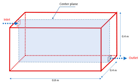
Figure 1.
Geometric parameters of the first physical experiment.
The spatial variation of the air velocity and the particle concentration profiles (within the center plane) were measured using a phase Doppler anemometer.
- (b)
- Second validation experiment
The second experiment focused on studying the spatial deposition of aerosolized Staphylococcus aureus in an aerobiology empty room. The room dimensions were 4.26 m × 3.36 m × 2.26 m with insulated walls, and the room was supplied by a HEPA filtered air through a high-level wall-mounted diffuser. The room geometry and the locations of the velocity measuring poles are shown in Figure 2a. 2.5 μm bioaerosol particles from a pre-autoclaved six-jet collision nebulizer were injected at the room’s geometric center, and the deposition was measured using groups of five 90 mm Petri dishes (settle plates) located around specified locations on the floor surface in the room, Figure 2b. The fractional bacteria count Ci representing the normalized deposition distributions at each collection point was used to compare the experimental measurements and the CFD results.
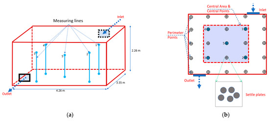
Figure 2.
Locations of velocity measuring poles and settle plates (second validation experiment). (a) Locations of velocity measuring poles. (b) Locations of settle plates on the floor (plan view).
3.4.2. Results of Model Validation
- (a)
- First validation experiment
Figure 3a shows the x-direction air velocity profiles at the chamber’s central location (X = 0.4 m). The velocity profile produced by the numerical model from the current study is compared to the numerical model developed by Alvin, 2011 [37] and the experimental data (measured by Chen, 2006) [35]. The experimental data are well predicted by the model developed in this study.
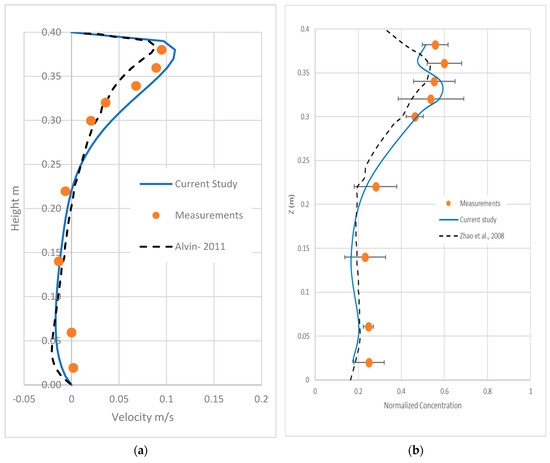
Figure 3.
Measured and calculated velocity and concentration profiles for the first validation experiment at the center plane at x = 0.4 m. (a) Velocity profile. (b) Particle concentration profile.
Figure 3b shows the simulated particle concentration’s comparisons by the current CFD model, the CFD model by Zhao et al. [38], and the experimental data [35]. The developed model (in this study) reasonably agrees well with the experimental data. In the original data measurements [35], the range of error is only given for the concentration measurements, and the accuracy of the velocity measurements is not mentioned. However, it is expected that the range of errors in measuring the point air velocity are quite small compared to the corresponding errors in the concentration measurements.
- (b)
- Second validation experiment
Figure 4a shows the air velocity magnitudes’ longitudinal profiles at pole number 2 in the room. The figure presents the experimental measurements from anemometry readings and compares the CFD results of models developed by the authors and other researchers in previous studies. The velocity measurements at the other poles are disregarded as they were significantly influenced by high noise to the extent that their reedings fall below the Testo’s measuring capability [46].
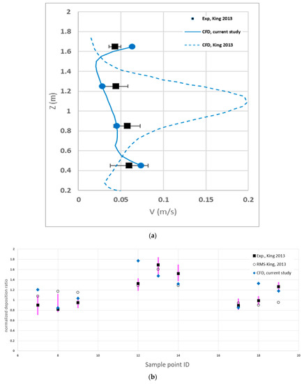
Figure 4.
Comparison of the experimental and calculated values for the second validation experiment. (a) Velocity profile at pole 2. (b) Normalized deposition ratio at the room central locations shown in Figure 2b.
The recent CFD model by the authors generally gives a better match to the measurements, especially at pole 2; however, discrepancies between the developed CFD model and measurements are noticed at poles 1 and 4. Similar differences were also found in the previous CFD model developed by King et al., 2013. It is also found that the current CFD model gives velocity predictions slightly better than the previous CFD RMS model provided by King, 2013 [27].
Figure 4b presents the normalized experimental deposition ratio and numerical predictions from the CFD models at the empty room’s central nine points. Comparison with the simulation results shows some discrepancies between the CFD model results and the measurements; however, the CFD model generally predicted the spatial variations in the normalized deposition values reasonably well.
3.5. Classroom Case Description
3.5.1. Classroom Layout and Facilities
The case study in-hand is for a typical medium-size classroom that can comfortably hold 25 students. The room dimensions were 735 cm in length by 670 cm in width, and 275 cm in height, Figure 5a. The room had double-leaf French doors of width equal to 77 cm per leaf and a height of 207 cm. The height of the underneath door slot varied from 6 to 9 mm. There was an emergency exit door located on the front wall of the entrance door. However, the emergency exit door is kept closed during regular use, and therefore this is not considered in the analysis.
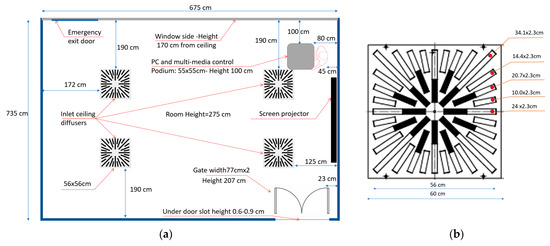
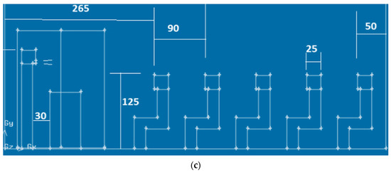
Figure 5.
Main geometric dimensions of the exam room. (a) The layout of a typical classroom. (b) Main dimensions of the inlet ceiling swirl diffuser. (c) Locations of students’ seats.
The classroom furniture includes a multi-media control podium of dimensions 55 cm by 55 cm and the podium height of 100 cm from the room floor. It also contains 25 chairs (one chair for each student). Chairs are distributed in five rows, and each row includes five seats. The distance between each row is 90 cm, and the average height of students’ faces while being seated is 125 cm, whereas the height of the instructor’s face while standing is 175 cm.
In order to model the instructor and the students in class, a simplified geometry of the typical manikin (that represents the body of the instructor or the students) was adopted as shown in Figure 5c. The use of simplified shape of human body reduces the simulation time strongly. This simplification was applied by several researchers with the aim of reducing the number of nodes and simulation time [17,18,32,35]. Taghinia et al. [47] found that simulating a real manikin improved the velocity profile only by 3–10% compared to cubic manikin. Bonello et al. [48] and Cook et al. [49] concluded that real, complex modelling of the human body has negligible impact on the surrounding climate compared to simplified cuboids.
3.5.2. Ventilating System
Four ceiling inlet diffusers centrally ventilate the classroom. Each inlet panel is 56 cm square in shape, and it includes a swirl diffuser with manually adjustable vanes. Figure 5b shows the typical geometric details of the openings in the inlet ceiling diffuser found in the classroom.
To measure the inlet airflow that exits from the swirl diffuser, a cardboard skirt of dimensions 60 cm by 60 cm with an eccentric square notch of dimensions 10 cm × 10 cm was built and used with a hot wire anemometer (model: testo 435-4, resolution: 0.01 m/s and range: 0 to 20 m/s). The measured airflow from the ceiling swirl diffuser ranged from 45 to 50 l/s, and the total inlet airflow from the four diffusers was about 180 to 200 l/s, which is equivalent to an air change rate of about 5 ACH.
3.5.3. Development of Scenarios
Five scenarios were developed (R1 to R5) to study the effects of the ventilation rate and entrance door opening on the students’ exposure to hazards. Moreover, two additional runs (R6 and R7) were conducted to study the effect of using different particle sizes. Table 2 lists the scenarios that we numerically analyzed. Four ventilation rates were examined. The 100% ventilation case (R3) reflects the classroom’s current ventilation rate, of 200 l/s.
Table 2.
Characteristics of the conducted numerical runs.
According to ASHRAE standards [44], the minimum ventilation rate for a typical lecture room is 3.8 l/s/person, which results in a total ventilation supply of 98 l/s for 25 students in addition to the instructor. This minimum ventilation rate is reflected by scenario R2, and it will be considered the reference case for comparison with other scenarios. Scenario R1 assumes no-ventilation is included in the list to discuss when no ventilation is provided due to sudden power failure during an emergency situation.
3.5.4. Development of CFD Model for Lecture Room
- (a)
- Model Description
In this study, the commercial package FLUENT-ANSYS was used to simulate the airflow and airborne aerosols for the lecture room shown in Figure 5. In this regard, a 3-D unsteady state airflow model was developed.
All the conducted scenarios assume isothermal conditions with a constant air temperature of the order of 20 °C. The effect of thermal variation was neglected, to reduce the computational time and focus on the other parameters to be investigated, such as the ventilation rate.
We assumed that the students entered the exam room to take a short-written exam or quiz in all simulations. An instructor who is unaware of being infected is supposed to give the students short verbal instructions related to the exam during the first 3 min while disclosing his/her face mask. We assumed that the oral instructions result in a spread of unified/single aerosol size droplets of 5, 2.5 or 1 μm that will initially spread out with an initial air velocity of 4.4 m/s and were ejected from the mouth of the infected instructor. For model simplicity, the instructor’s mouth was idealized to be rectangular in shape with 2 cm in width and 0.5 cm in height. Some assumptions were previously adopted by other researchers [27,50].
- (b)
- Model Discretization and CGI Analysis
Figure 6 shows the mesh discretization of the swirl ceiling diffuser. The first layer of grid points on all the students is carefully taken in the near-wall mesh zone to keep the y+ value within an acceptable limit (maximum below 10).
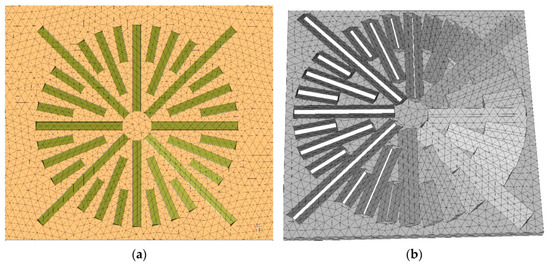
Figure 6.
Mesh discretization of the swirl ceiling diffuser. (a) 2D view. (b) 3D view.
For the whole class, a mesh of 1,600,000 cells was constructed.
Numerical models generally use discrete methods to convert the governing partial differential equations into algebraic equations. All discrete methods introduce discretization errors that might be significant enough to ruin the accuracy of the produced numerical solutions. Therefore, the computational fluid dynamics community and many other CFD-reputable journals require discretization error estimation as prerequisites for publishing any CFD paper.
The grid convergence index (GCI) is a new discretization error estimation technique. The GCI is calculated to answer whether the adopted mesh in the simulation is refined enough or not [51]. A minimum of two mesh solutions is required, but three is recommended to calculate the GCI.
In the current study, four sizes of meshes depending on the side length of the cells on the students’ faces and bodies were tested to calculate the GCI, which were: 10, 8, 6, and 5 cm, where the accuracy of the output results “the sum of the DPM concentrations on the bodies and the faces of all the students at 90 and 150 s” is checked. GCI was calculated using the method described in research [51] for the case of no ventilation. GCI fine was less than 1% for mesh 5 cm and less than 1.8% for the mesh of 6 cm. The approximate error was less than 2% for the mesh 5 cm and less than 3.5% for the mesh 6 cm. In this regard, the mesh 5 cm of tetrahedral cells was selected for all further analyses.
4. Results and Discussion
4.1. Induced Air Field by Swirl Ceiling Diffuser
Figure 7 shows the airflow pathlines from the ceiling diffuser for the 50% ventilation rate case. The figure shows only those pathlines emerging from the ceiling diffuser located just above the instructor. The pathlines from the other three diffusers were hidden, seeking figure clarity.
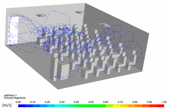
Figure 7.
Pathlines emerging from the ceiling diffuser above the instructor (Run R2-Time 180 s).
The figure shows the complicated airflow pattern that results from the swirl ceiling diffusers. It also shows that the typical average air velocity was less than 0.2 m/s.
4.2. Aerosol Droplets Tracking
Figure 8 shows the aerosol droplet time tracking with the time course for the different ventilation rates.
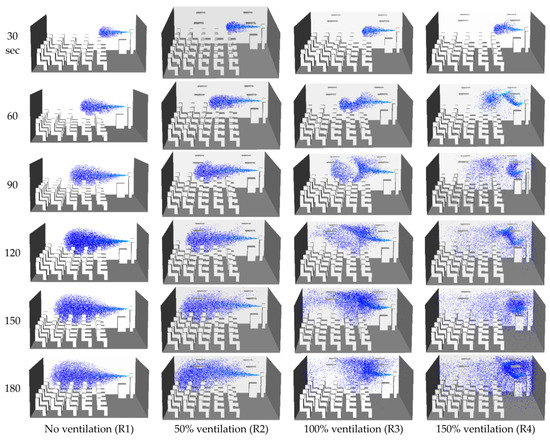
Figure 8.
Time tracking of aerosol droplets with the time course and different ventilation rates (scenarios R1–R4).
Figure 9 presents the time residence of the dispersed aerosol droplets after 180 s from the instructor’s start for the different ventilation scenarios. It is noted that the velocity field for scenarios R3 and R4 is remarkably different from scenarios R1 and R2.
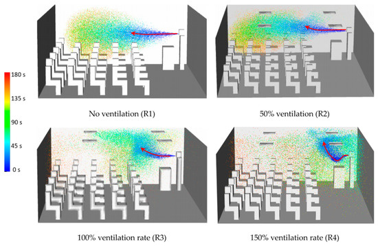
Figure 9.
Time residence for dispersed aerosol droplets after 180 s.
As the ventilation rate increases, the aerosol droplets’ upward entrainment (induction) due to the generated swirl air flow by the swirl diffuser becomes more apparent and more robust. The entrainment process that is caused by the swirl diffuser was previously discussed by other researchers [17]. This entrainment process will help in reducing the risk of student exposure to harmful aerosol droplets.
Figure 10 shows an example of the students’ exposed areas to the traces of aerosol droplets colored by the normalized concentration under no ventilation conditions. Some students were exposed to aerosol droplets, whereas others were not. Exposed students differed in the body’s exposed location and whether it was the face, the body, or both, as shown in Figure 10.
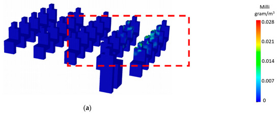
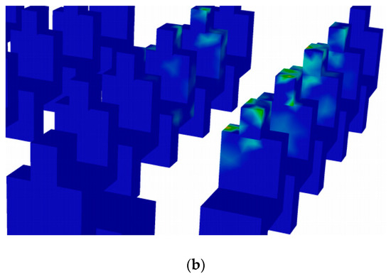
Figure 10.
Students exposure areas after 180 s (no ventilation case-R1). (a) Full class. (b) Zoom-in of the dashed window shown in Figure 10a.
4.3. Discussion
Figure 11a shows a double y plot for NAC and SNAC with the (VRR) in the x-axis. The figure shows the normalized average concentration (NAC) of aerosol droplets received by students’ faces only and body only for the different ventilation rate cases.
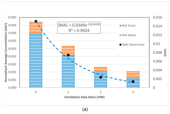
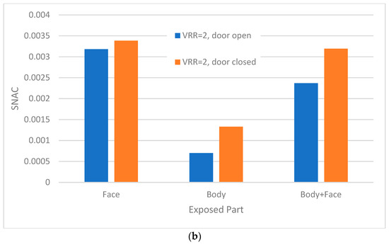
Figure 11.
Variation of (NAC) and (SNAC) with the ventilation rate and gate status. (a) Variation of (NAC) and (SNAC) with the ventilation rate. (b) Variation of the total (SNAC) (body+face) with door status (open/closed).
It is clear that, as ventilation increased, the average NAC received by students generally decreased. On the other hand, as the ventilation rate increased, the number of students exposed to the aerosol droplets increased as well. This finding is based on the model results; however, it is not depicted in Figure 11.
The SNAC was calculated and is also presented in Figure 11a. We found that, as the ventilation rate increased, SNAC decreased exponentially, and it tended to asymptotically reach zero SNAC at the theoretically infinite value of the ventilation rate. The results indicate that increasing the ventilation rate ratio (VRR > 3) is expected to have a marginal effect on reducing the SNAC.
Figure 11b presents a comparison between the open and the closed-door cases, assuming a ventilation rate double the minimum value (VRR = 2). The figure shows how SNAC varies for the different exposed parts of the body. It can be concluded that opening the classroom door helped reduce the SNAC and also reduce the risk of exposure to harmful aerosols by about 26 percent.
Figure 12 shows a double y-plot for the variations of NAC and SNAC with the particle/droplet size in the x-axis. Both NAC and SNAC decreased as droplet size increased, and SNAC’s trendline appears to be quadratic with the droplet size. Based on the SNAC values for the whole body, the 5 μm size droplets appear to be less hazardous as they resulted in an 87% reduction in exposure when compared with the small 1 μm size droplets.
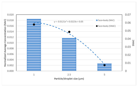
Figure 12.
Variation of (NAC) and (SNAC) with particle/droplet size.
Figure 13 shows how the exceedance in exposure ratio (EER) index varied with the different ventilation rates after 180 s. The figure indicates that the highest exposure to droplets location was not in the front row but in the third row (for the scenario cases: R1 and R2). It can also be noted that the maximum scored values of EER were 3.5 and 2.15 for the no-ventilation (Figure 13a) and 50% ventilation (Figure 13b) cases, respectively. This means that, for the case of VRR = 0 (Figure 13a), the worst-case student had a risk of exposure to droplets that exceeded the reference average by 3.5 times, whereas the worst-case student for the case of VRR = 1 (Figure 13b) (run R2), had a corresponding risk that exceeded the reference average by 2.15 times. When the ventilation rate reached VRR ≥ 2 (Figure 13c,d), the location points of high exposure were not distinguishable, and almost all students had a negative EER, which means the majority were exposed to risk less than the reference average.
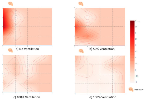
Figure 13.
The exceedance in exposure ratio (EER) after 180 s.
5. Conclusions
Our study numerically simulated the transmission of exhaled droplets in a typical 25-seat exam room. The study numerically tracked the ejected droplets from the instructor’s mouth while giving 3-min exam guidelines. The model was built using ANSYS-Fluent-Workbench where the RNG k-epsilon turbulence model and the DPM module were chosen for the droplet transmission simulation. The exhaled droplets (of 5, 2.5, or 1 µm in size) were initially spread out from the instructor’s mouth with an initial air velocity of 4.4 m/s.
Two key parameters were considered for investigations to study their effects on the students’ exposure to the harm droplets: the ventilation rate and the room’s door status. Two dimensionless indices were introduced to facilitate the study assessment. The first was a number called the specific normalized average concentration (SNAC), which gives a lump-sum estimate for the average students’ exposure for the exam room. The second dimensionless number was the exceedance in exposure ratio (EER), which provides insight into the spatial variability of the students’ exposure to help identify the locations of high-risk spots within the room. The main findings of the study are as follows:
- The contour mapping of the EER within the exam room, after 180 s, revealed that the students sitting in front of the instructor, especially in the second and third rows, were more susceptible to infection if the ventilation rate does not exceed the minimum recommended ventilation rate by ASHRAE. On the other hand, and as expected, students sitting beside the wall far from the instructor were not affected.
- The dispersion of the exhaled droplets inside the room was improved significantly by increasing the ventilation rate.
- Increasing the ventilation rate increased the number of affected students. However, it decreased the concentrations to which they were significantly exposed.
- Increasing the ventilation rate decreased the specific normalized average concentration (SNAC) exponentially. Nevertheless, increasing the ventilation rate ratios above three is expected to have a non-tangible effect on reducing the harmful droplets’ exposure. However, more analysis may be required in this regard.
- Keeping the room’s main door open at a ventilation rate ratio of 2 reduced the risk of exposure (to the harmful aerosol droplets) by 26%.
- Based on the SNAC values for the whole body, the large size (5 μm) droplets appeared to be less hazardous as they resulted in an 87% reduction in exposure when compared with the small 1 μm size droplets.
- Some students might be subjected to a high risk of exposure (to harmful droplets) that exceeded 3.5 times the average reference risk in the case of no ventilation.
In this paper, the normal speaking process of the polluting instructor was modeled. However, coughing or sneezing processes with high initial velocities may result in different transmission behavior of exhaled droplets. Having a student as a polluting source may need to be further studied when sitting at various locations. These points and other scenarios are essential to further investigate to enhance our understanding of droplet transmission in education facilities.
Author Contributions
Conceptualization, M.I.F. and A.F.N.; methodology, M.H.E. and M.I.F.; software, M.H.E. and M.I.F.; validation, M.I.F., A.F.N. and M.H.E.; formal analysis, M.H.E. and A.F.N.; investigation, A.F.N. and M.H.E.; resources, A.F.N.; data curation, M.H.E.; writing—original draft preparation, M.H.E. and A.F.N.; writing—review and editing, M.H.E., M.I.F. and A.F.N.; visualization, M.H.E. and A.F.N.; supervision, M.I.F.; project administration, M.I.F.; funding acquisition, N/A. All authors have read and agreed to the published version of the manuscript.
Funding
This research received no external funding.
Institutional Review Board Statement
Not applicable.
Informed Consent Statement
Not applicable.
Data Availability Statement
Data are available on request from the authors.
Acknowledgments
The authors would like to thank Ahmed Ismail Farouk for his assistance in developing the second validation model’s geometry.
Conflicts of Interest
The authors declare no conflict of interest.
References
- WHO. Summary of Probable SARS Cases with Onset of Illness from 1 November 2002 to 31 July 2003. Available online: https://www.who.int/csr/sars/country/table2004_04_21/en/ (accessed on 15 August 2020).
- Dawood, F.S.; Iuliano, A.D.; Reed, C.; Meltzer, I.M.; Shay, D.; Cheng, P.-Y.; Bandaranayake, D.; Breiman, R.F.; Brooks, W.A.; Buchy, P.; et al. Estimated Global Mortality Associated with the First 12 Months of 2009 Pandemic Influenza a H1N1 Virus Circulation: A Modelling Study. Lancet Infect. Dis. 2012, 12, 687–695. [Google Scholar] [CrossRef]
- Peck, K.; Burch, C.; Heise, M.T.; Baric, R.S. Coronavirus Host Range Expansion and Middle East Respiratory Syndrome Coronavirus Emergence: Biochemical Mechanisms and Evolutionary Perspectives. Annu. Rev. Virol. 2015, 2, 95–117. [Google Scholar] [CrossRef] [PubMed]
- World Health Organization. WHO Coronavirus (COVID-19) Dashboard. Available online: https://covid19.who.int/ (accessed on 21 September 2021).
- Asadi, S.; Bouvier, N.; Wexler, A.S.; Ristenpart, W.D. The Coronavirus Pandemic and Aerosols: Does COVID-19 Transmit via Expiratory Particles? Aerosol Sci. Technol. 2020, 54, 635–638. [Google Scholar] [CrossRef] [PubMed]
- Burke, R.M.; Midgley, C.M.; Dratch, A.; Fenstersheib, M.; Haupt, T.; Holshue, M.; Ghinai, I.; Jarashow, C.; Lo, J.; McPherson, D.T.; et al. Active Monitoring of Persons Exposed to Patients with Confirmed COVID-19—United States, January–February 2020. MMWR Morb. Mortal. Wkly. Rep. 2020, 69, 245–246. [Google Scholar] [CrossRef]
- Chan, J.F.-W.; Yuan, S.; Kok, K.-H.; To, K.K.-W.; Chu, H.; Yang, J.; Xing, F.; Liu, J.; Yip, C.C.-Y.; Poon, R.W.-S.; et al. A Familial Cluster of Pneumonia Associated with the 2019 Novel Coronavirus Indicating Person-To-Person Transmission: A Study of a Family Cluster. Lancet 2020, 395, 514–523. [Google Scholar] [CrossRef]
- Hadei, M.; Hopke, P.K.; Jonidi, A.; Shahsavani, A. A Letter about the Airborne Transmission of SARS-CoV-2 Based on the Current Evidence. Aerosol Air Qual. Res. 2020, 20, 911–914. [Google Scholar] [CrossRef]
- Huang, C.; Wang, Y.; Li, X.; Ren, L.; Zhao, J.; Hu, Y.; Zhang, L.; Fan, G.; Xu, J.; Gu, X.; et al. Clinical Features of Patients Infected with 2019 Novel Coronavirus in Wuhan, China. Lancet 2020, 395, 497–506. [Google Scholar] [CrossRef]
- Jones, R.M.; Brosseau, L.M. Aerosol Transmission of Infectious Disease. J. Occup. Environ. Med. 2015, 57, 501–508. [Google Scholar] [CrossRef]
- Li, Q.; Guan, X.; Wu, P.; Wang, X.; Zhou, L.; Tong, Y.; Ren, R.; Leung, K.; Lau, E.; Wong, J.Y.; et al. Early Transmission Dynamics in Wuhan, China, of Novel Coronavirus–Infected Pneumonia. N. Engl. J. Med. 2020, 382, 1199–1207. [Google Scholar] [CrossRef] [PubMed]
- Liu, Y.; Ning, Z.; Chen, Y.; Guo, M.; Liu, Y.; Gali, N.K.; Sun, L.; Duan, Y.; Cai, J.; Westerdahl, D.; et al. Aerodynamic Analysis of SARS-CoV-2 in Two Wuhan Hospitals. Nature 2020, 582, 557–560. [Google Scholar] [CrossRef] [PubMed]
- Morawska, L.; Cao, J. Airborne Transmission of SARS-CoV-2: The World Should Face the Reality. Environ. Int. 2020, 139, 105730. [Google Scholar] [CrossRef]
- Mittal, R.; Ni, R.; Seo, J.-H. The Flow Physics of COVID-19. J. Fluid Mech. 2020, 894. [Google Scholar] [CrossRef]
- Van Doremalen, N.; Bushmaker, T.; Morris, D.H.; Holbrook, M.G.; Gamble, A.; Williamson, B.N.; Tamin, A.; Harcourt, J.L.; Thornburg, N.J.; Gerber, S.I.; et al. Aerosol and Surface Stability of SARS-CoV-2 as Compared with SARS-CoV-1. N. Engl. J. Med. 2020, 382, 1564–1567. [Google Scholar] [CrossRef] [PubMed]
- Bourouiba, L.; Dehandschoewercker, E.; Bush, J.W.M. Violent Expiratory Events: On Coughing and Sneezing. J. Fluid Mech. 2014, 745, 537–563. [Google Scholar] [CrossRef]
- He, Q.; Niu, J.; Gao, N.; Zhu, T.; Wu, J. CFD Study of Exhaled Droplet Transmission between Occupants under Different Ventilation Strategies in a Typical Office Room. Build. Environ. 2011, 46, 397–408. [Google Scholar] [CrossRef] [PubMed]
- Richmond-Bryant, J. Transport of Exhaled Particulate Matter in Airborne Infection Isolation Rooms. Build. Environ. 2009, 44, 44–55. [Google Scholar] [CrossRef]
- Wei, J.; Li, Y. Enhanced Spread of Expiratory Droplets by Turbulence in a Cough Jet. Build. Environ. 2015, 93, 86–96. [Google Scholar] [CrossRef]
- Xie, X.; Li, Y.; Chwang, A.T.Y.; Ho, P.L.; Seto, W.H. How Far Droplets Can Move in Indoor Environments? Revisiting The Wells Evaporation? Falling Curve. Indoor Air 2007, 17, 211–225. [Google Scholar] [CrossRef]
- Morawska, L.; Johnson, G.; Ristovski, Z.; Hargreaves, M.; Mengersen, K.; Corbett, S.; Chao, Y.H.C.; Li, Y.; Katoshevski, D. Size Distribution and Sites of Origin of Droplets Expelled from the Human Respiratory Tract during Expiratory Activities. J. Aerosol Sci. 2009, 40, 256–269. [Google Scholar] [CrossRef]
- Chao, C.; Wan, M.P.; Morawska, L.; Johnson, G.; Ristovski, Z.; Hargreaves, M.; Mengersen, K.; Corbett, S.; Li, Y.; Xie, X.; et al. Characterization of Expiration Air Jets and Droplet Size Distributions Immediately at the Mouth Opening. J. Aerosol Sci. 2009, 40, 122–133. [Google Scholar] [CrossRef]
- Kwon, S.-B.; Park, J.; Jang, J.; Cho, Y.; Park, D.-S.; Kim, C.; Bae, G.-N.; Jang, A. Study on the Initial Velocity Distribution of Exhaled Air from Coughing and Speaking. Chemosphere 2012, 87, 1260–1264. [Google Scholar] [CrossRef] [PubMed]
- Zhang, H.; Li, D.; Xie, L.; Xiao, Y. Documentary Research of Human Respiratory Droplet Characteristics. Procedia Eng. 2015, 121, 1365–1374. [Google Scholar] [CrossRef]
- Liu, Y.; Ning, Z.; Chen, Y.; Guo, M.; Liu, Y.; Gali, N.K.; Sun, L.; Duan, Y.; Cai, J.; Westerdahl, D. Aerodynamic Characteristics and RNA Concentration of SARS-CoV-2 Aerosol in Wuhan Hospitals during COVID-19 Outbreak. BioRxiv 2020, 982637. [Google Scholar] [CrossRef]
- Noakes, C.J.; Sleigh, P.A.; Escombe, A.R.; Beggs, C.B.; Sleigh, A. Use of CFD Analysis in Modifying a TB Ward in Lima, Peru. Indoor Built Environ. 2006, 15, 41–47. [Google Scholar] [CrossRef]
- King, M.-F.; Noakes, C.; Sleigh, P.; Camargo-Valero, M. Bioaerosol Deposition in Single and Two-Bed Hospital Rooms: A Numerical and Experimental Study. Build. Environ. 2013, 59, 436–447. [Google Scholar] [CrossRef]
- King, M.-F.; Noakes, C.J.; Sleigh, P.A. Modeling Environmental Contamination in Hospital Single- And Four-Bed Rooms. Indoor Air 2015, 25, 694–707. [Google Scholar] [CrossRef]
- Loomans, M.; de Visser, I.; Loogman, J.; Kort, H. Alternative Ventilation System for Operating Theaters: Parameter Study and Full-Scale Assessment of the Performance of a Local Ventilation System. Build. Environ. 2016, 102, 26–38. [Google Scholar] [CrossRef][Green Version]
- Verma, T.N.; Sahu, A.K.; Sinha, S.L. Study of Particle Dispersion on One Bed Hospital using Computational Fluid Dynamics. Mater. Today Proc. 2017, 4, 10074–10079. [Google Scholar] [CrossRef] [PubMed]
- Zhao, B.; Li, X.; Zhang, Z.; Huang, D. Comparison of Diffusion Characteristics of Aerosol Particles in Different Ventilated Rooms by Numerical Method. ASHRAE Trans. 2004, 110, 88–96. [Google Scholar]
- Zhao, B.; Zhang, Y. Analysis of Particle Pollution in an Office by the Concept of Perceived Particle Intensity. Indoor Built Environ. 2006, 15, 463–472. [Google Scholar] [CrossRef]
- La, A.; Zhang, Q. Experimental Validation of CFD Simulations of Bioaerosol Movement in a Mechanically Ventilated Airspace. Can. Biosyst. Eng. 2019, 5.01–5.14. [Google Scholar] [CrossRef]
- Zhang, Y.; Feng, G.; Kang, Z.; Bi, Y.; Cai, Y. Numerical Simulation of Coughed Droplets in Conference Room. Procedia Eng. 2017, 205, 302–308. [Google Scholar] [CrossRef]
- Chen, F.; Yu, S.; Lai, A.C. Modeling Particle Distribution and Deposition in Indoor Environments with a New Drift–Flux Model. Atmos. Environ. 2006, 40, 357–367. [Google Scholar] [CrossRef]
- Chen, Q. Comparison of Differentk-Ε Models for Indoor Air Flow Computations. Numer. Heat Transfer Part B Fundam. 1995, 28, 353–369. [Google Scholar] [CrossRef]
- Lai, A.C.K.; Chen, F. Corrigendum to: “Modeling of Particle Deposition and Distribution in a Chamber with a Two-Equation Reynolds-Averaged Navier–Stokes model”. J. Aerosol Sci. 2011, 42, 497–498. [Google Scholar] [CrossRef]
- Zhao, B.; Yang, C.; Yang, X.; Liu, S. Particle Dispersion and Deposition in Ventilated Rooms: Testing and Evaluation of Different Eulerian and Lagrangian Models. Build. Environ. 2008, 43, 388–397. [Google Scholar] [CrossRef]
- Zoka, H.M.; Moshfeghi, M.; Bordbar, H.; Mirzaei, P.; Sheikhnejad, Y. A CFD Approach for Risk Assessment Based on Airborne Pathogen Transmission. Atmosphere 2021, 12, 986. [Google Scholar] [CrossRef]
- Shao, S.; Zhou, D.; He, R.; Li, J.; Zou, S.; Mallery, K.; Kumar, S.; Yang, S.; Hong, J. Risk Assessment of Airborne Transmission of COVID-19 by Asymptomatic Individuals under Different Practical Settings. J. Aerosol Sci. 2021, 151, 105661. [Google Scholar] [CrossRef]
- Salmela, A.; Kokkonen, E.; Kulmala, I.; Veijalainen, A.-M.; Van Houdt, R.; Leys, N.; Berthier, A.; Viacheslav, I.; Kharin, S.; Morozova, J.; et al. Production and Characterization of Bioaerosols for Model Validation in Spacecraft Environment. J. Environ. Sci. 2018, 69, 227–238. [Google Scholar] [CrossRef]
- Hu, S. Airflow Characteristics in the Outlet Region of a Vortex Room Air Diffuser. Build. Environ. 2003, 38, 553–561. [Google Scholar] [CrossRef]
- Liu, Z.; Wang, L.; Rong, R.; Fu, S.; Cao, G.; Hao, C. Full-Scale Experimental and Numerical Study of Bioaerosol Characteristics Against Cross-Infection in a Two-Bed Hospital Ward. Build. Environ. 2020, 186, 107373. [Google Scholar] [CrossRef]
- ASHRAE Addendum. Ventilation for Acceptable Indoor Air Quality, ANSI/ASHRAE Addendum p to ANSI/ASHRAE Standard 62.1-2013; ASHRAE: Atlanta, GA, USA, 2015. [Google Scholar]
- ANSYS. Fluent Theory Guide Release 15.0; ANSYS, Inc.: Canonsburg, PA, USA, 2013; pp. 1–814. [Google Scholar]
- King, M.-F.; (Research Fellow, School of Civil Engineering, University of Leeds, Leeds, UK). Personal communication, 1 June 2020.
- Taghinia, J.H.; Rahman, M.; Lu, X. Effects of Different CFD Modeling Apsproaches and Simplification of Shape on Prediction of Flow Field Around Manikin. Energy Build. 2018, 170, 47–60. [Google Scholar] [CrossRef]
- Bonello, M.; Micallef, D.; Borg, S.P. Humidity Distribution in High-Occupancy Indoor Micro-Climates. Energies 2021, 14, 681. [Google Scholar] [CrossRef]
- Cook, M.; Cropper, P.; Fiala, D.; Yousaf, R.; Bolineni, S.; van Treeck, C. Coupled CFD and Thermal Comfort Modeling in Cross-Ventilated Classrooms. ASHRAE Trans. 2013, 119, 1–8. [Google Scholar]
- Zhiqiang, K.; Yixian, Z.; Hongbo, F.; Guohui, F. Numerical Simulation of Coughed Droplets in the Air-Conditioning Room. Procedia Eng. 2015, 121, 114–121. [Google Scholar]
- Journal of Fluids Engineering Editorial Policy, Statement on the Control of Numerical Accuracy. Available online: https://www.asme.org/wwwasmeorg/media/resourcefiles/shop/journals/jfenumaccuracy.pdf (accessed on 16 September 2021).


Publisher’s Note: MDPI stays neutral with regard to jurisdictional claims in published maps and institutional affiliations. |
© 2021 by the authors. Licensee MDPI, Basel, Switzerland. This article is an open access article distributed under the terms and conditions of the Creative Commons Attribution (CC BY) license (https://creativecommons.org/licenses/by/4.0/).