Article

Biosignal-Based Driving Skill Classification Using Machine Learning: A Case Study of Maritime Navigation

1
Department of Technology and Safety, UiT The Arctic University of Norway, 9019 Tromsø, Norway
2
Department of Automation and Processing Technology, UiT The Arctic University of Norway, 9019 Tromsø, Norway
3
Department of Computer Science, UiT The Arctic University of Norway, 9019 Tromsø, Norway
*
Author to whom correspondence should be addressed.
Appl. Sci. 2021, 11(20), 9765; https://doi.org/10.3390/app11209765
Submission received: 26 September 2021 / Revised: 5 October 2021 / Accepted: 15 October 2021 / Published: 19 October 2021
(This article belongs to the Topic Artificial Intelligence in Sensors)

Abstract

:
This work presents a novel approach to detecting stress differences between experts and novices in Situation Awareness (SA) tasks during maritime navigation using one type of wearable sensor, Empatica E4 Wristband. We propose that for a given workload state, the values of biosignal data collected from wearable sensor vary in experts and novices. We describe methods to conduct a designed SA task experiment, and collected the biosignal data on subjects sailing on a 240° view simulator. The biosignal data were analysed by using a machine learning algorithm, a Convolutional Neural Network. The proposed algorithm showed that the biosingal data associated with the experts can be categorized as different from that of the novices, which is in line with the results of NASA Task Load Index (NASA-TLX) rating scores. This study can contribute to the development of a self-training system in maritime navigation in further studies.

1. Introduction

The classic methodology for maritime training generally involves multiple sensors in addition to simulator for improving situation awareness (SA) in maritime navigation and seafaring skills [1]. The purpose of this study is to determine if a wearable sensor can be used to detect stress changes with skills during a maritime navigation task. We define stress as the task requirement for both experienced seafarers (experts) and novices (students). We collected the biosignal data of subjects for indicating the stress differences under the SA tasks during maritime navigation. Biosignal data including electrodermal activity (EDA), body temperature, blood volume pulse (BVP) and heart rate (HR) are some of the indicators to present the stress level, since stress is the body’s reaction to pressure and a physical response to situations in which people feel threatened.
Safe maritime navigation in the Arctic region is challenging because there is less infrastructure, long distances between harbours and harsh weather conditions [2]. However, the safety of the Arctic route is of great significance to the economic development of Scandinavia, and at the same time has an impact on environmental protection and the safe growth of marine life. The sailing route in the Vessel Traffic Services area on the west coast of Norway, north of Bergen, is a typical route for training the seafarers because of its complexity and busy traffic, especially for training SA in the safety of the maritime navigation.
In maritime, the study of situation awareness (SA) has always been an important topic of discussion. Studies show that many ship collisions and groundings occur due to navigators’ erroneous SA. Grech et al. [3] found that 71% of navigators’ errors can be attributed to SA-related problems. Therefore, training maritime students to improve their SA is one of the most important tasks in maritime education.
In maritime navigation, an experienced navigator can keep track of multiple tasks and deal with more complex situations without losing SA as compared to a novice. For a novice, managing multiple tasks required for navigation can be quite challenging [4]. As navigating a ship can be stressful, managing this stress can bring different results. In this study, we aim to investigate whether there are differences in the biosignals between the experts and novices for a given sailing task.

1.1. Related Research Work

There are only a few works related to performance assessment of SA objectively during maritime training navigation. In the existing literature, survey and interview are usually the common tools for assessing SA. From its conception, SA was defined by Endsley in 1988 as “the perception of the elements in the environment within a volume of time and space, the comprehension of their meaning, the projection of their status in the near future” [5,6]. In simple terms, it can be understood as “being aware of what is happening around you and understanding what information means to you now and in the future” [6]. In maritime operations, the awareness refers to the important information for sailing and being safe on board (particular job or goals in general), and only the situations that relate to the tasks are important to SA. For example, the navigator of a ship must be aware of other ships, the weather, the water, the grounding, and so on. When sailing a ship, during the different tasks, the navigator should be able to adjust and adapt the performance based on the current situation or the change of the situation. In order to improve the training system for SA within maritime navigation, several studies of sensor fusion technology have been used on simulators in the past few years [1,7]. However, as far as we know, use of bio-sensor data with the SA training system is not common. The main contribution of this paper is to provide a possibility for doing such research.

1.2. Objective and Contributions

The main objective of this study is to investigate the differences in the stress levels of experts and novices in SA experiment during a maritime navigation task. In this study, we investigate the following research hypotheses: First, the biosensor data from experienced experts can be distinguished from the biosensor data from students. Second, the stress levels obtained from the biosensor data show a correlation to the NASA-TLX rating results. Third, compared to the novices, the experts feel less stress during a navigation task.
The main contribution can be summarised as follows:
  • Maritime transport requires safety and security. SA in maritime is the effective understanding of activity that could impact the security and safety. This study discovers that the stress level varies according to the experience of the seafarers, which matters in the performance of SA during the maritime navigation.
  • SA training is common in the aviation domain and the maritime domain. While SA training-related stress level analysis is widely studied for aviation, SA training-related stress level analysis in maritime navigation is less studied. This paper is a pilot case study towards classifying stress level among the expert and novice seafarers. We have used a ’hybrid’ convolutional neural network approach in combination with statistical, wavelet and higher-order crossing features to classify the stress level based on biosignals during the maritime navigation. We are first extracting features and then passing those features to a Convolutional Neural Network so we refer to is as a ’hybrid Convolutional Neural Network’.

2. Methodology

In order to study the SA-based stress level analysis, we used the Kongsberg K-Sim navigation platform. Both expert and novice drivers were given the same driving scenario and their biosignals were recorded using Empatica E4 band while they were driving on the simulator. In the next sub-section we elaborate on the information about participants, materials and apparatus used for this study.

2.1. Participants

The trial was performed with 10 healthy male participants. In order to compare the performance and emotion between the experts and novice in maritime navigation tasks, both experts and novices were invited to participate in the experiment. There were five navigators with extensive experience (mean age = 41.8 years, standard deviation = 14.0 years) and five second-year students from a nautical science program with little experience (mean age = 22.8 years, standard deviation = 1.2 years). The experts had an average of 9.7 years’ experience as navigators with the longest period being 18 years and the shortest being one year.

2.2. Materials and Apparatus

A maritime navigation task was designed for testing the relationship between the navigating experience and stress. The maritime navigation task was performed on a 240° view simulator. It is equipped with the K-sim Navigation software from Kongsberg Digital. The vessel-model used in the experiment is called BULKC11 (overall length of 90 m and a moulded beam of 14 m). The task consists of two part, one part is sailing, the other part is filing the The Situation Awareness Global Assessment Technique (SAGAT) queries when the simulator screen is frozen. Each participant sailed a 40-minute voyage with four stops. Each section of the sailing lasts approximately 8 to 12 min. During the sailing section, participants had to complete the SAGAT queries in around 15 min (4 stops with an average of 4 min to answer the SAGAT queries). The whole experiment takes approximately 55 min. Figure 1 shows a participant sailing on the simulator.
During the experiment, each participant wore a wearable device for collecting the biosignal data. In this study, among the diversity of wearable sensors, a medical-grade wearable device, Empatica E4 Wristband (see Figure 2), was chosen for recording the real-time physiological data to conduct in-depth analysis. EDA and PPG sensors were equipped in the E4 Wristband that can simultaneously enable the measurement of sympathetic nervous system activity and heart rate [8]. Following is the description of the sensors in the E4 Wristband:
  • PPG Sensor: Measures blood volume pulse (BVP), from which heart rate variability can be derived [8];
  • Infrared Thermopile: Reads peripheral skin temperature [8];
  • EDA Sensor (GSR Sensor): Measures the constantly fluctuating changes in certain electrical properties of the skin [8];
  • 3-axis Accelerometer: Captures motion-based activity [8].
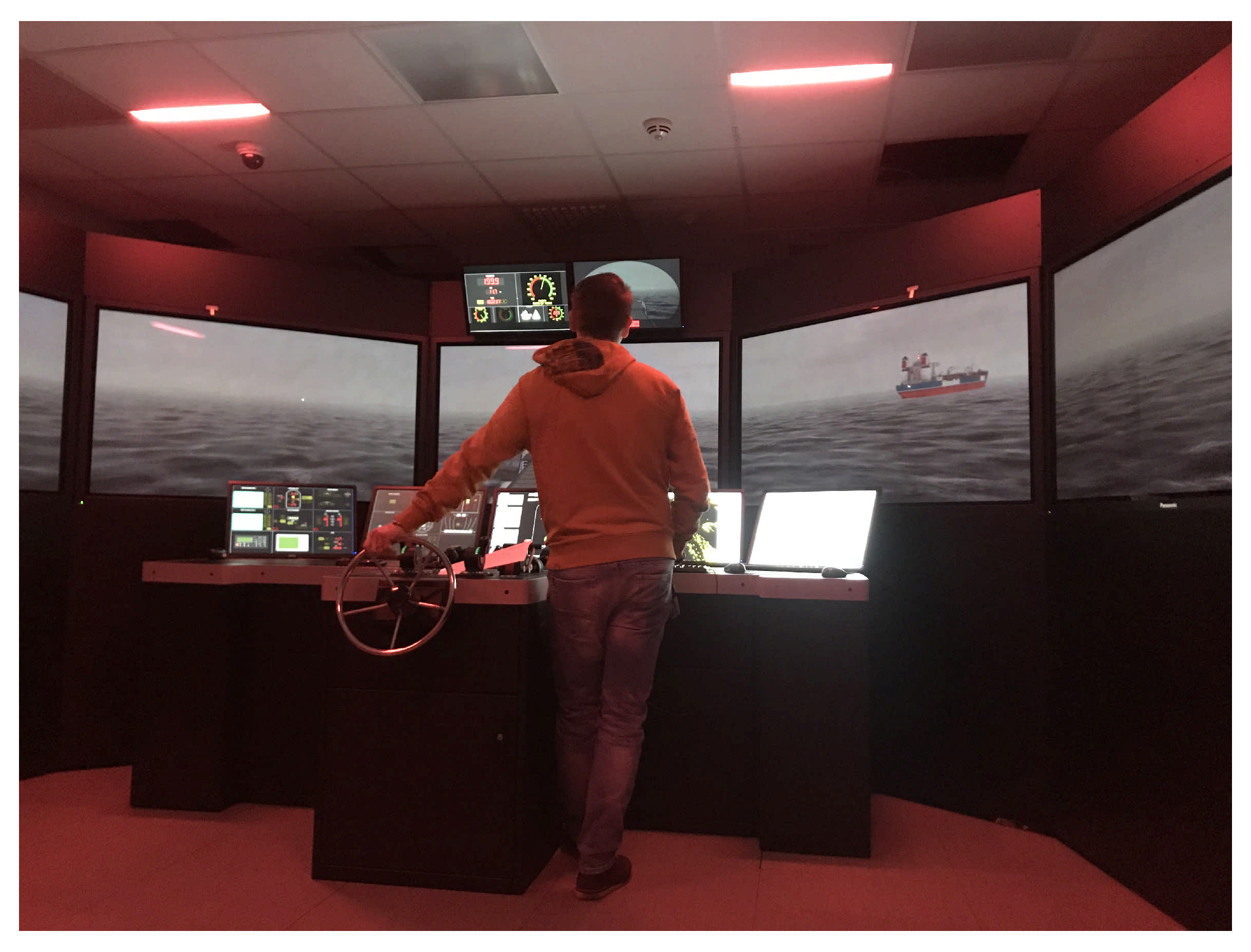
The data from E4 Wristband such as Electrodermal Activity (EDA), body temperature, blood volume pulse (BVP) and heart rate (HR) are collected and used in the analysis.

3. Experiment

In this experiment, we used NASA Task Load Index (NASA-TLX) as a reference. The rating result of NASA-TLX is a subjective measurement evaluated by the participants themselves. The result show that there are different workload and stress level between experts and students. In the light of this result, we hypothesize that it is possible to classify the biosignal data we collected during the sailing task. Hence, we extracted the features of the data and analyzed it by using convolutional neural network(CNN) in deep learning.

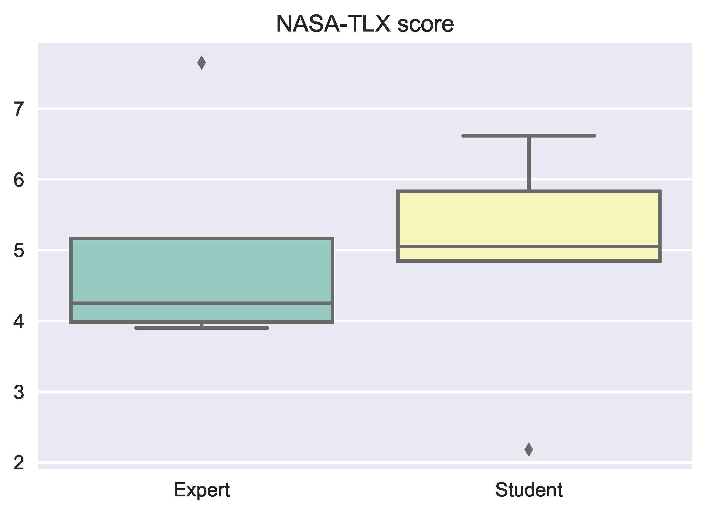
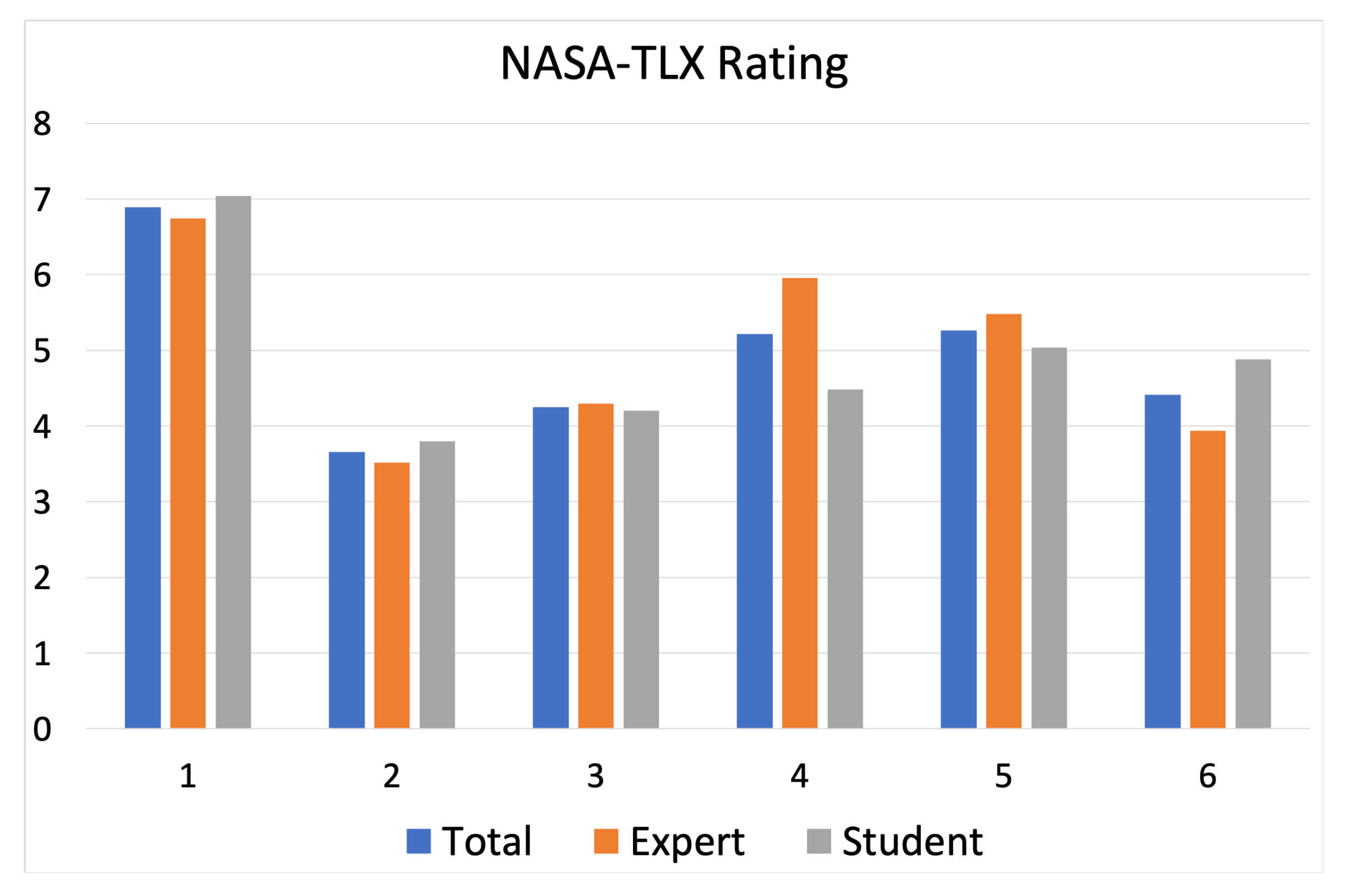
3.1. NASA Task Load Index (NASA-TLX)

The NASA Task Load Index (NASA-TLX) was used as an assessment tool to rate the perceived workload in order to assess the performance of the participants [9,10]. The six categories were required to be rated from low to high level, namely, Mental Demand, Physical Demand, Temporal Demand, Performance, Effort, and Frustration Level. The rating was transferred to a ten-point scaler scores. All the participants were given NASA-TLX after the experiment.

NASA-TLX Rating Results

There are two ways of analysing the NASA-TLX scores: one is a two-step process that needs participants to give both scores for each item and a pairwise comparison score between each pair of items (there will be in total 15 pairwise comparisons); another way is simple and convenient—calculating the average score of the six items for each participant [11,12]. In this study, only the “Raw TLX” was used [13] and the average score was calculated in order to keep the experimental validity [12]. When using the “raw TLX”, individual subscales may be dropped if less relevant to the task [14].
Figure 3 shows the average scores from the experts and students. Students considered the workload was higher than expected by experts, however, it was not highly significant. Figure 4 shows the comparison of the raw scores for students, experts and overall. The results show that both students and experts felt that the task was low in physical demand and temporal demand, while it was a highly mentally demanding. There is not much difference between the students and experts in the rating results.

3.2. Data Pre-Processing

The dataset consists of four signal channels associated with EDA, body temperature (Temp.), BVP and HR. EDA is collected from electrodermal activity sensor measured in μ S with frequency of 4 Hz. Body temperature data are measured on the Celsius (°C) scale with a frequency of 4 Hz [15]. BVP data are from photoplethysmograph (PPG) and sampled at 64 Hz [15]. HR data are the average heart rate values per second, derived directly from the BVP analysis [16]. All the signals were downsampled to 1 Hz for data analyses. The data are associated with ten participants, each participant has four sailing sections, the data can be split into forty samples (see Table 1). In order to compare the data with different resolutions, and to make it easier to analyse, we have normalized the downsampled data.
Normalization of the data is done by calculating the standard normal distribution. The standard normal distribution is the simplest case of the normal distribution when the data are standardized to have a mean of zero and a standard deviation of one [17]. Before calculating the standard normal distribution, the standardized value of the signal data is computed from the mean and standard deviation using the following formula (see Equation (1)) [18]:
z i = x i x ¯ S , i = 1 , 2 , , n
where z i = z 1 , z 2 , , z n is standardization value of the sample, x i = x 1 , x 2 , , x n is the value of the downsampled signals, x ¯ is the mean of x i on each file, S is the sample standard deviation, n is the number of the data on each file.
Finally, the standard normal distribution of the data was calculated using Equation (2) [19]:
f ( z i ) = 1 2 π e z i 2 2 , i = 1 , 2 , , n
where z i = z 1 , z 2 , , z n is standardization value of the sample and n is the number of the data.
All 40 samples were labelled into two categories: expert and novice.

3.3. Classification Features Extraction

The normalized signal data were split into 40 samples as we mentioned in Section 3.2. Next, the features vectors (FVs) were collected from each sample. Since each sample of data has four signal channels, the total number of rows of the data is 160. The FVs include statistical-based feature vectors (SFV), wavelet-based feature vectors (WFV), and higher-order crossings (HOC)-based feature vectors.

3.3.1. Statistical-Based Features

For the statistical-based feature vectors (SFV), for each signal channel in each data sample, we calculated five types of vectors. These are mean vectors, the standard deviation vectors, variance vectors, median skewness vectors and kurtosis vectors. All SFVs were collected by the statistic feature vectors, i.e., (see Equation (3)):
S F V = [ μ S F V , σ S F V , V a r , S k S F V , K u r S F V ]
where μ S F V are the mean vectors, σ S F V are the standard deviation vectors, V a r are variance vectors, S k S F V are the median skewness vectors, K u r S F V are kurtosis vectors.
  • Mean vectors
    Mean vectors are a collection of the mean of the normalized sample in each signal channel and defined as:
    μ S F V = [ x ¯ ( i ) E D A , x ¯ ( i ) t e m p , x ¯ ( i ) B V P , x ¯ ( i ) H R ] T , i = 1 , 2 , , N
    where x ¯ ( i ) E D A is the mean of the EDA data for each sample, x ¯ ( i ) t e m p is the mean of body temperature data for each sample, x ¯ ( i ) B V P is the mean of the BVP data for each sample, x ¯ ( i ) H R is the mean of heart rate data for each sample, and N = 40 is the number of the data samples.
  • Standard deviation vectors
    The standard deviation vectors σ S F V are defined in the following (see Equation (5)):
    σ S F V = [ S ( i ) E D A , S ( i ) t e m p , S ( i ) B V P , S ( i ) H R ] T , i = 1 , 2 , , N
    where S ( i ) E D A is the standard deviation of the EDA data for each sample, S ( i ) t e m p is the standard deviation of body temperature data for each sample, S ( i ) B V P is the standard deviation of the BVP data for each sample, S ( i ) H R is the standard deviation of heart rate data for each sample, N = 40 is the number of data samples.
  • Variance vectors
    Variance is the average of the squared differences from the mean. It is the square of the standard deviation. In a similar manner as above, variance vectors are calculated and represented as V a r . It can be calculated using the following (see Equation (6)):
    V a r = σ S F V 2 = [ S ( i ) E D A 2 , S ( i ) t e m p 2 , S ( i ) B V P 2 , S ( i ) H R 2 ] T , i = 1 , 2 , , N
    where σ S F V is the standard deviation of each signal for each sample defined in Equation (5).
  • Median skewness vectors
    Median skewness is also called Pearson’s second skewness coefficient. It is defined as [20]):
    S k 2 = 3 ( μ ν ) σ
    where S k 2 is the Pearson’s second skewness coefficient, μ is the mean of the data, ν is the median, and σ is the standard deviation of each signal in each file. This formula compares the mean to the median in a precise way and shows how many standard deviations apart they are [21]. The median skewness vectors S k S F V are the collection of median skewness of each signal channel for each sample:
    S k S F V = [ S k 2 ( i ) E D A , S k 2 ( i ) t e m p , S k 2 ( i ) B V P , S k 2 ( i ) H R ] T , i = 1 , 2 , , N
    where S k 2 ( i ) E D A is the median skewness of the EDA data for each sample, S k 2 ( i ) t e m p is the median skewness of body temperature data for each sample, S k 2 ( i ) B V P is the median skewness of the BVP data for each sample, S k 2 ( i ) H R is the median skewness of heart rate data for each sample, N = 40 is the number of samples.
  • Kurtosis vectors
    Kurtosis is an important descriptive statistic of data distribution. It describes how much the tails of a distribution differ from the tails of a normal distribution. Is is defined as the fourth central moment divided by the square of the variance [22,23]:
    K u r t o s i s ( X ) = E [ ( X μ σ ) 4 ] = μ 4 σ 4
    where X is the dataset, K u r t o s i s ( X ) is the kurtosis value of the normal distribution for the dataset, μ 4 is the fourth central moment, μ is the mean (defined in Equation (4)), and σ is the standard deviation of each signal in each sample defined in Equation (5).
    The kurtosis vectors are the collection of kurtosis of each signal channel for each sample:
    K u r S F V = [ K u r ( i ) E D A , K u r ( i ) t e m p , K u r ( i ) B V P , K u r ( i ) H R ] T i = 1 , 2 , , N
    where K u r ( i ) E D A is the kurtosis of the EDA data for each sample, K u r ( i ) t e m p is the kurtosis of body temperature data for each sample, K u r ( i ) B V P is the kurtosis of the BVP data for each sample, K u r ( i ) H R is the kurtosis of heart rate data for each sample, N = 40 is the number of the samples.

3.3.2. Wavelet-Based Features

Wavelet Transform is a powerful tool for analysing and classifying the time series signal data. Daubechies wavelets was selected because it is the most commonly used set of discrete wavelet transforms [24]. Among the extremal phase wavelet of Daubechies family, db4 wavelet was chosen in this study, where the number 4 refers to the number of vanishing moments [25].
In this study, the signal from each sensor collected during each sailing section was subjected to wavelet decomposition into N levels, and the result of the decomposition is divided into two parts as one set (of the N t h level) of approximation coefficients (cA) and N set (from 1 to N t h level) of and detail coefficient (cD). The cA represents low-frequency signal and the cDs represent high-frequency signal. The original signal usually can be decomposed to several levels, and each layer decomposition coefficients are obtained from the previous decomposition. In other words, the original signal S is decomposed into (see Equation (11)):
S = c D 1 + c D 2 + + c D N + c A N
where S is the dataset, c D 1 , c D 2 , , c D N are high-frequency signal obtained by decomposition from the first layer, the second layer and the N layers respectively, c A N is the low-frequency signal obtained by decomposition of the N t h layer.
In the wavelet decomposition, the greater the gain, the more obvious the performance of the different characteristics of noise and signal is, and the more conducive to the separation of the noise and signal. On the other hand, the greater the number of decomposition levels, the greater the distortion of the reconstructed signal, which affects the final de-noising effect to a certain extent. In this study, in order to handle the contradiction and choose an appropriate decomposition level, the highest six values of both cA and cD from the first level decomposition were selected. In addition, the mean, standard deviation, entropy of cD and cA are added into the feature vectors.

3.3.3. Higher-Order Crossings (HOC)-Based Features

The higher-order crossings (HOC) method is also often called zero-crossing and level-crossing method [26]. It counts the number of axis-crossing, i.e., the symbol changes in the dataset. In our dataset, we set the zero mean signal data from each sensor collected from each stop of each participant as a series { Z } = Z t , t = 1 , 2 , , N . The number of crossing of the horizontal axis, is denoted D 1 , and it is the same as the number of sign changes in { Z } [26].
The higher-order crossings are defined by using the difference operator , and Z t is defined (see Equation (12) [27]):
Z t = Z t Z t 1
For the second order of the difference, it is:
2 Z t = ( Z t ) = ( Z t Z t 1 ) = Z t 2 Z t 1 + Z t 2
Higher orders can be computed in the same manner as above. In general, the k t h order difference is (see Equation (14) [28]):
k 1 Z t = i = 1 k C i 1 k 1 ( 1 ) i 1 Z t + 1 i w i t h C i 1 k 1 = ( k 1 ) ! ( i 1 ) ! ( k i ) !
where k = 1 , 2 , , and 0 is the identity.
From { Z } , a binary process, { X } is defined by (see Equation (15) [27,28,29]):
X t = 1 , Z t 0 0 , Z t < 0
Let
d t = 1 , X t X t 1 0 , o t h e r w i s e ,
where d t is the indicator. It indicates that there is a symbol change in { X } when it is 1. The number of crossing of the horizontal axis, D 1 , in { Z } is defined as [27,28]:
D 1 = d 2 + d 3 + + d N = t = 2 N [ X t X t 1 ] 2
where N is the length of the data.
For the k t h order, the count of the symbol changes is:
D k = d 2 ( k ) + d 3 ( k ) + + d N ( k ) = t = 2 N [ X t ( k ) X t 1 ( k ) ] 2
Above all, for the signal channel for each sample, the HOC-based feature vector, F V H O C , is formed as follows (see Equation (17) [28]):
F V H O C = [ D 1 , D 2 , , D L ] , 1 < L J
where J is the maximum order of the estimated HOC and L is the HOC order chosen in this study.
For our dataset, the F V H O C was extracted from the four signals within a range of order K = 1 , , 50 ( = J ) .

3.4. Deep Learning Model

In this study, deep learning algorithm was applied to classify the data. Convolutional Neural Network (CNN) was the approach employed for classification. Compared with traditional neural networks, the advantage of CNN was obvious, it has fewer parameters to learn for processing high-dimensional data, which helps to accelerate the training speed and reduce the chance of overfitting [30]. The steps of creating and training CNN are described below:
  • First, load the dataset and separate the data into training and validation datasets. In this study, 80 percent of the data is used for training and 20 percent for testing. In order to protect against over fitting, cross-validation was applied. Cross-validation is 5-fold.
  • Second, define the CNN architecture. For the first layer, the spatial input and output sizes of these convolutional layers are 32-by-32, and the following max pooling layer reduces this to 16-by-16. For the second layer, the spatial input and output sizes of these convolutional layers are 16-by-16, and the following max pooling layer reduces this to 8-by-8. For the next layer, the spatial input and output sizes of these convolutional layers are 8-by-8. The global average pooling layer averages over the 8-by-8 inputs, giving an output of size 1-by-1-by-4 times of initial number of filters. With a global average pooling layer, the final classification output is only sensitive to the total amount of each feature present in the input image, but insensitive to the spatial positions of the features. In the end, add the fully connected layer and the final softmax and classification layers.
  • Third, specify the training options. We used Adam (adaptive moment estimation) optimizer, set the maximum number of epochs to 100, mini batch size to 128, and monitored the network accuracy during training by specifying validation data and validation frequency, shuffling the data every epoch, and plotting training progress [31].
  • Fourth, train the network using the structure defined by layers, the training data, and the training options.
  • Last, predict the labels of the validation data using the trained network, and calculate the final validation accuracy [31].

3.5. Optimization

The performance of CNN depends on an appropriate setting of hyper-parameters, including the batch size, learning rate, activation function, network structure, etc. [32]. Optimizing hyper-parameters yields better behaviour of the training algorithm, since hyper-parameters effect the performance of the training result for the model. Among the techniques of fine-tune machine-learning algorithms, automatic hyper-parameter tuning is an effective and computational power saving method compared to manual grid search. In this process, the next parameter settings is dependent on the performance of previous configurations. Configurations are inferred and decided by the relation between the hyper-parameter settings and model performance [33]. Bayesian optimization for hyper-parameter automatic tuning is one of the frequently used automating tuning hyper-parameters, and we applied it on this dataset for finding a good optimum.
Bayesian optimization approaches use the results of previous configuration performance to constitute a probabilistic model. The probability is the scores given by the hyper-parameters [34]. This model is used as a surrogate function for the objective function for choosing the best hyper-parameters [35]. The surrogate can be easily modeled by Gaussian Process, and a set of hyper-parameters are selected to give the best performance on the surrogate function. These hyper-parameters are applied on the actual objective function. The surrogate model is updated and the previous steps are repeated until it is optimized [35].

Choose Variables to Optimize

In this study, four variables were chosen to optimize using Bayesian optimization, and their search ranges were specified. The four variables are: network section depth, initial learning rate, stochastic gradient descent momentum and L 2 regularization strength. The following is the illustration of the variables:
  • Network section depth: Network section depth is the variable which controls the depth of the network.
  • Initial learning rate: Select the best initial learning rate.
  • Stochastic gradient descent momentum: Momentum adds inertia so that the network can update the parameters more smoothly and reduce the noise inherent in stochastic gradient descent [36].
  • L 2 regularization strength: Choose a good value of regularization to prevent overfitting issues.
Optimization variables with properties are as below (see Table 2):

3.6. Results

The following section presents the results including feature selection and data classification.

3.6.1. Dataset

The dataset consists of statistical based features (5 columns), wavelet-based features (12 columns) and HOC-based features (50 columns). The data collected from 10 participants with 4 sailing sections and 4 different signal channels (EDA, BVP, body temperatures and HR), i.e., the data comprises 160 rows and 67 columns in total.

3.6.2. Feature Selection

In this section, the results of the feature selection and the method are discussed.
From the original dataset, 73 features are extracted, out of which five are statistic-based features, eighteen are wavelet-based features, and fifty are HOC-based features. Among these features, seven different combinations can be made to give different accuracy results. After comparing the results by using the same learning algorithm from a different set of features or combinations, the best results from the combination of the features will be chosen. The learning algorithms random forest and support vector machine (SVM) were chosen for comparing the results.
The accuracy of different combinations of feature selection by using random forest and SVM is listed on Table 3. It shows that HOC-based features give the highest accuracy by using the random forest algorithm, and combining all the 73 features gives the highest accuracy by using SVM algorithm. When using all of the 73 features, the accuracy by using random forest and SVM are very close to each other and the standard deviation of the accuracy is lowest among all the results. Therefore, selecting all the features to do the analyse will give a stable results. We propose a hybrid CNN approach for the classification task, where a combination of extracted features like statistical, wavelet and HOC features will be used instead of raw biosignals for CNN-based classification of stress level of user during maritime navigation.

3.6.3. Results from the Data Classification

The final result for the training accuracy is calculated by applying deep learning using Bayesian optimization on our optimal model. The results are given in Table 4. For better understanding, the histogram of results is shown in Figure 5 as below. The result shows that by selecting all the features, we got the highest accuracy which is 75.5%. The approximate 95% confidence interval (written as “testError95CI”) of the generalization error rate are also given in the table. "testError95CI" is the interval resulting from Equation (18):
t e s t E r r o r 1.96 · t e s t E r r o r S E t e s t E r r o r 95 C I t e s t E r r o r + 1.96 · t e s t E r r o r S E
where t e s t E r r o r S E is the standard error.
The standard error is calculated in Equation (19):
t e s t E r r o r S E = t e s t E r r o r · ( 1 t e s t E r r o r ) N T e s t
where N t e s t is the number of elements in the array of label of testing data.
By increasing the number of features by applying CNN Bayesian Optimization, we obtained the highest accuracy. When adding the 50 HOC-based features, the prediction accuracy increased significantly. When using Wavelet-based features, the accuracy was poorer than using other features. Therefore, wavelet-based features do not affect much the results when combined with other features. However, it still gives the best results when adding all of the 73 features. The result presents that feature selection improves the classification accuracy. Nonetheless, we do not claim that it can apply to all types of data, since classification accuracy achieved with different feature reduction strategies is highly sensitive to the type of data [37].

4. Discussion

This study conducted an experiment for finding out the stress differences between experienced experts and students in SA in maritime navigation. The result of data analysis shows that the biosignal data from experts and students can be classified by a certain machine learning algorithm. The result of subjective measurement of workload shows that there is a difference between experts and students. The summary of findings is shown in Table 5.
Based on the results associated with the three hypotheses, we outline the following statements:
Statement 1. Biosignal data are considered as stress monitoring analysis, since stress can be a physical, mental or emotional reaction, and it causes hormonal, respiratory, cardiovascular and nervous system changes. For example, stress can make your heart beat faster, make you breathe rapidly, sweat and tense up. Based on the results of the classification of the biosensor data, we can see that the data from the experts and the students have different patterns. Accuracy of 75.5% is an acceptable result for distinguishing the data. This could have implication for stress difference with maritime navigating skills. Previous research shows that experts obtain better results in SA task [38]. When facing the same task, with different level of skills, the stress level is different.
Statement 2. NASA-TLX contains subjective data which was evaluated by the participants themselves. Results from the NASA-TLX show that experts and students had different evaluation of the workload, which is consistent with the results from classification of biosignal data, i.e., biosignal data show a different pattern for experts and students. This result is also consistent with other research suggesting that mental effort and anxiety are closely related to HRV [39].
Statement 3. The results of NASA-TLX rating show that experts have a smaller workload compared to students. Many research articles show that there is a high correlation between workload and stress. When there is the overload of the work, the stress is increasing [40,41].Therefore, there have implication that experts feel less stress than students. In addition, some other research also shows that higher levels of stress had a negative relationship with work SA [42]. Since experts have better SA score [38], they should be under less stress.

5. Conclusions

In this paper, we propose a deep learning approach using Bayesian optimization for classifying the biosignal data of navigators during the maritime operation. We extracted different types of the features to improve the prediction accuracy. We also compared the objective results to the subjective results, NASA-TLX rating results, that the two results are correlated.
We would like to highlight that number of samples were few in order to make any statistical claims of our findings. Based on our current study in the next step, we plan to experiment further with a larger set of population. Nevertheless, the results of our current data analysis as well as this study will contribute to auto-assessment system for evaluating the SA performance in maritime navigation.

Author Contributions

Conceptualization, H.X., P.S. and B.-M.B.; methodology, H.X., B.-M.B. and D.K.P.; software, H.X. and D.K.P.; validation, H.X., B.-M.B. and D.K.P.; formal analysis, investigation, resources and data curation, H.X., B.-M.B. and D.K.P.; writing—original draft preparation, H.X.; writing—review and editing, H.X., B.-M.B., J.A.J., P.S. and D.K.P.; supervision, B.-M.B. and D.K.P. All authors have read and agreed to the published version of the manuscript.

Funding

There is no funding reported for the research. The resources and publication supports are provided by UiT The Arctic University of Norway.

Institutional Review Board Statement

All subjects gave their informed consent for inclusion before they participated in the study. The study was conducted by the Department of Technology and Safety, UiT The Arctic University of Norway, and the project was approved by NSD Norsk Senter For Forskningsdata (Norwegian center for research data).

Informed Consent Statement

Informed consent was obtained from all subjects involved in the study.

Data Availability Statement

The transformed feature data from the raw data presented in this study are available on request from the corresponding author. The raw data are the property of Department of Technology and Safety, UiT The Arctic University of Norway, and not publicly available.

Conflicts of Interest

The authors declare no conflict of interest.

Abbreviations

The following abbreviations are used in this manuscript:
BVPBlood volume pulse
CNNConvolutional Neural Network
EDAElectrodermal activity
FVFeatures vector
HOCHigher order crossing
HRHeart rate
NASA-TLXNASA Task Load Index
SASituation awareness
SAGATSituation Awareness Global Assessment Technique
SFVStatistical-base feature vector
SVMSupport vector machine
WFVWavelet-based feature vector

References

  1. Sanfilippo, F. A multi-sensor fusion framework for improving situational awareness in demanding maritime training. Reliab. Eng. Syst. Saf. 2017, 161, 12–24. [Google Scholar] [CrossRef]
  2. Marchenko, N.; Andreassen, N.; Borch, O.J.; Kuznetsova, S.; Ingimundarson, V.; Jakobsen, U. Arctic shipping and risks: Emergency categories and response capacities. Transnav Int. J. Mar. Navig. Saf. Sea Transp. 2018, 12.1. [Google Scholar] [CrossRef] [Green Version]
  3. Grech, M.R.; Horberry, T.; Smith, A. Human error in maritime operations: Analyses of accident reports using the Leximancer tool. In Proceedings of the Human Factors and Ergonomics Society Annual Meeting; Sage Publications Sage CA: Los Angeles, CA, USA, 2002; Volume 46, pp. 1718–1721. [Google Scholar]
  4. The NauticalInstitute. Situational Awareness-The Sense of Everything, Feb 2020, Issue no. 23. Available online: https://www.nautinst.org/uploads/assets/8f9da438-3486-4b77-a4d79e1af61fe15c/Issue-23-Situational-Awareness.pdf (accessed on 21 August 2020).
  5. Endsley, M.R. Design and evaluation for situation awareness enhancement. In Proceedings of the Human Factors Society Annual Meeting; SAGE Publications Sage CA: Los Angeles, CA, USA, 1988; Volume 32, pp. 97–101. [Google Scholar]
  6. Endsley, M.R.; Bolte, B.; Jones, D.G. Designing for Situation Awareness: An Approach to User-Centered Design; CRC press: Boca Raton, FL, USA, 2003; Chapter 2. [Google Scholar]
  7. Van den Broek, A.; Neef, R.; Hanckmann, P.; van Gosliga, S.P.; Van Halsema, D. Improving maritime situational awareness by fusing sensor information and intelligence. In Proceedings of the 14th International Conference on Information Fusion, Chicago, IL, USA, 5–8 July 2011; pp. 1–8. [Google Scholar]
  8. © 2019 Empatica Inc. E4 Wristband Real-Time Physiological Data Streaming and Visualization. 2020. Available online: https://www.empatica.com/en-int/research/e4/ (accessed on 30 November 2020).
  9. Sharek, D. A useable, online NASA-TLX tool. In Proceedings of the Human Factors and Ergonomics Society Annual Meeting; SAGE Publications Sage CA: Los Angeles, CA, USA, 2011; Volume 55, pp. 1375–1379. [Google Scholar]
  10. Hart, S.G.; Staveland, L.E. Development of NASA-TLX (Task Load Index): Results of empirical and theoretical research. In Advances in Psychology; Elsevier: Amsterdam, The Netherlands, 1988; Volume 52, pp. 139–183. [Google Scholar]
  11. Rubio, S.; Díaz, E.; Martín, J.; Puente, J.M. Evaluation of subjective mental workload: A comparison of SWAT, NASA-TLX, and workload profile methods. Appl. Psychol. 2004, 53, 61–86. [Google Scholar] [CrossRef]
  12. Bustamante, E.A.; Spain, R.D. Measurement invariance of the Nasa TLX. In Proceedings of the Human Factors and Ergonomics Society Annual Meeting; SAGE Publications Sage CA: Los Angeles, CA, USA, 2008; Volume 52, pp. 1522–1526. [Google Scholar]
  13. Hart, S.G. NASA-task load index (NASA-TLX); 20 years later. In Proceedings of the Human Factors and Ergonomics Society Annual Meeting; Sage publications Sage CA: Los Angeles, CA, USA, 2006; Volume 50, pp. 904–908. [Google Scholar]
  14. Colligan, L.; Potts, H.W.; Finn, C.T.; Sinkin, R.A. Cognitive workload changes for nurses transitioning from a legacy system with paper documentation to a commercial electronic health record. Int. J. Med. Inf. 2015, 84, 469–476. [Google Scholar] [CrossRef] [PubMed]
  15. © 2019 Empatica Inc. Data Export and Formatting from E4 Connect. January 2020. Available online: https://support.empatica.com/hc/en-us/articles/201608896-Data-export-and-formatting-from-E4-connect- (accessed on 12 May 2020).
  16. © 2019 Empatica Inc. E4 Data-HR.csv Explanation. January 2020. Available online: https://support.empatica.com/hc/en-us/articles/360029469772-E4-data-HR-csv-explanation (accessed on 12 May 2020).
  17. Patel, J.K.; Read, C.B. Handbook of the Normal Distribution; Dekker, M., Ed.; International Biometric Society: New York, NY, USA, 1982. [Google Scholar]
  18. Bohm, G.; Zech, G. Introduction to Statistics and Data Analysis for Physicists; Desy: Hamburg, Germany, 2010; Volume 1, p. 23. [Google Scholar]
  19. Lane, D.M.; Scott, D.; Hebl, M.; Guerra, R.; Osherson, D.; Zimmer, H. An Introduction to Statistics; Rice University: Houston, TX, USA, 2017; pp. 261–268. [Google Scholar]
  20. Weisstein, E.W. Pearson’s Skewness Coefficients. From MathWorld–A Wolfram Web Resource. 23 July 2020. Available online: https://mathworld.wolfram.com/PearsonsSkewnessCoefficients.html (accessed on 28 July 2020).
  21. Doane, D.P.; Seward, L.E. Measuring skewness: A forgotten statistic? J. Stat. Educ. 2011, 19. [Google Scholar] [CrossRef]
  22. Kokoska, S.; Zwillinger, D. CRC Standard Probability and Statistics Tables and Formulae; CRC Press: Boca Raton, FL, USA, 2000. [Google Scholar]
  23. Pearson, K., IX. Mathematical contributions to the theory of evolution.—XIX. Second supplement to a memoir on skew variation. Philos. Trans. R. Soc. Lond. Ser. A Contain. Pap. Math. Phys. Character 1916, 216, 429–457. [Google Scholar]
  24. Akansu, A.N.; Haddad, P.A.; Haddad, R.A.; Haddad, P.R. Multiresolution Signal Decomposition: Transforms, Subbands, and Wavelets; Academic press: Cambridge, MA, USA, 2001. [Google Scholar]
  25. Daubechies, I. CBMS-NSF regional conference series in applied mathematics. Ten Lect. Wavelets 1992, 61. [Google Scholar] [CrossRef]
  26. Dickstein, P.; Spelt, J.; Sinclair, A. Application of a higher order crossing feature to non-destructive evaluation: A sample demonstration of sensitivity to the condition of adhesive joints. Ultrasonics 1991, 29, 355–365. [Google Scholar] [CrossRef]
  27. Kedem, B. Higher-order crossings in time series model identification. Technometrics 1987, 29, 193–204. [Google Scholar] [CrossRef]
  28. Petrantonakis, P.C.; Hadjileontiadis, L.J. Emotion recognition from EEG using higher order crossings. IEEE Trans. Inf. Technol. Biomed. 2009, 14, 186–197. [Google Scholar] [CrossRef] [PubMed]
  29. Kedem, B.; Yakowitz, S. Time Series Analysis by Higher Order Crossings; IEEE Press: New York, NY, USA, 1994; p. 19. [Google Scholar]
  30. Wu, J.; Chen, X.Y.; Zhang, H.; Xiong, L.D.; Lei, H.; Deng, S.H. Hyperparameter optimization for machine learning models based on Bayesian optimization. J. Electron. Sci. Technol. 2019, 17, 26–40. [Google Scholar]
  31. © 1994–2020 The MathWorks, Inc. Create Simple Deep Learning Network for Classification. 2020. Available online: https://se.mathworks.com/help/deeplearning/ug/create-simple-deep-learning-network-for-classification.html (accessed on 25 November 2020).
  32. Sameen, M.I.; Pradhan, B.; Lee, S. Application of convolutional neural networks featuring Bayesian optimization for landslide susceptibility assessment. Catena 2020, 186, 104249. [Google Scholar] [CrossRef]
  33. Pham, V. Bayesian Optimization for Hyperparameter Tuning. 2016. Available online: https://arimo.com/data-science/2016/bayesian-optimization-hyperparameter-tuning/ (accessed on 5 May 2020).
  34. Dewancker, I.; McCourt, M.; Clark, S. Bayesian optimization for machine learning: A practical guidebook. arXiv 2016, arXiv:1612.04858. [Google Scholar]
  35. Koehrsen, W. A Conceptual Explanation of Bayesian Hyperparameter Optimization for Machine Learning. 2018. Available online: https://towardsdatascience.com/a-conceptual-explanation-of-bayesian-model-based-hyperparameter-optimization-for-machine-learning-b8172278050f (accessed on 5 May 2020).
  36. © 1994–2020 The MathWorks, Inc. Deep Learning Using Bayesian Optimization. 2020. Available online: https://se.mathworks.com/help/deeplearning/ug/deep-learning-using-bayesian-optimization.html (accessed on 8 May 2020).
  37. Janecek, A.; Gansterer, W.; Demel, M.; Ecker, G. On the relationship between feature selection and classification accuracy. In New Challenges for Feature Selection in Data Mining and Knowledge Discovery; PMLR: McKees Rocks, PA, USA, 2008; pp. 90–105. [Google Scholar]
  38. Xue, H.; Batalden, B.M.; Røds, J.F. Development of a SAGAT Query and Simulator Experiment to Measure Situation Awareness in Maritime Navigation. In Proceedings of the International Conference on Applied Human Factors and Ergonomics, New York, NY, USA, 24–28 July 2020; Springer: Cham, Switzerland, 2020; pp. 468–474. [Google Scholar]
  39. Thayer, J.F.; Friedman, B.H.; Borkovec, T.D. Autonomic characteristics of generalized anxiety disorder and worry. Biol. Psychiatry 1996, 39, 255–266. [Google Scholar] [CrossRef]
  40. Lundberg, U.; Hellström, B. Workload and morning salivary cortisol in women. Work. Stress 2002, 16, 356–363. [Google Scholar] [CrossRef]
  41. Steptoe, A.; Cropley, M.; Griffith, J.; Kirschbaum, C. Job strain and anger expression predict early morning elevations in salivary cortisol. Psychosom. Med. 2000, 62, 286–292. [Google Scholar] [CrossRef] [PubMed]
  42. Sneddon, A.; Mearns, K.; Flin, R. Stress, fatigue, situation awareness and safety in offshore drilling crews. Saf. Sci. 2013, 56, 80–88. [Google Scholar] [CrossRef]
Figure 1. One of the participants was sailing on the simulator.
Applsci 11 09765 g001
Figure 2. Empatica E4 wristband [8].
Applsci 11 09765 g002
Figure 3. Comparison of the NASA-TLX rating raw score for students, experts.
Applsci 11 09765 g003
Figure 4. Comparison of the NASA-TLX rating results for students, experts and overall. The number from 1 to 6 presents Mental Demand, Physical Demand, Temporal Demand, Performance, Effort, and Frustration Level, respectively.
Applsci 11 09765 g004
Figure 5. Histogram of Bayesian optimization results for CNN from different feature selections. In this figure, method 1 represents the selection of statistic-based feature and wavelet-based features, method 2 represents the selection of HOC-based features, and method 3 represents the selection of statistic-based feature, wavelet-based features and HOC-based features.
Applsci 11 09765 g005
Table 1. The form of the data samples.
No. of
Samples
No. of
Participants
No. of
Sailing
Sections
Signal
Channel
1
Signal
Channel
2
Signal
Channel
3
Signal
Channel
4
Sample 1Participant 1Sailing section 1EDA dataTemp. dataBVP dataHR data
Sample 2Sailing section 2........
.Sailing section 3........
.
.
Sailing section 4........
.

.

.
.

.

.
.

.

.
.

.

.
.

.

.
.

.

.
Participant 10Sailing section 1........
Sailing section 2........
Sample 39Sailing section 3........
Sample 40Sailing section 4EDA dataTemp. dataBVP dataHR data
Table 2. Optimizing variable with properties.
NamePossible ValuesTypeTransformOptimize
Section Depth[1, 3]integernone1
Initial Learn Rate[0.01, 1]reallog1
Momentum[0.08, 0.98]realnone1
L 2 regularization[ 1.00 × 10 10 , 0.01]reallog1
Table 3. Results of accuracy by using the random forest and SVM (kernel = ’linear’) for different amount of features selection.
Feature TypeFeature AmountRandom ForestSVM
Statistic-based features50.51 (+/− 0.25)0.54 (+/− 0.20)
Wavelet-based features180.46 (+/− 0.24)0.49 (+/− 0.17)
HOC-based features500.64 (+/− 0.30)0.58 (+/− 0.09)
Statistic-based + Wavelet-based features230.54 (+/− 0.17)0.53 (+/− 0.17)
Wavelet-based + HOC-based features680.57 (+/− 0.39)0.59 (+/− 0.06)
Statistic-based + HOC-based features550.61 (+/− 0.40)0.59 (+/− 0.21)
Statistic-based + Wavelet-based
+ HOC-based features
730.62 (+/− 0.21)0.61 (+/− 0.09)
Table 4. Bayesian Optimization Results for CNN from different feature selections.
Feature TypesValidation ErrortestErrortestError95CIAccuracy
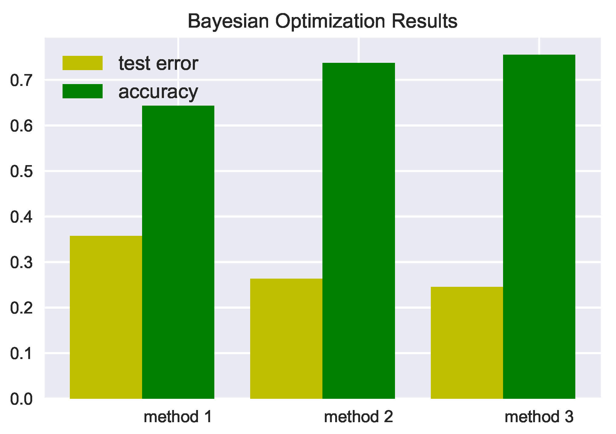
Statistic-base + wavelet-based features (method 1)0.3570.3570.1930.52264.3%
HOC-base features (method 2)0.2630.2630.1190.40773.7%
Statistic-based +
Wavelet-based + HOC-based
features (method 3)
0.2450.2450.1010.38875.5%
Table 5. Summary of findings.
Hypothesis NumberDescriptionAccepted/Rejected
H1The bio-sensor data from experienced experts can be distinguished from the biosensor data from studentsAccepted
H2The stress levels obtained from the bio-sensor data show a correlation to the NASA-TLX rating resultsAccepted
H3Compared to the novices, the experts feel less stress during a navigation taskAccepted
Publisher’s Note: MDPI stays neutral with regard to jurisdictional claims in published maps and institutional affiliations.

