1. Introduction
Concerns over climate change as well as the dwindling resources of fossil fuels have made experts replace renewable energy sources more than before [
1,
2,
3,
4,
5]. Therefore, the recent years have seen a rapid climb in the number of renewable energy-based power plants. Among all types of renewable energy resources, wind energy plays a crucial role in technical and economic approaches. Over the recent years, wind energy has become a promising alternative renewable resource for fossil fuels [
6,
7,
8,
9,
10]. In this regard, wind farms or wind power plants have been developed all over the world to utilize this cost-effective energy source even in remote areas with high potentials [
11,
12,
13]. The applications of wind energy are growing rapidly. However, there are still some challenges facing these applications. The main issue associated with wind energy is that the actual power generated by wind farms is less than its theoretical power capacity due to the wake effect, wind velocity variations, angle variations, wind turbine inefficiencies, and transmission line problems [
14,
15,
16]. The wake effect can be characterized as wind speed reduction and turbulent flow creation downstream of wind turbines [
17,
18,
19,
20]. As a result, this impact can reduce power generation by 10–20%. An enhanced layout of wind turbines can significantly improve power output and reduce its associated charges [
14,
21]. The power generated in a wind turbine is related to the perfect square of the receiving wind speed. Thus, the wind speed reaching each turbine is preferred to the extent its maximum. Nevertheless, the wind speed reaching downstream turbines is reduced in magnitude, causing a sharp drop in power generation of those turbines (as they are being under the wake effect of upstream turbines). Therefore, the layout of wind turbines should be arranged in a way to minimize the impact of the wake effect. This procedure is known as wind farm layout optimization (WFLO) [
22,
23,
24,
25,
26]. By doing so, the generated power from each turbine can reach a maximum value with lower associated costs.
The first priority in constructing a wind farm is to find a proper location [
25,
27,
28,
29]. This is due to the scarcity of lands and shortage of capital [
30,
31,
32]. Consequently, wind turbine positioning comes next. As a result, to harness the highest possible power from a certain power plant, a comprehensive assessment on the placement of wind turbines should be taken into account. Wind farm layout optimization is a crucial subject in wind energy literature [
33,
34,
35]. At this point, numerous researchers have been concentrated on the WFLO problem [
16,
36,
37,
38].
Patel [
39] stated that in designing a wind farm layout, appropriate distances between wind turbines should be estimated. According to Patel’s study, the optimal arrangement is in rows of 8–12 rotor diameters separately along the wind direction and 1.5–3 rotor diameters apart along the crosswind direction. One of the first research attempts for optimizing a wind farm layout was made by Mossetti et al. [
40]. By using the genetic algorithm, they minimized the objective function value, which was the unit cost per power production. They implemented a simple, empirical cost model. In 2013, Samorani et al. [
41] underlined the importance of the optimization of wind farm configurations involving optimally placement of wind turbines to diminish the wake effect. This problem has drawn the attention of the scientific community. However, existing approaches are not fully responding to the needs of wind farm developers, mainly since they do not usually address the challenges associated with construction and logistics. Eroğlu et al. [
42] used a particle filtering approach to achieve an optimal layout of a specific wind farm. The boundary of the wind farm and distances between turbines were regarded as two main constraints. The results indicated that the particle filtering approach can compete with the ant colony and evolutionary strategy algorithms. Chen et al. [
43] investigated the effect of using wind turbines with different hub heights on the overall output power. The nested genetic algorithm was used to analyze three different wind conditions. The results of this study demonstrated that by using different hub heights of wind turbines, power generation increased (compared with a wind farm having the same number of turbines). Shakoor et al. [
44] proposed a novel method called definite point selection (DPS) that could find the optimum placement of turbines. The DPS method was approved to be more effective than the earlier proposed methods. Gao et al. [
22] presented a 2D analytical wake effect model based on the Jensen’s wake model and Gaussian function. In this study, wind farm efficiency dropped to 77.83% from 96.83% for a collection of 38 wind turbines within a large wind farm. Wang et al. [
45] addressed more complex wind farm boundaries by which a new constraint handling method was introduced. This study stated that the unrestricted coordinate method, under the sequential land plot scenario, generates optimal outcomes, with the lowest energy cost and highest efficiency. Parada et al. [
46] used the Gaussian wake model to calculate wind speed loss. In this study, the cost of energy was optimized by the genetic algorithm. They asserted that the use of a more robust wake model in the WFLO problem did not lead to greater efficiency in real wind farm cases.
Sun et al. [
47] adopted a conceptual 2D wake model to calculate wind losses caused by the wake effect. In this study, the cost of energy (COE) was used as a criterion to compare the effectiveness of this novel method. The results indicated that the optimization method used in this study can reduce the COE down to 1.02 HK
$/kWh.
Vasel Behagh et al. [
48] studied the effect of height optimization of turbines on the annual energy production (AEP). In this study, they compared two wind farms with an equal number of turbines (also similar types and positions). In one wind farm, all turbine heights were identical, while the other one had alternating rows of tall and short wind turbines. The results exhibited that the vertically staggered configuration generated more power output by 5.4%. Hou et al. [
49] proposed an optimization technique for offshore wind farms. In this study, they attempted to find the optimized layout of turbines in order to achieve maximized power generation. The PSO algorithm with multiple adaptive methods (PSO-MAM) was used as an optimization algorithm. The results of this study indicated that the aforementioned method can suggest a layout that increases the power output by 3.84%. Tian et al. [
50] investigated the optimal tip speed ratio and pitch angle for wind turbines by an exhaustive search (a brute-force search). A solution for this problem was introduced considering the estimation error of the wake model, which was to yield the optimal control curves for each wind turbine. In that study, the annual energy production was increased by 1.03%. Mir Hassani et al. [
51] studied the effect of using different hub heights on the total power generation of a wind farm. They presented a mathematical model for wake effects considering wind turbines with different hub heights as well as a new optimization model. Abdelsalam et al. [
52] aimed to optimize a wind farm layout by the binary real coded genetic algorithm (BRCGA) based on a local search (LS), gathering robust single wake models with suitable wake interaction modeling. The model used in this study was the Jensen wake model alongside the sum of squares model.
Kirchner-Bossi et al. [
53] introduced a new technique for wind farm layout problems using the Gaussian wake model. This methodology was applied to two real wind farms and was also compared with the Jensen model. Stanley et al. [
54] optimized some wind farms using a coupled optimization method. The coupled optimization led to a reduction in the cost of energy by 2–5% compared to sequentially optimization of wind farms with turbine spacing of 8.5–11 rotor diameters. Some of the wind farms in that study also exhibited an additional 10% reduction of energy costs.
Pratt et al. [
55] compared several wake effect models using analytical and CFD methods for a wind farm at Block Island. The results showed that a value in the higher range of the examined WDC (0.06 and 0.07) and TI (12% and 14%) values represented a better comparison to the observed data. Diaz et al. [
56] developed the actuator disc (AD) model which was the most common simplified wind turbine model, based on the Open FOAM open-source software. Results demonstrated that values for low and high wake impact situations were improved with 2.5% and 1.3%, respectively. Patel et al. [
57] introduced a novel method called the geometrical pattern-inspired placement methodology to find the layout of turbines with maximum total power output at Kutch-India. The enhanced passing vehicle search (PVS) algorithm was used in this study. The results showed that the power output was improved by 4.29%.
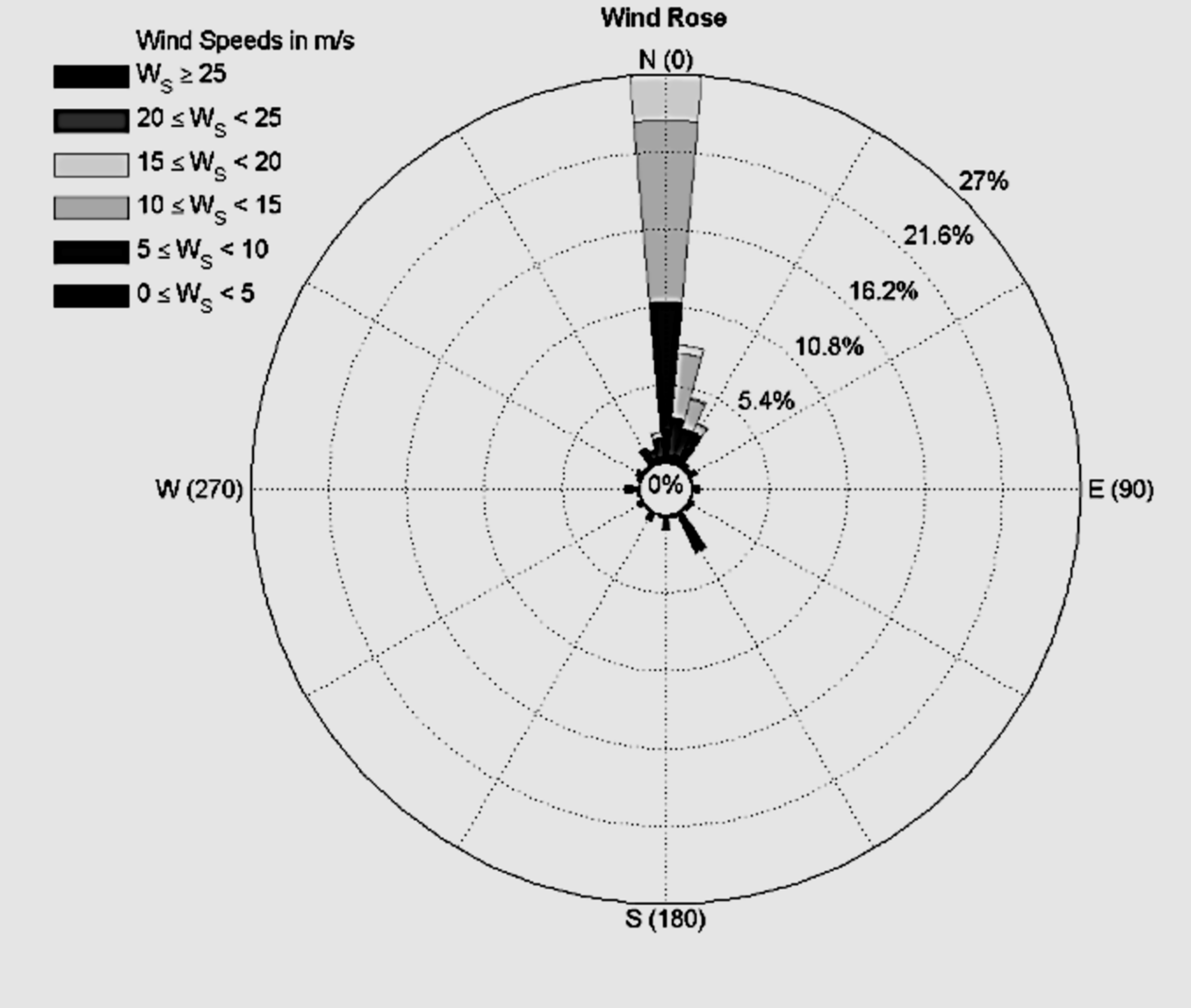
The purpose of this original research is to optimize the 3D layout of turbines at the Valfajr Wind site in Manjil, Iran. In other words, this is an attempt to identify the best placement of turbines and their heights as the power plant reaches its optimal operating level [
58]. Initially, by considering the wind and geographic information of the region, the wake effect is analyzed with the Jensen method [
59,
60]. Next, the objective function, which is the cost of total power generation [
40,
61,
62], will be estimated. Finally, the objective function will be optimized using the particle swarm optimization algorithm.
2. Materials and Methods
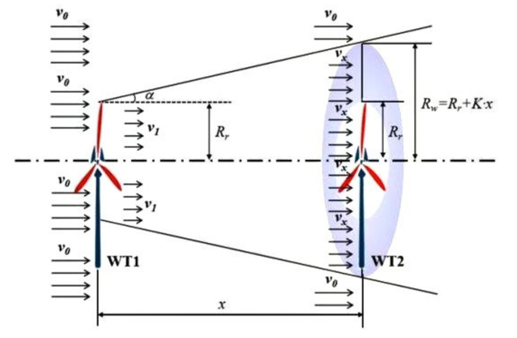
In this study, the Jensen’s method is used to model the wake effect. As shown in
Figure 1, when wind passes through a rotor blade, its speed falls and the waking zone spreads from the wind flow, similar to a cone [
63,
64,
65]. The radius of this cone can be calculated.
As shown in
Figure 1, if the wind turbine zone is located downstream of the wake cone, the wake and the downstream turbine will overlap. In case the region is generated by an upstream wind turbine, the wind speed will experience reduction [
6,
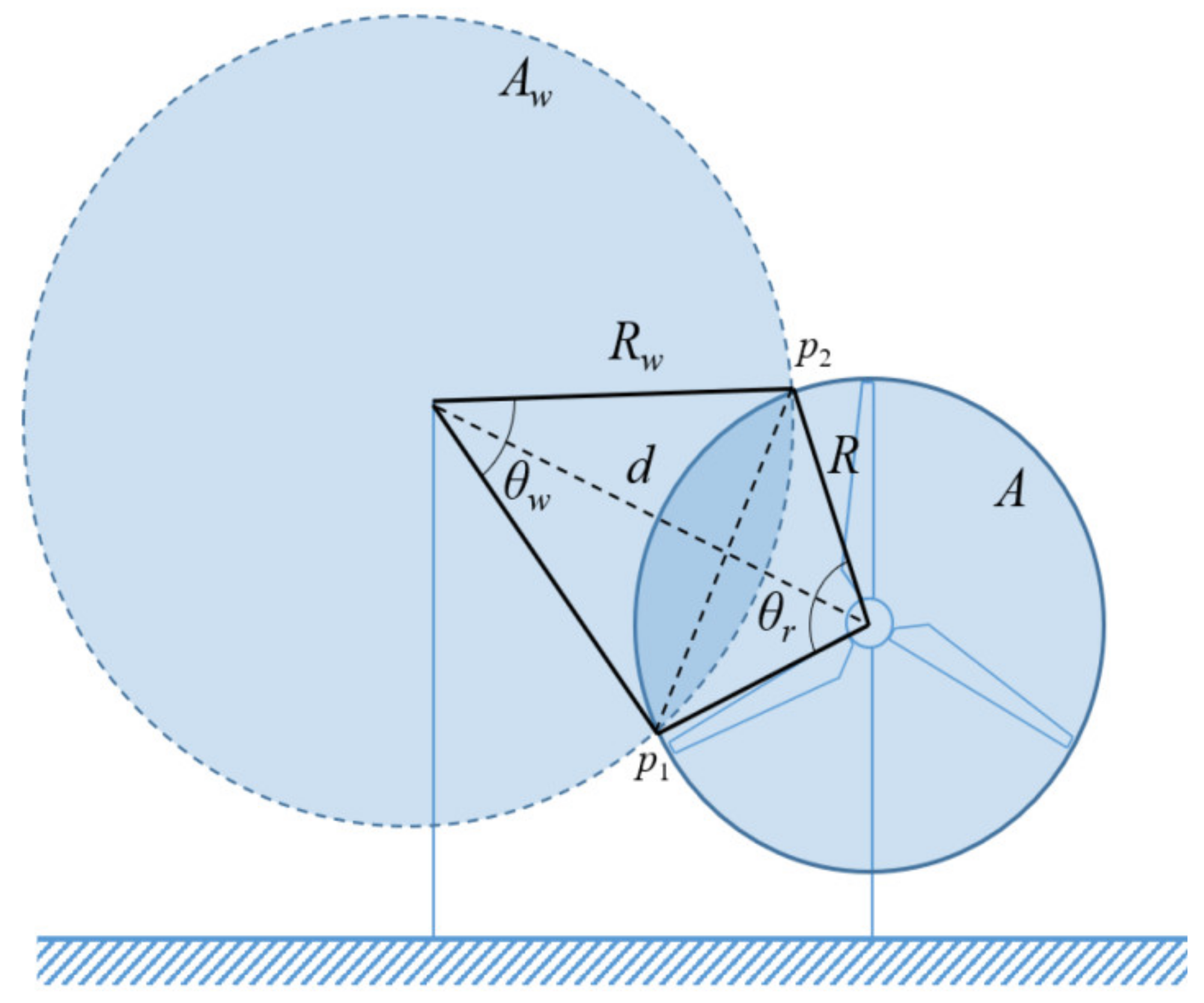
66]. Additionally,
Figure 2 presents the wake shadow area.
In the above equation,
is rotor’s radius,
. is the distance of turbines, and
is the expansion rate that takes a value between 0.04 to 0.08 which is calculated by [
67,
68]:
where
is the hub height and
is the roughness length. Wind flow velocity of the wake is computed as [
69,
70]:
where
is the area created by the rotor blade system and
refers to an area covered by the downstream turbine and the shaded area of the upstream turbine, which is calculated by Equation (4) [
71]:
For calculating wind speed originated from multiple upstream turbines reaching a downstream wind turbine, the following equation is used (Equation (5)):
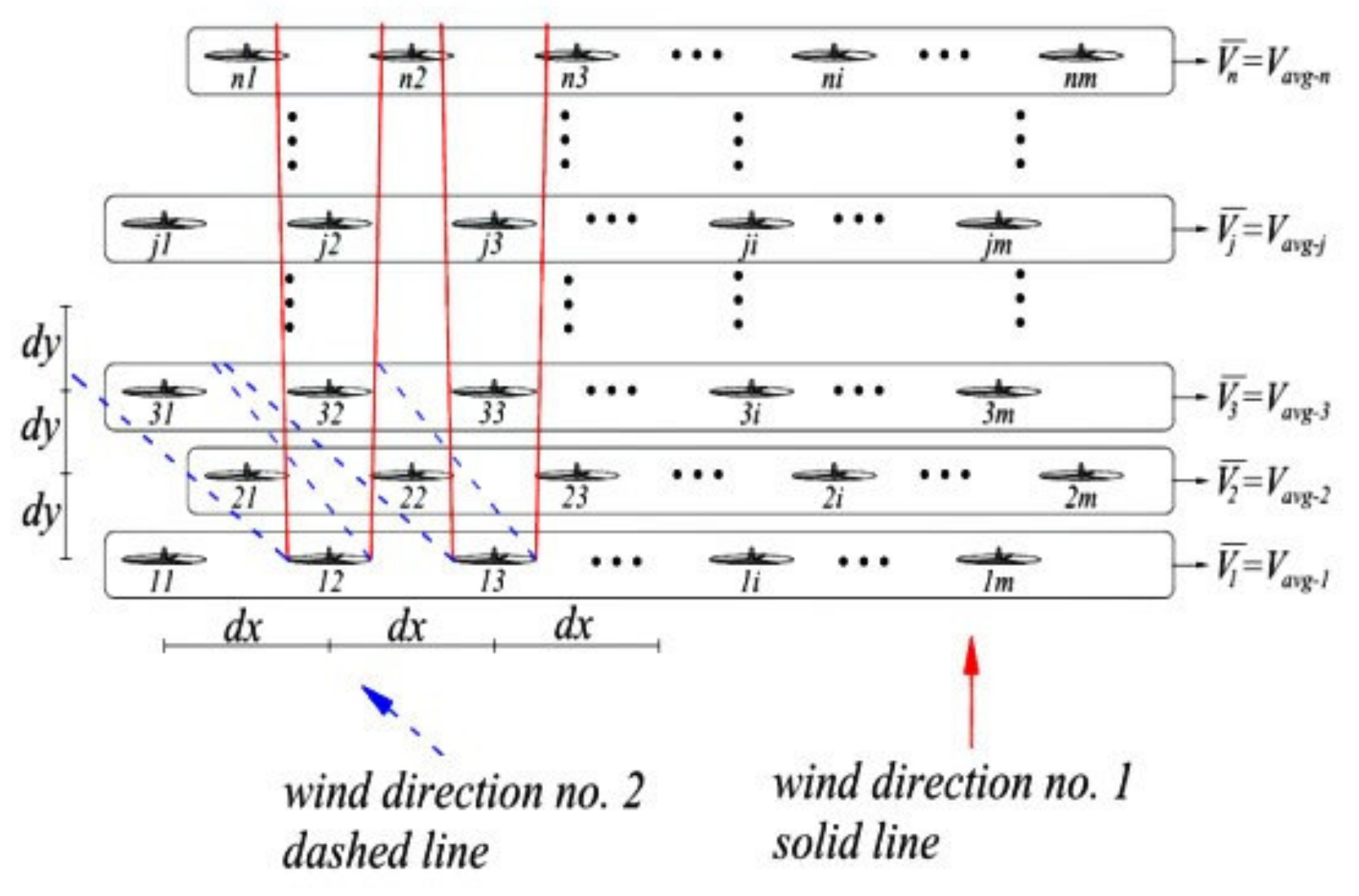
Shaded wind turbines and the number of shaded units are different and they both depend on the wind direction and the geometrical layout of wind turbines. It is illustrated in the following figure for two different directions of wind. As shown in
Figure 3, the area covered by the vortex cone changes with wind direction [
51].
The wake factor can be defined as [
37,
72]:
which can be formulated as:
where
is the number of turbines in a row,
is the number of rows, and
is the wind speed fraction perpendicular to the
i-th turbine in the
j-th row. In addition,
stands for the power generated by a turbine with wind speed of
. When the wake factor is equal to one, it means there is no wake effect.
The following relation is used to obtain wind speed at any hub height [
66,
73]:
where
represents the reference wind speed and
is the roughness length.
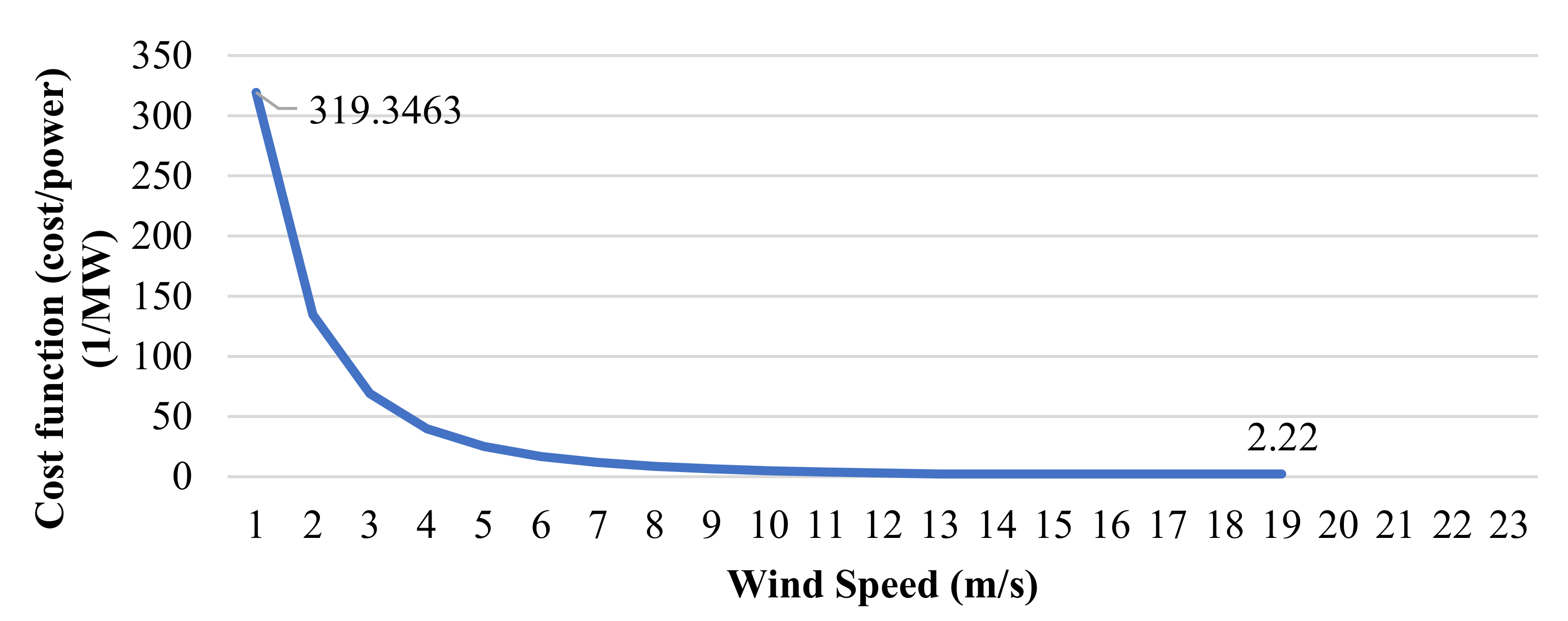
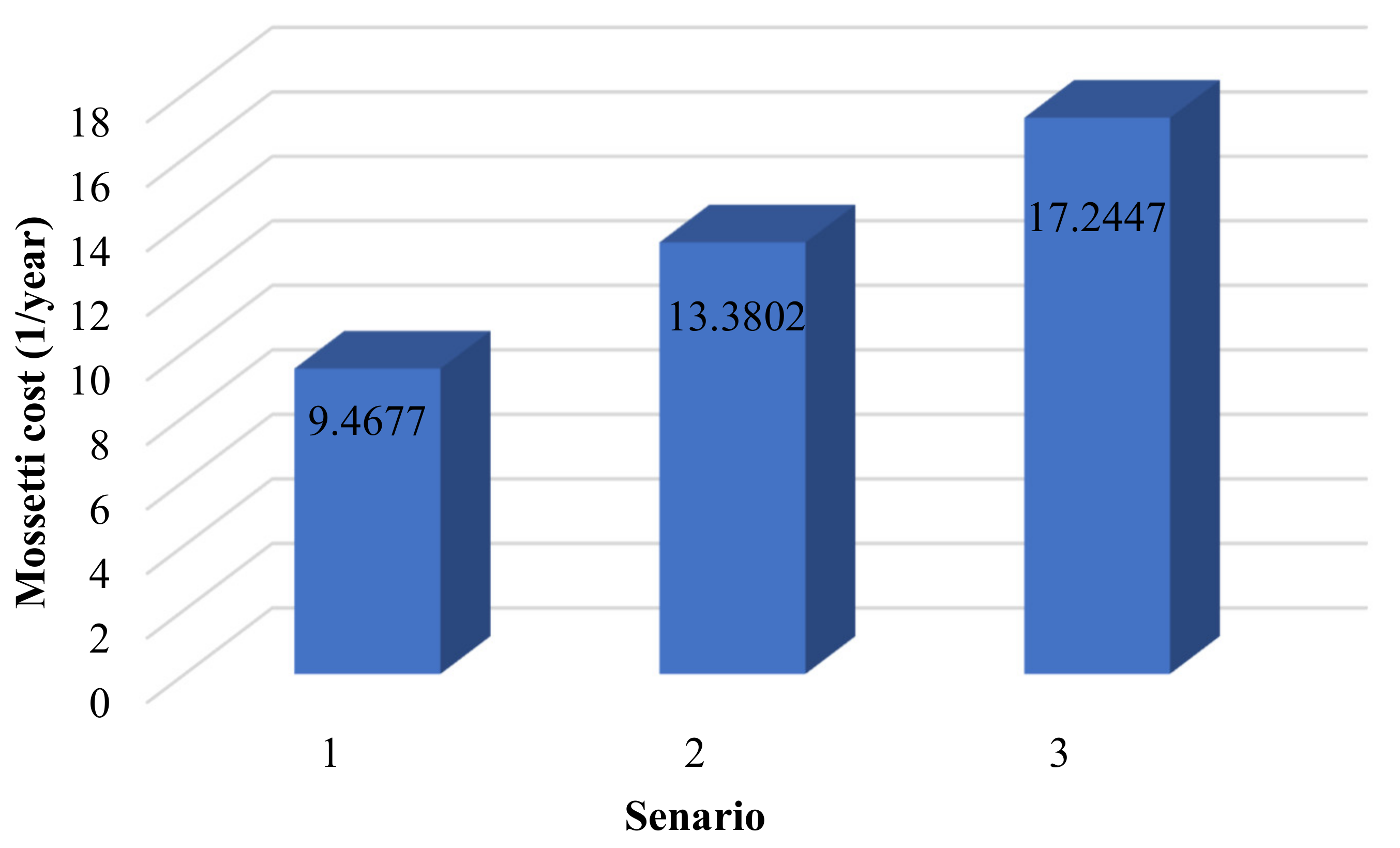
The cost function considered in this study is the same as Mossetti et al. [
40]. Through this function, the annual plant’s total cost by using the number of turbines (
) can be calculated with decent accuracy.
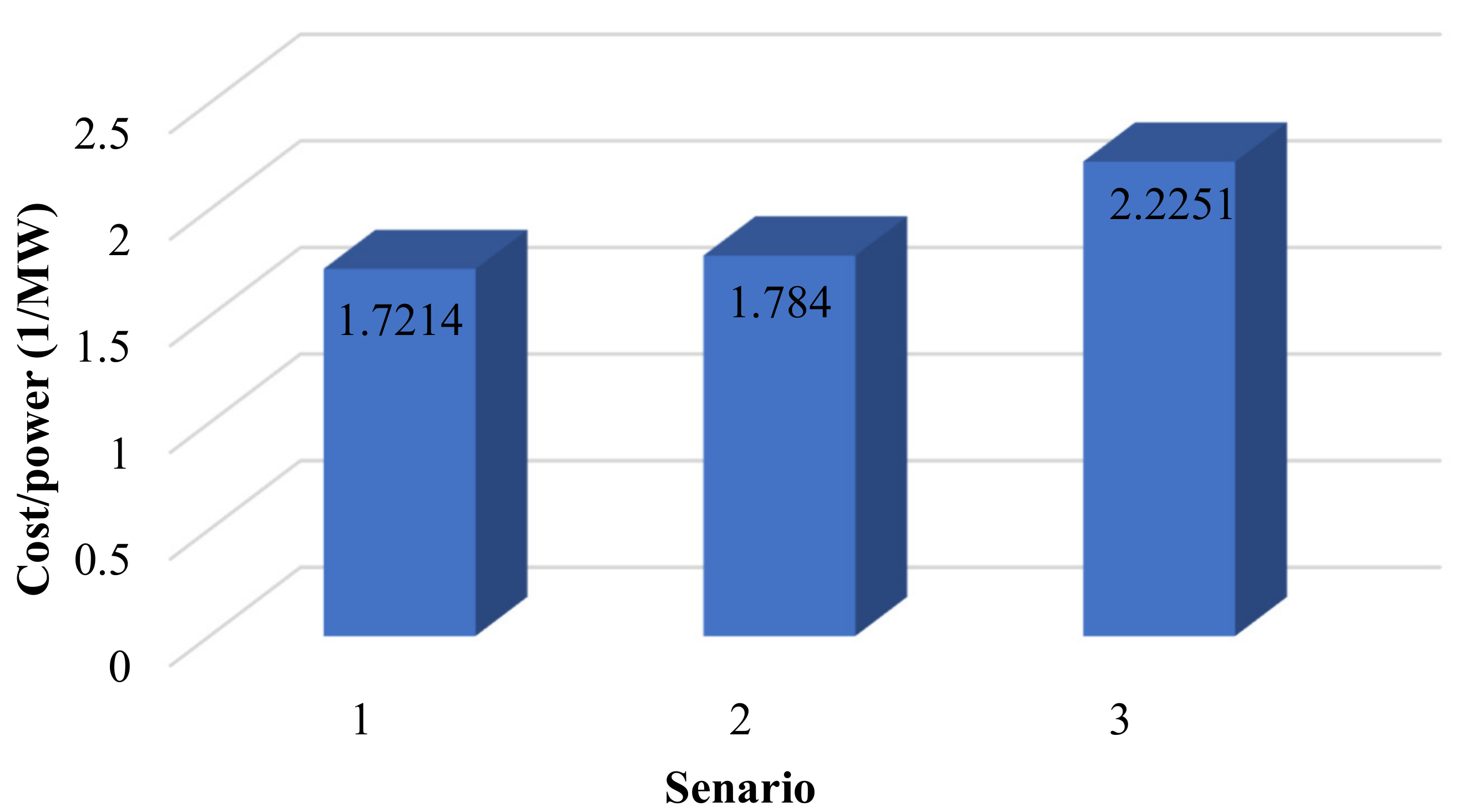
The objective function for the optimization problem in this study is defined as:
where
stands for the total power generation in the wind farm and can be calculated as:
where:
where
is air density,
is the rotor radius,
is wind speed, and
is the power coefficient of the wind turbine.
3. Particle Swarm Optimization
In this research, particle swarm optimization is used to optimize the objective function. Due to the appropriate and adapted nature of the algorithm to achieve an optimal solution, the algorithm has fast speed [
4,
66].
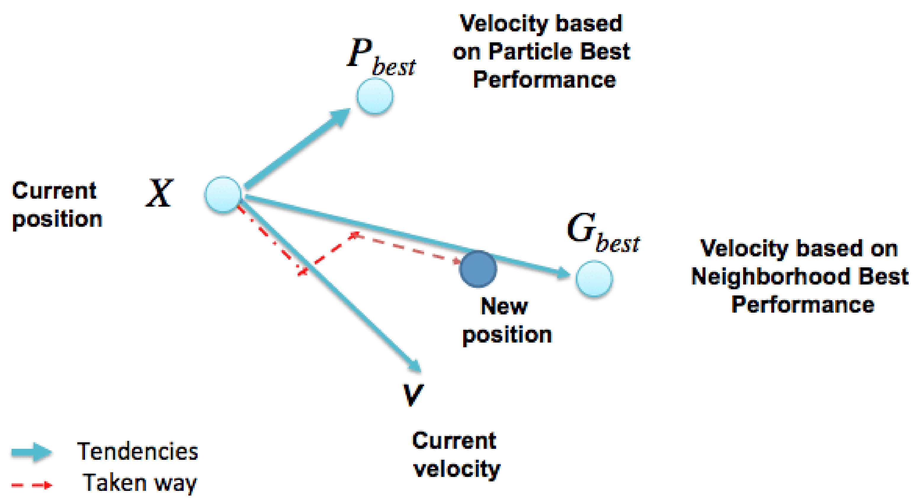
Figure 4 indicates the motion pattern in the particle swarm algorithm.
In each step, the velocity of particles becomes updated from the following relationships:
In Equation (13), is the inertia weight factor which indicates the effect of the iteration speed vector on the velocity vector in the current iteration , is the constant learning coefficient moving in the direction of the best personal particle value, is the constant learning coefficient moving along the path of the best particle found among the entire population, and with are two random numbers with uniform distribution from 0 to 1.
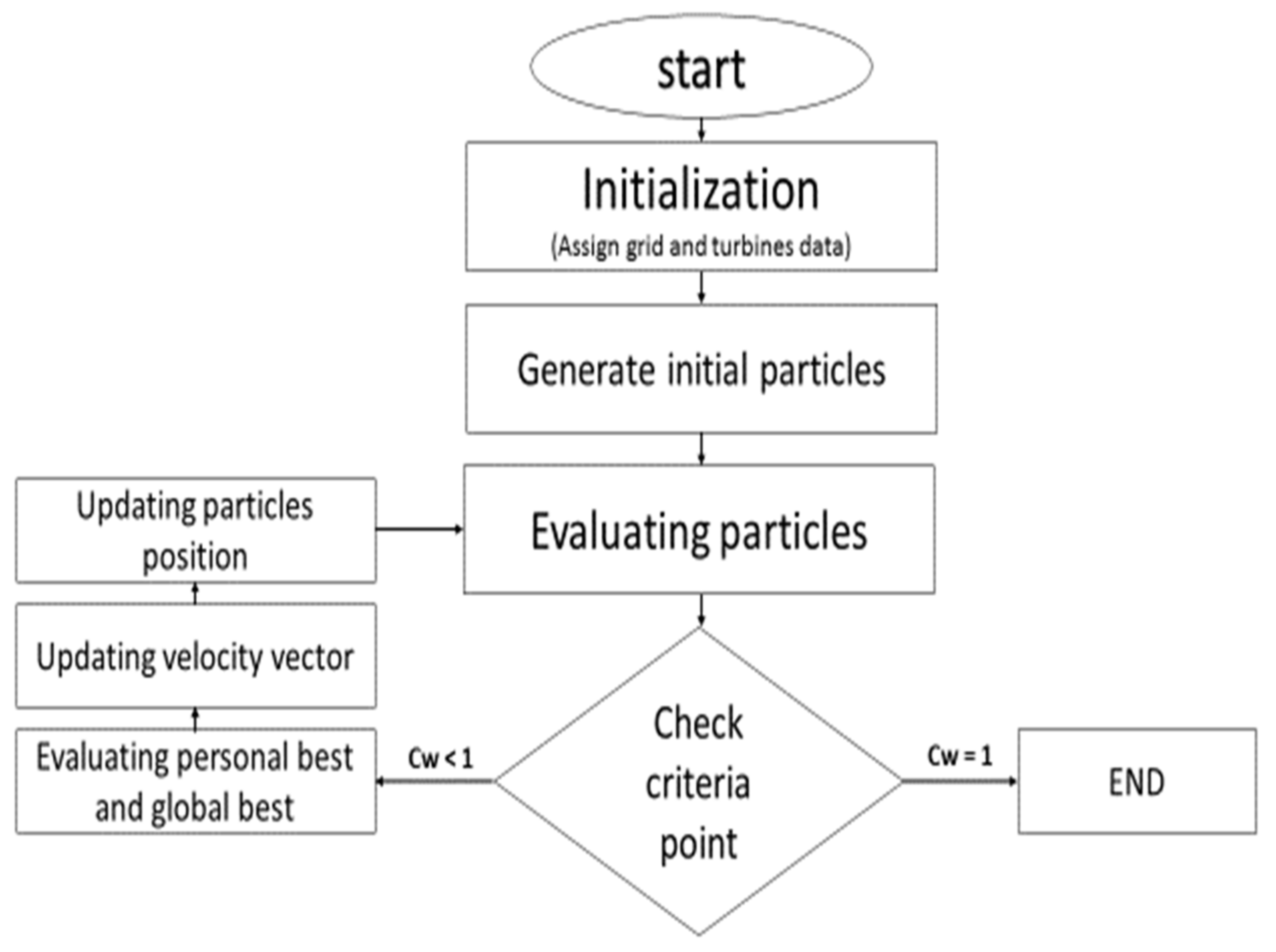
Steps of the Implementation of the Particle Swarm Algorithm
(1) Random production of particles: the stochastic production of the initial population is simply the random assignment of particles with uniform distribution in the solution space.
(2) Purpose of the objective function: At this stage, each particle representing a problem-solving must be evaluated. Depending on the provided equation, the evaluation method will be different.
(3) Recording the best location for each particle and the best position among the whole article: at this step, the amount of target function obtained for all particles is compared with the best amount of cost obtained for each particle.
(4) Updating the speed vector of all particles: after calculating the best particle for each this method, the velocity vector available for each particle is updated by the best position of each particle, the current position, and the best position among all particles.
(5) Convergence test: There are various methods for investigating the algorithm. For example, a certain number of iterations can be found from the beginning. Another method often used for convergence test of the algorithm is that if there is no change in the value of the best particles in a sequence of consecutive iterations, then the algorithm ends.
7. Conclusions
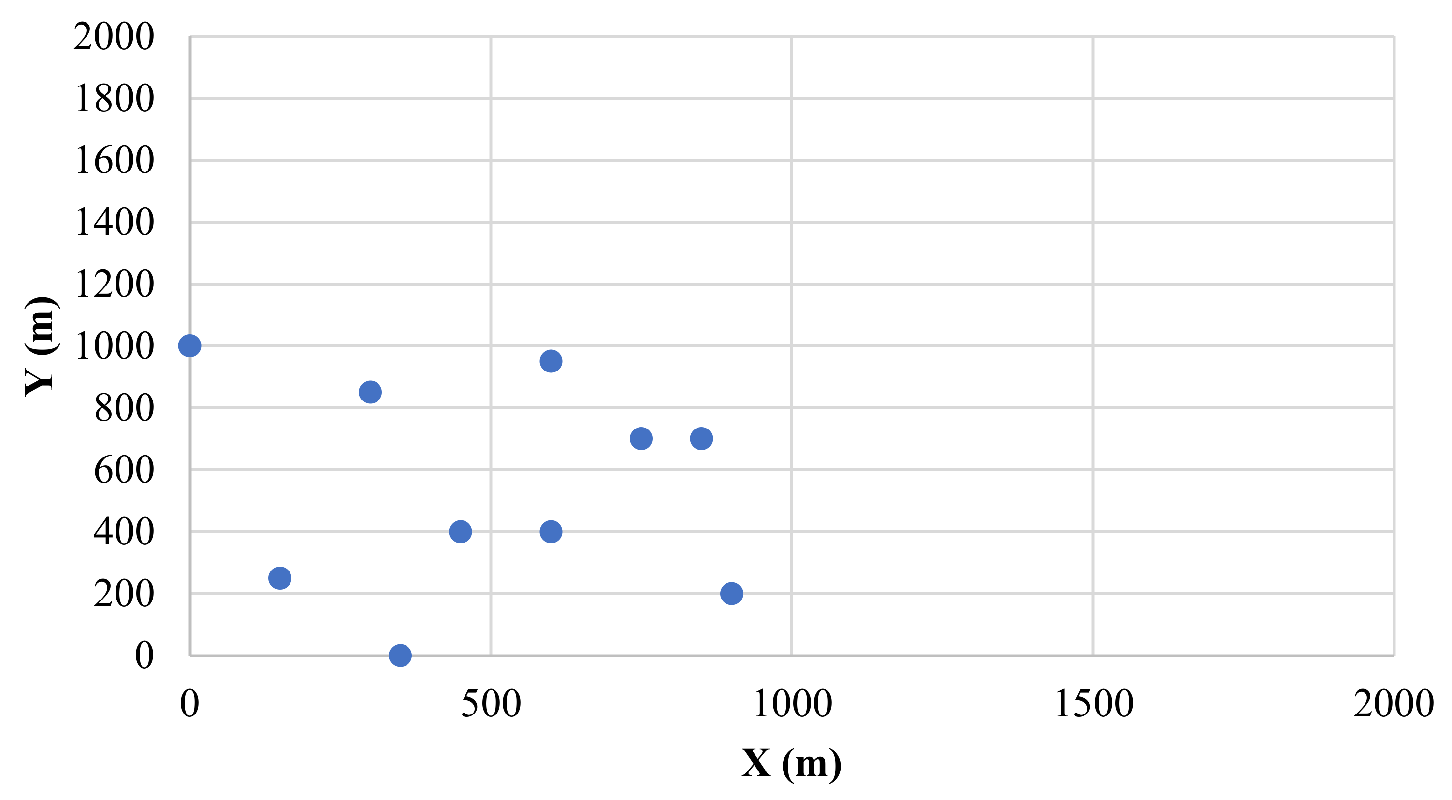
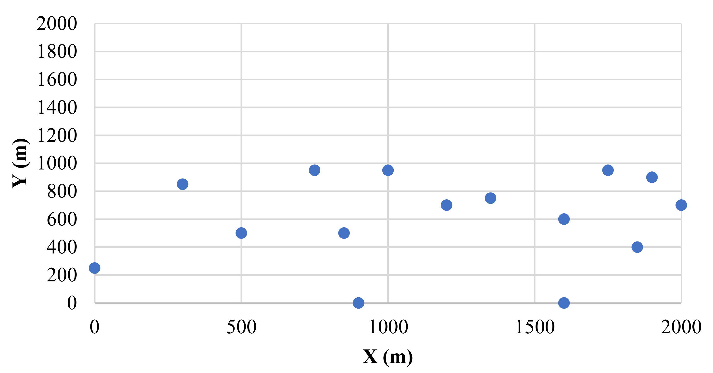
The total power generated by wind farms is smaller than their theoretically calculated output. This is mainly because of the wake effect. In order to increase the actual output power of wind farms, the existing wake effect should be minimized. This puts a premium on the placement of wind turbines. In this study, the Valfarjr site of Manjil wind farm’s layout is optimized in 3-D. In other words, wind turbine positions, wind farm configuration, and heights have been selected to be optimized in order to minimize the wake effect. Firstly, by considering the regime of wind and geographic data of the region, the wake effect is modeled by the Jensen’s method. After that, the objective function, which is the cost to energy output, is calculated according to the method proposed by Mossetti. In the end, the objective function is optimized by employing the particle swarm optimization algorithm.
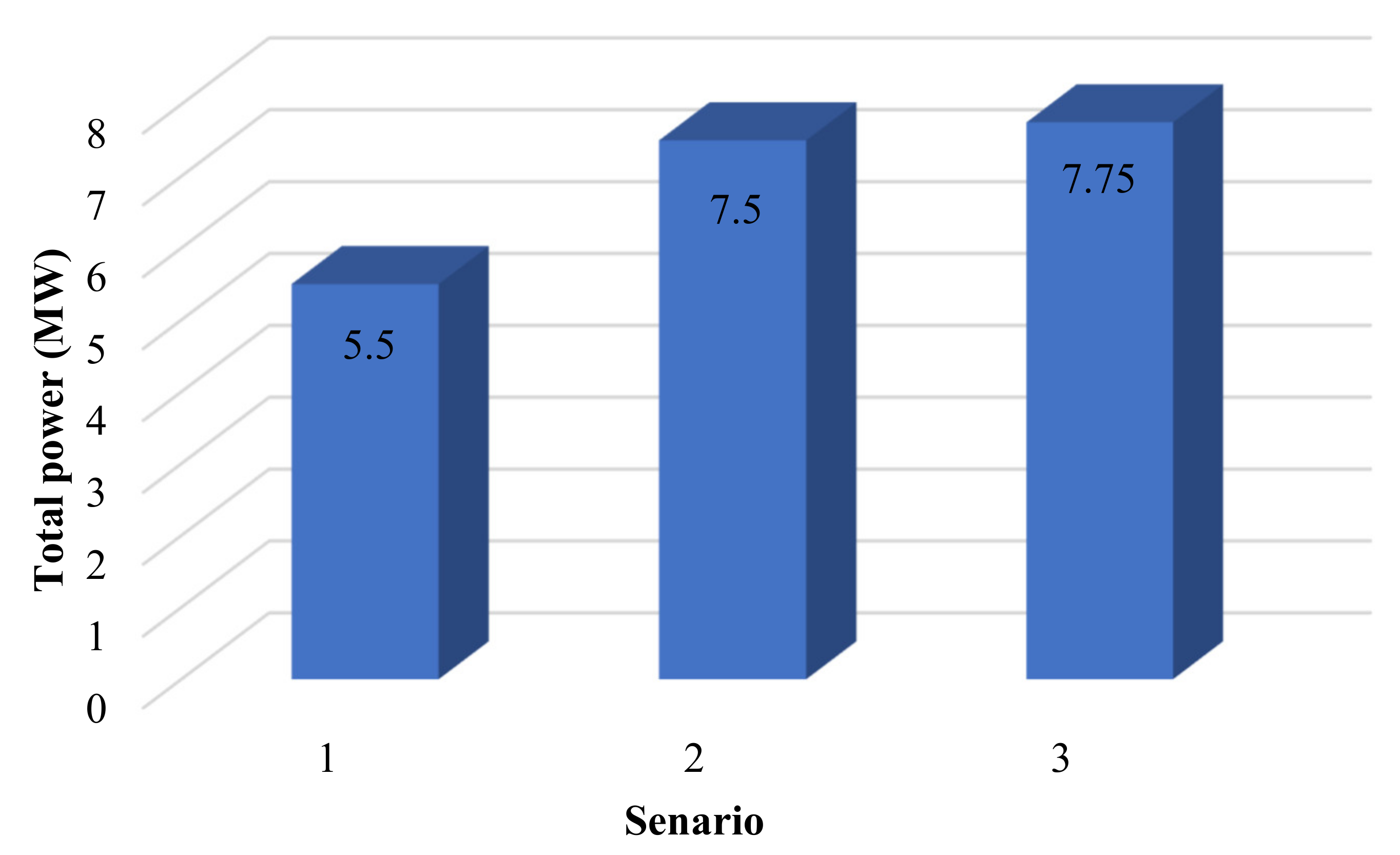
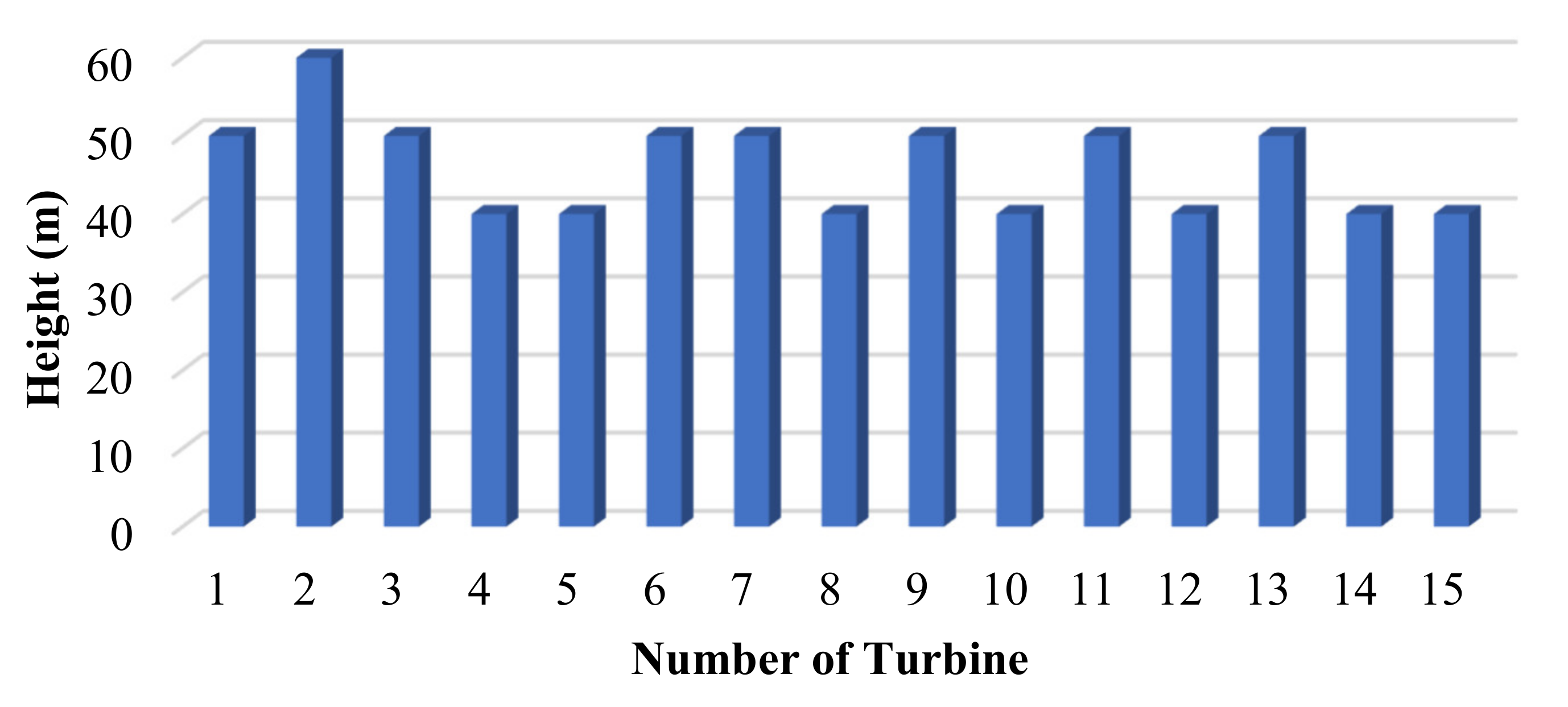
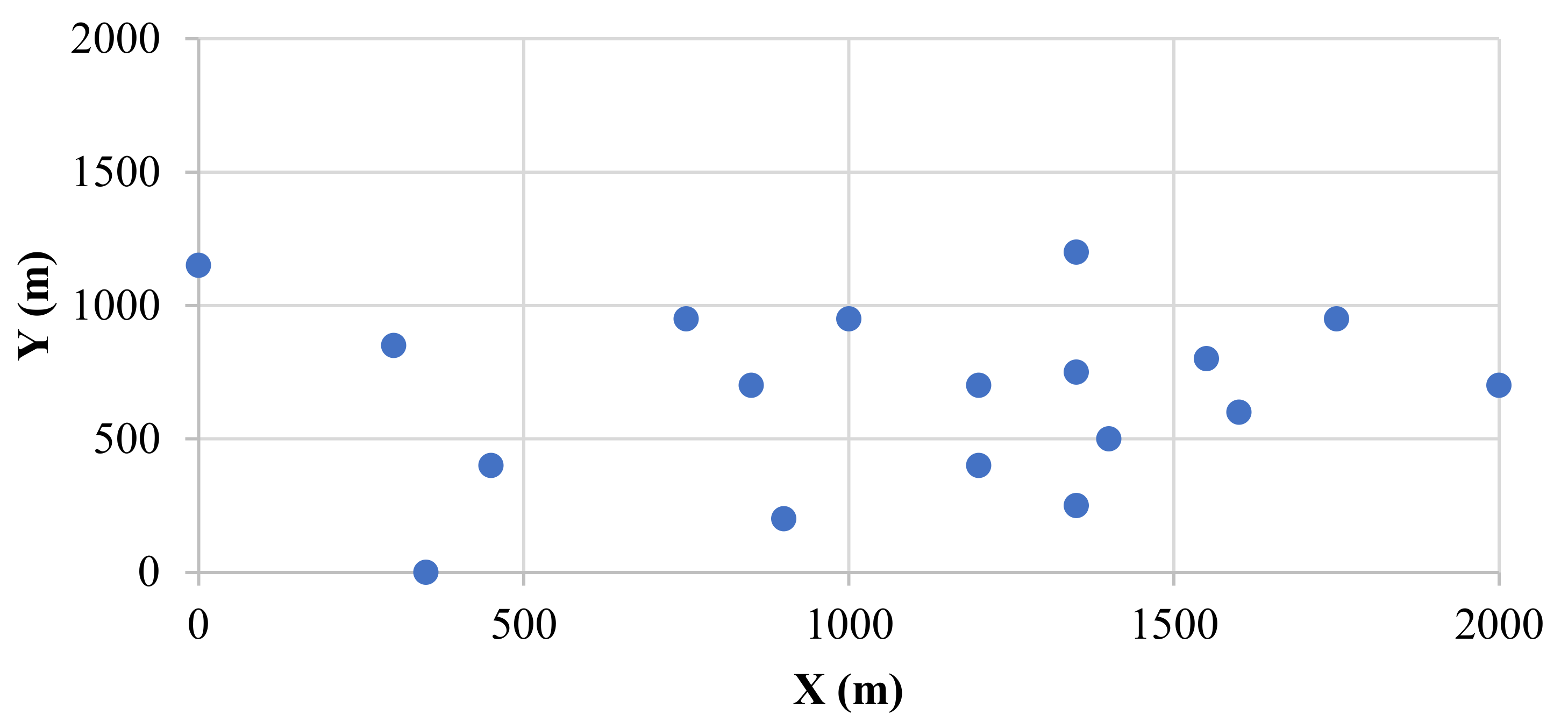
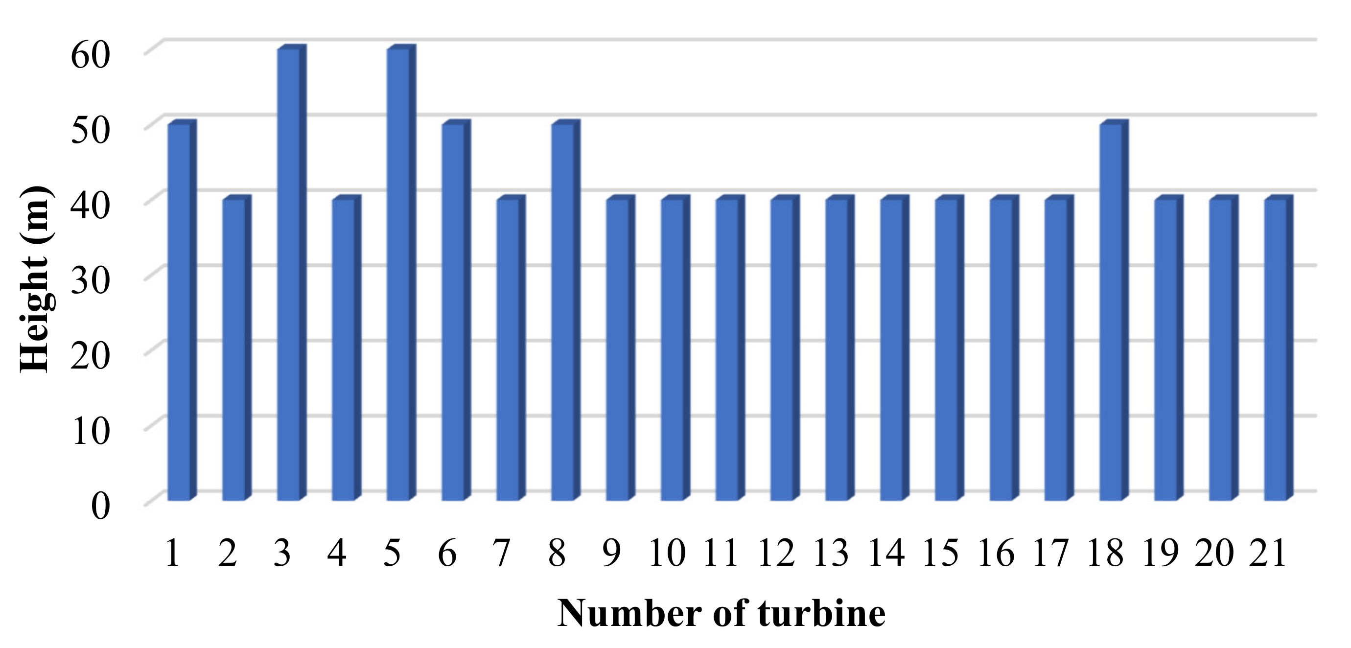
By setting optimal turbine coordinates, power generation increased by 10.75% and decreased the cost by 9.42%. Moreover, by using 15 turbines of 500 kW, installed in optimal positions and heights, power generation decreased by 3.22%, while the cost decreased by 20%.
For future studies, the economic aspect of the plant by using different economic methods could be investigated. Moreover, to achieve more accurate results, turbulent flow impacts can also be scrutinized.


 ,
, 


