Cyclostationary Approach to the Analysis of the Power in Electric Circuits under Periodic Excitations

Abstract

This paper proposes a cyclostationary based approach to power analysis carried out for electric circuits under arbitrary periodic excitation. Instantaneous power is considered to be a particular case of the two-dimensional cross correlation function (CCF) of the voltage across, and current through, an element in the electric circuit. The cyclostationary notation is used for deriving the frequency domain counterpart of CCF—voltage–current cross spectrum correlation function (CSCF). Not only does the latter exhibit the complete representation of voltage–current interaction in the element, but it can be systematically exploited for evaluating all commonly used power measures, including instantaneous power, in the form of Fourier series expansion. Simulation examples, which are given for the parallel resonant circuit excited by the periodic currents expressed as a finite sum of sinusoids and periodic train of pulses with distorted edges, numerically illustrate the components of voltage–current CSCF and the characteristics derived from it. In addition, the generalization of Tellegen’s theorem, suggested in the paper, leads to the immediate formulation of the power conservation law for each CSCF component separately.

1. Introduction

Modern hardware systems performing digital signal processing can easily reach high complexity, since they typically consist of many specialized devices. In turns, the majority of these devices are assembled from a variety of electronic components, in which electric currents and voltages play the primary role in the description of phenomena at the physical level. For instance, one of the typical issues solved in the electromagnetic compatibility framework [1] is the detection of potential sources of interference, which may affect the stable work of the entire device or even neighboring devices. A traditional and easy to understand model describing the property of components can be built as an electric circuit being assembled from lumped elements only or lumped elements properly combined with parts of transmission lines.

The proper choice of an appropriate model is mainly based on two points. The first one is the primary role of the component, i.e., whether it is intended to be an antenna, microstrip line, connector, frequency selective filter, or the input port of an embedded integral circuit. The second point is determined by a certain relation between the spectrum width of the processed signals and the passband (or passbands) of the analyzed component. Thus, in the case of digital signal processing, where the spectrum is considered to be concentrated in a baseband with respect to the lowest resonant frequency range, the component’s electric property can often be modelled as a simplified RC circuits [2]. However, if the resonance behavior cannot be neglected, a more accurate model, exhibiting weak resonant properties, may well be introduced by means of a generalized resonant circuit, either of parallel or serial type, with relatively low Q factor, typically not exceeding the value of 2.

In an ultrawideband case, where the signal spectrum spreads over a frequency band covering several natural electromagnetic modes of the component, the appropriate model has to be reconsidered. The simple approach to enhancing the lump-element model consists in combining multiple resonant circuits [3]. However, this can be performed accurately only if the component possesses sharp resonances; otherwise, such a model will be nothing but an approximation technique, which can be developed further, to surrogate models [4]. An alternative approach proposes the extra inclusion of an idealized transmission line, while the lumped element remains the resonant circuit [5]. Models of this type showed high performance in cases where the natural resonances are rather smooth or the introduction of transmission line can be proved with geometric or physical reasoning [6].

Although the normal operating mode of signal processing devices suggests periodically processing structured signals with random information components [7], deterministic periodic signals will inevitably be present. Moreover, during the verification phase, a device can be switched to a special mode, where the processed signals are to be changed to satisfy predetermined sequences, forming patterns inheriting the true periodical structure.

At first glance, the accurate analysis of power in the elements of low Q circuits does not seem to be difficult. However, this problem turns out to be challenging when it comes to the excitation by electric currents or voltages described by arbitrary periodic waveforms. Thus, in modern university level textbooks devoted to engineering circuit analysis, e.g., those authored by Hayt [8] or Irwin [9], the topic of power analysis in electric circuits is generally taught in an ambivalent manner. In the beginning, instantaneous power tends to be introduced as a time-varying function that is a product of the voltage across, and current through, an element or extracted one port within the analyzed circuit. Next, the average power evaluation is shown for a case in which the circuit is in a steady state mode caused by constant or periodical excitation by its sources. However, in the case of the sinusoidal waveform, an alternative concept of the power analysis is rather suddenly offered, bringing to life such terms as effective values, reactive, apparent and complex power, power factor and power triangle. Although this concept serves well for describing a single frequency sinusoid, formidable obstacles emerge as soon as one attempts to apply a coherent generalization to arbitrary periodic waveforms.

The law of instantaneous power conservation in an electric circuit, which is often referred to as Tellegen’s theorem [10], is the electrical engineering adaptation of a more fundamental energy conservation law. It was explained in [11] that a balancing equation, due to Tellegen’s theorem, will remain valid after such transformations of the currents and voltages in the entire circuit that do not violate Kirchhoff’s laws. The representation of the varying power in the time domain, with an attempt at building a model with a clear physical meaning, is presented in [12]. The direct implementation of balancing instantaneous power is given in [13].

The second of the above mentioned power concepts is based on the theory proposed by Budeanu [14], and its main points are thoroughly discussed in [15], where it is compared to an alternative power decomposition suggested by Fryze [16]. Some additional arguments in favor of the latter were also added in [17].

Budeanu’s methodology has been dominant for the past century due to its relative simplicity, and has become extremely popular with electrical engineers dealing with sinusoidal waveforms. In particular, those engineers who are working within power delivery systems have developed a specific professional viewpoint on the topic, e.g., [18]. A possible way to generalize Budeanu’s theory consists in finding a proper definition of reactive power. This definition must preserve the applicability of the concept to the case of an arbitrary periodic waveform. Moreover, such a definition is expected to have some physical meaning and, which is also important, obey some conditions, e.g., the power conservation law.

The most prominent approaches being researched recently are based on functional space decomposition used for extracting so called power components. Examples are the vector space decomposition for reactive power presented in [19], the hyperspace decomposition in [20], and the more general geometric algebra approach proposed in [21]. All three show different ways of expressing partial power components. The third one appears to be developed further, into the multivector representation [22]. An attempt at power analysis using a basis different from a harmonic series was made in [23], in which the Haar wavelet was considered as a possible candidate.

Among other possible approaches, there is the conservation power theory [24], which is originally based on the decomposition carried out in the time domain [25]. Despite the fact that this theory is gaining popularity, it was criticized in [26,27] for its lack of a clear physical meaning and misguiding conceptualizations, such as energy taking on a negative value.

The further development of Fryze’s ideas, which was carried out by Czarnecki [28], has led to Currents’ physical components theory. The concept considers the current flowing through a one port as a sum of three components: active, reactive and scattered. They are in charge of instantaneous power distribution between three pairwise orthogonal components. Some arguments in favor of this theory were also discussed in [29].

In contrast to other approaches developed so far, this paper offers an alternative method for power analysis based on the theory of cyclostationarity (CS). The history of the focused investigation of CS phenomena spans about 65 years, starting from the pioneering works written by Bennett [30] and Gladyshev [31]; the latter called such random processes periodically correlated. Having been originally introduced as a set of adhoc models describing so called hidden periodicity, over the last decades, CS signal analysis has matured into a selfsustaining branch of science, whose milestones and further trends are described, respectively, in [32,33]. The recently published comprehensive monograph by Napolitano [34] provides a contemporary, detailed explanation of the foundations and state of the art developments in CS analysis. Some introductory CS examples, yet in the analysis of mechanical systems, may be found in [35], where the vibration signals of rotating machines were analyzed with advanced spectral techniques [36].

As it follows from many sources, cyclostanionarity seems to be firmly associated with the concept of a second order harmonizable random process [37]. The ensemble expectation taken on its lag product varies in time and, more importantly, can be expressed as a periodic or almost periodic function [34]. Equivalent frequency representation can be given via the expansion into Fourier series, whose coefficients are functions dependent on the lag parameter. However, from a nonprobabilistic point of view, which is illuminated in book [38] by Gardner, even deterministic periodic waveforms can be treated as first order CS processes.

The goal of this paper is establishing the foundation of a novel method that aims at performing accurate and detailed power analysis of the elements of electric circuits under periodic excitation. The proposed method is based on complex Fourier series decomposition rather than either sine–cosine decomposition or a phasor representation of the harmonics constituting the periodic currents and voltages. Despite its formal complexity, CS analysis seems to be an extremely effective approach, since it helps to reveal elementary power components, obeying the conservation law. Such components can be directly used to the noncontroversial derivation of all other quantities typically exploited for power description.

This paper demonstrates how the standard collection of CS characteristics can be adapted to build an effective tool for describing the power in the elements of an electric circuit under the first order CS processes of voltages and currents. This collection includes the cyclic correlation function and spectral correlation function, which are widely exploited for coping with second order CS processes. The period of the processes is assumed to be known. In the case of unknown period, as often happens in practice, one can take on an appropriate period estimator prior to tuning the model parameters. Such a period estimator can be implemented via either synchronous averaging [39] with CS detection [40,41] or more promising techniques based on sample coherency analysis [42,43].

The rest of the paper is organized as follows. The second section presents the theoretical model of voltage–current two-dimensional cross correlation function (CCF), which appears to be a specific extension of instantaneous power. Next, the cross spectral correlation density is derived in an explicit closed form, which allows redefining the common quantities used in the power analysis directly from its components. The particular case of linear time invariant elements is also briefly explained in Section 2. In Section 3, the evaluation of the suggested characteristics is illustrated with numerical examples, where a resonant parallel circuit is excited by different periodic waveforms. The discussion in Section 4 considers the extension of the power conservation law that the components of the spectral correlation functions obey. The paper ends with conclusions.

2. Theory and Models

2.1. Voltage, Current and Instantenious Power Definitions

The instantaneous power delivered to any element in a circuit is considered as a time-varying signal given by the product of the instantaneous voltage v(t) across the element and the instantaneous current i(t) through it:

$$p(t)=v(t)i(t).$$

(1)

In this research, we focus on strictly periodic waveforms representing the voltage and currents

$$v(t)=v(t+T),\hspace{1em}i(t)=i(t+T),$$

(2)

which can be expressed as their Fourier series, written both in real or complex forms

$$v(t)=V_0+{\displaystyle \sum _{k=1}^{+\infty }{V}_k\cos \left(2\pi \frac{k}{T}t+{\phi }_{Vk}\right)}={\displaystyle \sum _{k=-\infty }^{+\infty }{M}_v^{(kF)}\exp \left(j2\pi kFt\right)}$$

(3)

and

$$i(t)=I_0+{\displaystyle \sum _{k=1}^{+\infty }{I}_k\cos \left(2\pi \frac{k}{T}t+{\phi }_{Ik}\right)}={\displaystyle \sum _{k=-\infty }^{+\infty }{M}_i^{(kF)}\exp \left(j2\pi kFt\right)}$$

(4)

where T is the period, which is the same for the voltage and current, F = 1/T is the frequency, V_k and φ_Vk are the voltage amplitude and phase, respectively, I_k and φ_Ik are the current amplitude and phase, respectively. $M_V^{(kF)}$ and $M_I^{(kF)}$ denote the complex valued Fourier coefficients for the complex exponential of frequency, kF, which is written in parentheses in the superscript, in the series of the voltage and current, respectively. These coefficients can be evaluated directly as soon as the real form parameters are known

$$M_x^{(kF)}=\left\{\begin{array}{l}\frac{X_k}{2}\exp (j{\phi }_{Xk}),\hspace{1em}k>0;\\ X_k,\hspace{1em}k=0;\\ \frac{X_{-k}}{2}\exp (-j{\phi }_{X(-k)}),\hspace{1em}k<0,\end{array}\right.$$

(5)

where the term x takes one of the symbolic values, v or i, denoting either the voltage or the current.

It is important to highlight that the right-hand sides of Equations (3) and (4) are written as sums whose summands are related to frequencies; f = kF. These frequencies can take both positive and negative values, since they are related to the integral Fourier transform:

$$X(f)={\displaystyle \underset{-\infty }{\overset{+\infty }{\int }}x(t)\exp (-j2\pi ft)dt},$$

(6)

where the complex exponentials exp(j2πf) are involved.

In other words, each harmonic of nonzero physical frequency kF is represented by two complex exponentials, exp(j2πf), of frequencies ±kF, whose complex valued amplitude are defined using (5) as soon as physical amplitude and phase are defined. These complex exponentials provide a reasonable mathematical model, which is often more convenient than an amplitude–phase form for performing the vast majority of formal manipulation.

Strictly speaking, the Fourier transform (6) does not exist as an ordinary function of frequency f if the signal x(t) is periodic. However, the complex form of the Fourier series, written for the voltage (3) and current (4), can be Fourier transformed using (6), if one treats the formal expression of their spectra as generalized functions, or distributions [44] in frequency domain, assembled of Dirac delta functions only:

$$V(f)={\displaystyle \sum _{k=-\infty }^{+\infty }{M}_v^{(kF)}\delta (f-kF)},$$

(7)

$$I(f)={\displaystyle \sum _{k=-\infty }^{+\infty }{M}_i^{(kF)}\delta (f-kF)}.$$

(8)

2.2. Second Order Characteristics

The normal, or nonconjugate, dyadic cross correlation function (DCCF) of a voltage and current can be defined as a function of two time variables, t₁ and t₂:

$$R_{vi}(t_1,t_2)=\mathbb{E}\left[v(t_1)i^{{}_{*}}(t_2)\right],$$

(9)

where $\mathbb{E}$ denotes expectation and the asterisk * in the superscript marks the complex conjugation.

As long as the signals representing the voltage and current have been bounded to be deterministic, this literally means that:

$$v(t)=\mathbb{E}\left[v(t)\right],\hspace{1em}i(t)=\mathbb{E}\left[i(t)\right],$$

(10)

and their DCCF can be written with the expectation operator omitted:

$$R_{vi}(t_1,t_2)=v(t_1)i^{{}_{*}}(t_2)=v(t_1)i(t_2).$$

(11)

Besides, the second equal sign is possible, owing to the fact that both the voltage and current are real valued functions.

Since both the voltage and current are periodic functions, their DCCF is also a periodic function, sharing the same period, T, in both its argument:

$$\forall (n_1,n_2)\in {\mathbb{Z}}^2:R_{vi}(t_1,t_2)=R_{vi}(t_1+n_{1}T,t_2+n_{2}T).$$

(12)

Having taken the two-dimensional Fourier transform over the pair of time variables, (t₁, t₂), one obtains the function of the pair of frequency variables (f₁, f₂):

$$S_{vi}(f_1,f_2)={\displaystyle \underset{-\infty }{\overset{+\infty }{\int }}{\displaystyle \underset{-\infty }{\overset{+\infty }{\int }}{R}_{vi}(t_1,t_2)\exp \left[-j2\pi \left(f_1{t}_1-f_2{t}_2\right)\right]d{t}_1}}d{t}_2.$$

(13)

The substitution of (11) into (13) and further factorization of its exponential kernel will lead to the spectral representation

$$S_{vi}(f_1,f_2)=V(f_1)I^{{}_{*}}(f_2),$$

(14)

which is also referred to as Loève bifrequency cross spectrum. The frequency variables (f₁, f₂) are the pairwise counterparts of the time variables (t₁, t₂).

Some formal difficulties may be pointed out: while the periodic functions v(t) and i(t), jointly producing R_vi(t₁, t₂), are substituted into (13), since they do not belong to the L¹ space, integration is carried out over the whole ${ℝ}^2$. However, we consider that this operation can be carried out in a generalized sense, and described with rigor enough for engineering applications. As long as (14) remains valid, the formal substitution of the Fourier series (3) and (4) into it yields:

$$S_{vi}(f_1,f_2)={\displaystyle \sum _{k_1=-\infty }^{+\infty }{\displaystyle \sum _{k_2=-\infty }^{+\infty }{M}_v^{(k_{1}F)}{\left[M_i^{(k_{2}F)}\right]}^{{}_{*}}\delta (f_1-k_{1}F,f_2-k_{2}F)}},$$

(15)

where a two-dimensional Dirac delta function can be treated as a product of two one-dimensional Dirac delta functions:

$$\delta (f_1,f_2)=\delta (f_1)\delta (f_2),$$

(16)

wherever it may be considered suitable for subsequent formal transformations [45].

2.3. Cyclostationary Description

The further analysis of cyclostationary characteristics based on second order two-dimensional products can be performed more effectively if the pair of independent variables forming axes spanning the time domain (t₁, t₂) or frequency domain (f₁, f₂) are changed for other pairs of variables. This comes after the concept of symmetric transformation, exploited by Gardner [38] and illustrated in [46] by example of a second order CS process.

The substitution

$$\left\{\begin{array}{l}{t}_1=t+\tau /2,\\ t_2=t-\tau /2,\end{array}\right.$$

(17)

is aimed at transforming the DCCF into the symmetric form of the cross correlation function (CCF)

$${\mathcal{R}}_{vi}(t,\tau )=v(t+\tau /2)i^{{}_{*}}(t-\tau /2),$$

(18)

which is a function of two variables: the current time, t, and the lag, or time shift, τ.

Similarly, after applying the change in the frequency variables

$$\left\{\begin{array}{l}{f}_1=f+\alpha /2,\\ f_2=f-\alpha /2,\end{array}\right.$$

(19)

the bifrequency spectrum (14) will be transformed into the cross spectral correlation density (CSCD)

$${\mathcal{S}}_{vi}(\alpha ,f)=V(f+\alpha /2)I^{{}_{*}}(f-\alpha /2),$$

(20)

where α is traditionally called a cyclic frequency, whereas f is considered as a frequency exploited in the integral Fourier transform (6).

After substituting (19) into (14) and formally rearranging the summands, the analytical expression of voltage–current CSCD can be expressed in the form of a double summation, involving weighted and shifted two-dimensional Dirac delta functions δ(α, f):

$${\mathcal{S}}_{vi}(\alpha ,f)={\displaystyle \sum _{m=-\infty }^{+\infty }{\displaystyle \sum _{k=-\infty }^{+\infty }{\mathcal{S}}_{vi}^{(m,k)}\delta \left(\alpha -mF,f-\left(k+\frac{{((m))}_2}{2}\right)F\right)}},$$

(21)

where ${((m))}_2$ denotes the modulo operation, or the remainder after m is divided by 2, and complex scalars, ${\mathcal{S}}_{vi}^{(m,k)}$, being indexed by the pair of integers (m, k), are defined via the coefficients put in the complex form of the Fourier series for the waveforms of the voltage (3) and current (4):

$${\mathcal{S}}_{vi}^{(m,k)}=M_v^{\left(\left[k+\frac{m+{((m))}_2}{2}\right]F\right)}\mathrm{conj}\left(M_i^{\left(\left[k+\frac{-m+{((m))}_2}{2}\right]F\right)}\right),$$

(22)

where conj() marks the complex conjugation. Practically, the introduction of the modulo operation in (21) and (22) has been performed to formally reflect the fact that the Dirac delta functions at α = mF turn out to be shifted along the f-axis by the step F/2 for any odd integer, m.

Since CSCD is a generalized function whose components are present at cyclic frequencies in, at most, a countable set, A₂ = {α|α = mF}, the application of the decomposition (16) to the term δ(α, f) will allow rewriting Expression (21) in the form:

$${\mathcal{S}}_{vi}(\alpha ,f)={\displaystyle \sum _{m=-\infty }^{+\infty }{\mathcal{S}}_{vi}^{mF}(f)\delta \left(\alpha -mF\right)},$$

(23)

where ${\mathcal{S}}_{vi}^{mF}(f)$ represents spectral correlation function (SCF) at the cyclic frequency α = mF:

$${\mathcal{S}}_{vi}^{mF}(f)={\displaystyle \sum _{k=-\infty }^{+\infty }{\mathcal{S}}_{vi}^{(m,k)}\delta \left(f-\left(k+\frac{{((m))}_2}{2}\right)F\right)}.$$

(24)

Cyclic cross-correlation function (CCCF), which is a function of lag parameter τ, taken at cyclic frequency mF is introduced as

$${\mathcal{R}}_{vi}^{mF}(\tau )=\frac{1}{T}{\displaystyle \underset{T}{\int }{\mathcal{R}}_{vi}(t,\tau )\exp \left(-j2\pi \frac{m}{T}t\right)dt},$$

(25)

where the integration is carried out over any interval of a one period length, e.g., [0, T) or [−T/2, T/2). Conversely, CCCF at a particular cyclic frequency can be treated as a coefficient in the Fourier series expansion of CCF:

$${\mathcal{R}}_{vi}(t,\tau )={\displaystyle \sum _{m=-\infty }^{+\infty }{\mathcal{R}}_{vi}^{mF}(\tau )\exp \left(j2\pi \frac{m}{T}t\right)}.$$

(26)

At the same time, CCCF ${\mathcal{R}}_{vi}^{mF}(\tau )$ at cyclic frequency α = mF is the inverse Fourier transform of CSCF ${\mathcal{S}}_{vi}^{mF}(f)$ at the same cyclic frequency:

$${\mathcal{R}}_{vi}^{mF}(\tau )={\displaystyle \underset{-\infty }{\overset{+\infty }{\int }}{\mathcal{S}}_{vi}^{mF}(f)\exp \left(j2\pi f\tau \right)d\tau }.$$

(27)

The substitution of the explicit representation (24) into (27) leads to the representation of CCCF in the form of the Fourier series:

$${\mathcal{R}}_{vi}^{mF}(\tau )={\displaystyle \sum _{k=-\infty }^{+\infty }{\mathcal{S}}_{vi}^{(m,k)}}\exp \left[j2\pi \left(k+\frac{{((m))}_2}{2}\right)F\tau \right].$$

(28)

CCCF (28) is a periodic function of τ. However, the value of its period depends on whether m is an even or odd integer. Thus, if m is even, the period is T = 1/F, but if m is odd, the period gets the double value, which is 2T. The latter follows from the fact that the greatest common divisor of the sequence $F_k=[k+1/2]F,k\in \mathbb{Z}$ is F/2, whose reciprocal determines the period of the Fourier series (28).

2.4. Instantenious Power Representation

The direct comparison of the formal expressions written for the instantaneous power (1) and CCF of the voltage and current (18) gives an idea that the former can be considered as a particular case of the latter, supposing the lag parameter τ has been chosen equal to zero:

$$p(t)={\mathcal{R}}_{vi}(t,0).$$

(29)

The Fourier series (26), possessing functional coefficients, in turn, reduces to the Fourier series with scalar coefficients:

$$p(t)={\displaystyle \sum _{m=-\infty }^{+\infty }{\mathcal{R}}_{vi}^{mF}(0)\exp \left(j2\pi mFt\right)}={\displaystyle \sum _{m=-\infty }^{+\infty }{P}^{(mF)}\exp \left(j2\pi mFt\right)},$$

(30)

where P^(mF) denotes the complex coefficients in the Fourier series, which can be evaluated as long as τ in (28) is set to zero:

$$P^{(mF)}={\mathcal{R}}_{vi}^{mF}(0)={\displaystyle \sum _{k=-\infty }^{+\infty }{\mathcal{S}}_{vi}^{(m,k)}}.$$

(31)

The Fourier series (30) highlights the fact that, in a general case, the period of instantaneous power T = 1/F is the same as the period of the voltage and current described by arbitrary periodic waveforms.

2.4.1. Average Power

The coefficient at m = 0 in (30) is of particular interest due to the fact that P⁽⁰⁾ represents the constant, or DC component, of the power p(t), also referred to as average power P_av, which can be evaluated by means of time averaging over one period:

$$P_{av}=P^{(0)}={\mathcal{R}}_{vi}^0(0)=\frac{1}{T}{\displaystyle \underset{T}{\int }p(t)dt}.$$

(32)

Active power is traditionally interpreted as the rate of energy exchange in the long run. Provided the passive sign convention is assumed, an element of the circuit will be called a load if P_av > 0. In contrast, if P_av < 0, the element is an energy source. The remaining case, P_av = 0, means the element is neither an absorber nor a supplier in the long run. However, it is important to notice that P_av = 0 does not imply p(t) = 0.

The average power expression via CSCD components is followed immediately from (31):

$$P_{av}={\mathcal{R}}_{vi}^0(0)={\displaystyle \sum _{k=-\infty }^{+\infty }{\mathcal{S}}_{vi}^{(0,k)}}.$$

(33)

Equation (22), remaining valid for any m, can be specialized to the particular case where m = 0:

$${\mathcal{S}}_{vi}^{(0,k)}=M_v^{\left(kF\right)}{\left[M_i^{\left(kF\right)}\right]}^{{}_{*}}.$$

(34)

As long as both the voltage and current remain real valued functions, the coefficients in their expansions, (3) and (4), exhibit Hermitian symmetry:

$$M_v^{\left(-kF\right)}={\left[M_v^{\left(kF\right)}\right]}^{{}_{*}},\hspace{1em}{M}_i^{\left(-kF\right)}={\left[M_i^{\left(kF\right)}\right]}^{{}_{*}}.$$

(35)

This property also establishes the Hermitian symmetry of the weights of Dirac delta functions at zero cyclic frequency:

$${\mathcal{S}}_{vi}^{(0,-k)}={\left[{\mathcal{S}}_{vi}^{(0,k)}\right]}^{{}_{*}}.$$

(36)

Using the well known identity held for any complex A: $A+A^{*}=2\hspace{0.17em}\Re \mathfrak{e}A=2\hspace{0.17em}\Re \mathfrak{e}{A}^{*}$, the average power can be rewritten as follows:

$$P_{av}={\mathcal{R}}_{vi}^0(0)={\mathcal{S}}_{vi}^{(0,0)}+2{\displaystyle \sum _{k=1}^{+\infty }\Re \mathfrak{e}{\mathcal{S}}_{vi}^{(0,k)}}={\displaystyle \sum _{k=-\infty }^{+\infty }\Re \mathfrak{e}{\mathcal{S}}_{vi}^{(0,k)}},$$

(37)

where $\Re \mathfrak{e}$ marks the real part of the complex number, as well as $\Im \mathfrak{m}$ is marking the imaginary part below.

2.4.2. Average Power Distribution

Each component, which can be denoted as $P_r^{(kF)}=\Re \mathfrak{e}{\mathcal{S}}_{vi}^{(0,k)}$, is treated as a part of the active power associated with frequency mF, as it appears to be contributing to the total average power separately. The consideration lying behind this idea is the following. Suppose one applied a band pass filter tuned so as to let only the nth harmonic in the Fourier series, representing the voltage (3) or current (4), pass through it. Then, according to (34), there will be only the pair made of ${\mathcal{S}}_{vi}^{(0,n)}$ and ${\mathcal{S}}_{vi}^{(0,-n)}$ remaining in the sum for the average power (33). These components are firmly associated with frequency nF. Repeating with the family of filters tuned to other frequencies, one may deduce that the contribution brought to the average power by any harmonic does not depend on what other harmonics put in.

Formally, the imaginary parts of the same components ${\mathcal{S}}_{vi}^{(0,k)}$ can be also put under investigation. They may be called imaginary (or reactive) powers $P_q^{(kF)}=\Im \mathfrak{m}{\mathcal{S}}_{vi}^{(0,k)}$. However, as the voltage and current are real valued and, therefore, symmetry (36) holds, those components will inevitably satisfy the equation:

$${\displaystyle \sum _{k=1}^{+\infty }{P}_q^{(kF)}}={\displaystyle \sum _{k=-\infty }^{+\infty }\Im \mathfrak{m}{\mathcal{S}}_{vi}^{(0,k)}}=0.$$

(38)

The distribution of the components contributing to the average power, or furthermore, the extraction of their real (active) or imaginary (reactive) parts, among the discrete set of frequencies A₁ = {α|α = kF}, appears to be useful in the power analysis of the circuit, since it helps identify the main frequency channels of the energy absorption taking place in the circuit and measure their intensities.

2.5. Relation to Apparent Power

Apparent power is a quantity measured as a product of voltage and current effective values:

$$P_{app}=V_{eff}{I}_{eff}.$$

(39)

The effective value of the voltage is typically considered as its root mean square (RMS) value, which can be expressed via the amplitudes or, alternatively, the coefficients of a complex Fourier series (3):

$$V_{eff}=\sqrt{\frac{1}{T}{\displaystyle \underset{T}{\int }{v}^2(t)dt}}=\sqrt{V_0^2+\frac{1}{2}{\displaystyle \sum _{k=1}^{+\infty }{V}_k^2}}=\sqrt{{\displaystyle \sum _{k=-\infty }^{+\infty }{\left|M_v^{(kF)}\right|}^2}}.$$

(40)

Similarly, the effective value of the current can be evaluated using the parameters of its Fourier series (4), as:

$$I_{eff}=\sqrt{\frac{1}{T}{\displaystyle \underset{T}{\int }{i}^2(t)dt}}=\sqrt{I_0^2+\frac{1}{2}{\displaystyle \sum _{k=1}^{+\infty }{I}_k^2}}=\sqrt{{\displaystyle \sum _{k=-\infty }^{+\infty }{\left|M_i^{(kF)}\right|}^2}}.$$

(41)

As soon as the substitution of (40) and (41) into (39) is made and rearranging the pairwise summand in accordance with equation (22) is performed, the apparent power can be expressed as:

$$P_{app}=\sqrt{{\displaystyle \sum _{m=-\infty }^{+\infty }{\displaystyle \sum _{k=-\infty }^{+\infty }{\left|{\mathcal{S}}_{vi}^{(m,k)}\right|}^2}}}.$$

(42)

Then, the dimensionless power factor can be evaluated as the ratio:

$$PF=\frac{P_{av}}{P_{app}}.$$

(43)

2.6. Relation to 1D Cross Correlation Function

The one-dimensional (conventional) cross correlation function (CCF1) can be obtained as CCCF taken at zero cyclic frequency:

$$R_{vi}(\tau )={\mathcal{R}}_{vi}^0(\tau )={\displaystyle \sum _{k=-\infty }^{+\infty }{\mathcal{S}}_{vi}^{(0,k)}}\exp (j2\pi kF\tau ).$$

(44)

The frequency domain counterpart of CCF1 is known to be cross spectral density (CSD), which is, in turn, the CSCF at zero cyclic frequency:

$$S_{vi}(f)={\mathcal{S}}_{vi}^0(f)={\displaystyle \sum _{k=-\infty }^{+\infty }{\mathcal{S}}_{vi}^{(0,k)}}\delta (f-kF)$$

(45)

This consists of Dirac delta functions only since the voltage and current are periodic waveforms.

In contrast to the one-dimensional autocorrelation function (ACF1), which could have been constructed for the voltage waveform R_v(τ) itself, the CCF1 is not obliged to exhibit the even symmetry as a function of lag shift τ. Similarly, CSD should not be thought of as a real valued function, or possessing real valued coefficients at Dirac delta functions, in the case of a generalized function, whereas power spectral densities (PSD) that could have been derived for the voltage waveform S_v(f) would be real valued. However, even–odd decomposition is applicable to the real valued CCF1 and, according to the properties of the Fourier transform, it relates to the real–imaginary decomposition made for CSD:

$$\begin{array}{l}{\mathcal{R}}_{vi}^0(\tau )=\mathrm{Ev}\left[{\mathcal{R}}_{vi}^0(\tau )\right]+\mathrm{Odd}\left[{\mathcal{R}}_{vi}^0(\tau )\right],\\ \hspace{1em}\Updownarrow \hspace{1em}\Updownarrow \hspace{1em}\Updownarrow \\ {\mathcal{S}}_{vi}^0(f)=\Re \mathfrak{e}{\mathcal{S}}_{vi}^0(f)\hspace{1em}+\hspace{1em}j\hspace{0.17em}\Im \mathfrak{m}{\mathcal{S}}_{vi}^0(f),\end{array}$$

(46)

where the vertical arrows designate the pairs “signal-spectrum,” interconnected by the Fourier transform. The decomposition of the CSCF can be moved down to the weights of Dirac delta functions in its representation:

$${\mathcal{S}}_{vi}^{(0,k)}=\Re \mathfrak{e}{\mathcal{S}}_{vi}^{(0,k)}+j\hspace{0.17em}\Im \mathfrak{m}{\mathcal{S}}_{vi}^{(0,k)}.$$

(47)

2.7. Linear Passive Elements and Causality

If an element of an electric circuit is linear, the interrelation between the voltage, v(t), across it and the current, i(t), through it can be established using the model of the linear time invariant (LTI) system. Such a system can be completely described in a time domain by means of its impulse response (IR). Impedance impulse response, z(t), describes the LTI system whose input is the current and output is the voltage:

$$v(t)=z(t)\ast i(t)={\displaystyle \underset{-\infty }{\overset{+\infty }{\int }}z(\theta )i(t-\theta )d\theta },$$

(48)

where $\ast$ denotes the convolution expanded after the second equals sign.

If the voltage is considered to be the system input and, consequently, the current is its output, the LTI system models admittance with impulse response y(t):

$$i(t)=y(t)\ast v(t).$$

(49)

If the LTI system under consideration belongs to the class of stable systems [47], it can be equivalently described by frequency response (FR), which is the Fourier transform of the system impulse response. Thus, the link between the voltage (3) and current (4) spectra can be established in its multiplicative form as:

$$V(f)=Z(f)I(f),\hspace{1em}I(f)=Y(f)V(f),$$

(50)

where Z(f) and Y(f) are the FR of the impedance and admittance, respectively.

The relation (50), together with the properties of multiplying a generalized function by an ordinary one [44], gives the immediate relation between the coefficient of the complex form Fourier series for the voltage (3) and current (4):

$$M_v^{\left(kF\right)}=Z(kF)M_i^{\left(kF\right)},\hspace{1em}{M}_i^{\left(kF\right)}=Y(kF)M_v^{\left(kF\right)},$$

(51)

As soon as FRs are known, the link between CSCD (21) and the equivalent characteristic of the voltage and current can be established in explicit form:

$${\mathcal{S}}_{vi}(\alpha ,f)=Z\left(f+\frac{\alpha }{2}\right){\mathcal{S}}_i(\alpha ,f)=Y^{{}_{*}}\left(f-\frac{\alpha }{2}\right){\mathcal{S}}_v(\alpha ,f),$$

(52)

where ${\mathcal{S}}_v(\alpha ,f)$ and ${\mathcal{S}}_i(\alpha ,f)$ are the spectral correlation densities (SCD) of the voltage and current, respectively.

Relation (52) allows writing the immediate representation of the CSCF at cyclic frequency, α, via the SCF of a voltage and current, denoted, respectively, as ${\mathcal{S}}_v^{(\alpha )}(f)$ and ${\mathcal{S}}_i^{(\alpha )}(f)$:

$${\mathcal{S}}_{vi}^{(\alpha )}(f)=Z\left(f+\frac{\alpha }{2}\right){\mathcal{S}}_i^{(\alpha )}(f)=Y^{{}_{*}}\left(f-\frac{\alpha }{2}\right){\mathcal{S}}_v^{(\alpha )}(f).$$

(53)

In turn, the components of CSCD, i.e., the weights of Dirac delta functions, can be expressed in the closed form:

$${\mathcal{S}}_{vi}^{(m,k)}=Z\left(\left[k+\frac{m+{((m))}_2}{2}\right]F\right){\mathcal{S}}_i^{(m,k)}=Y^{{}_{*}}\left(\left[k-\frac{m-{((m))}_2}{2}\right]F\right){\mathcal{S}}_v^{(m,k)},$$

(54)

where ${\mathcal{S}}_v^{(m,k)}$ and ${\mathcal{S}}_i^{(m,k)}$ can be evaluated in accordance with (22), assuming that both of their multipliers are chosen from the same signal representation.

In particular, at zero cyclic frequency α = 0, (54) gets reduced to:

$${\mathcal{S}}_{vi}^{(0,k)}=Z(kF){\left|M_i^{(kF)}\right|}^2={\left|M_v^{(kF)}\right|}^2{Y}^{{}_{*}}(kF).$$

(55)

Furthermore, the average power components distributed over frequency are:

$$P_r^{(kF)}=\Re \mathfrak{e}{\mathcal{S}}_{vi}^{(0,k)}=R(kF){\left|M_i^{\left(kF\right)}\right|}^2=G(kF){\left|M_v^{\left(kF\right)}\right|}^2,$$

(56)

where $R(f)=\Re \mathfrak{e}Z(f)$ and $G(f)=\Re \mathfrak{e}Y(f)$ represent, respectively, the element resistance and conductance as the frequency dependent function.

3. Simulation Results

The typical load of electrical or electronic systems can be modelled by the use of circuits that consists of element sets, such as resistors, capacitors and inductors, connecting to each other. The resonance phenomenon can occur in such circuits under some conditions. The circuit becomes resonant and has selecting properties. The study of the power distribution of such circuits is of particular interest.

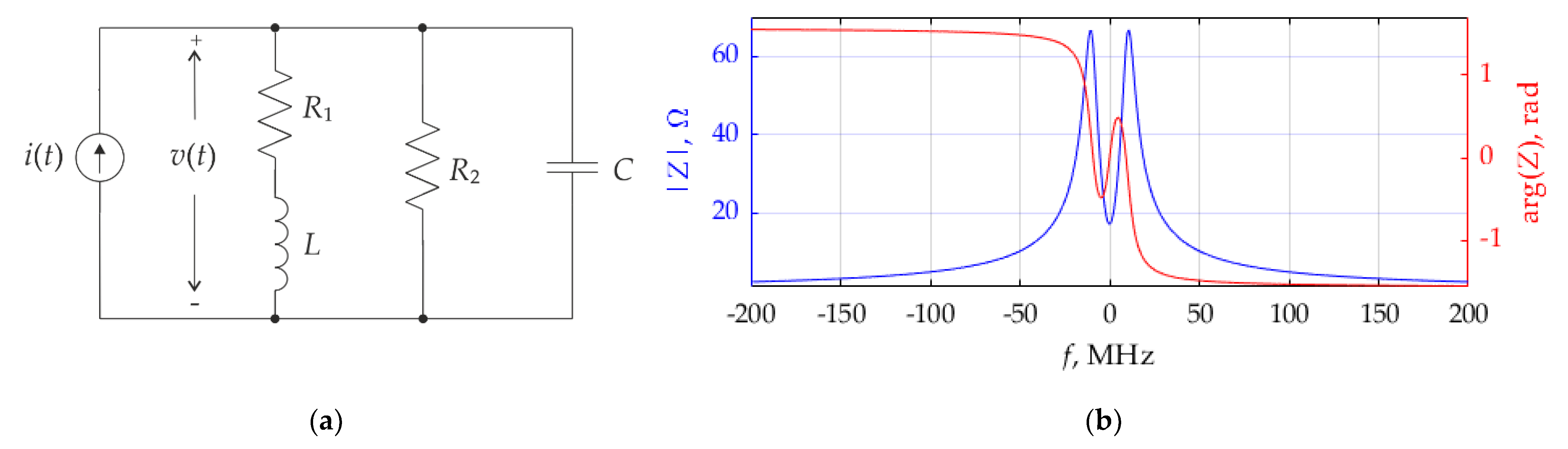
The parallel resonant circuit with feeding current source, which is presented in Figure 1a, was chosen for numerical simulation. The following parameters of the circuit were established: R₁ = 20 Ω, R₂ = 125 Ω, L = 0.8 mH, C = 320 nF. Those parameters make it possible to determine the following circuit characteristics: Q factor Q = 1.25, resonant frequency f_r = 10 MHz, characteristic impedance ρ = 50 Ω.

The FR describing the input impedance of the circuit is defined as:

$$Z(f)=\frac{R_1{R}_2+j2\pi fL{R}_2}{-4{\pi }^2{f}^{2}LC{R}_1{R}_2+j2\pi f(L+R_1{R}_{2}C)+R_1+R_2}.$$

(57)

The input impedance of the circuit versus frequency is presented in Figure 1b, where its absolute value and phase are combined in the same double sided plot.

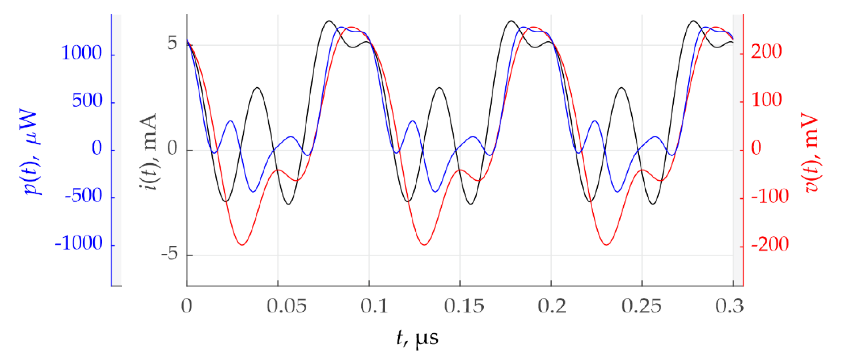
3.1. Finite Sum of Harmonics Current Excitation

The periodic current i(t), consisting of three sinusoids and a dc component with period T = 0.1 μs, is considered as the first example:

$$i(t)=2+3\cos \left(2\pi Ft+\frac{\pi }{4}\right)+2\cos \left(4\pi Ft+\frac{\pi }{2}\right)+2\cos \left(6\pi Ft-\frac{\pi }{3}\right)\left[\mathrm{mA}\right],$$

(58)

where the frequency is F = 1/T = 10 MHz.

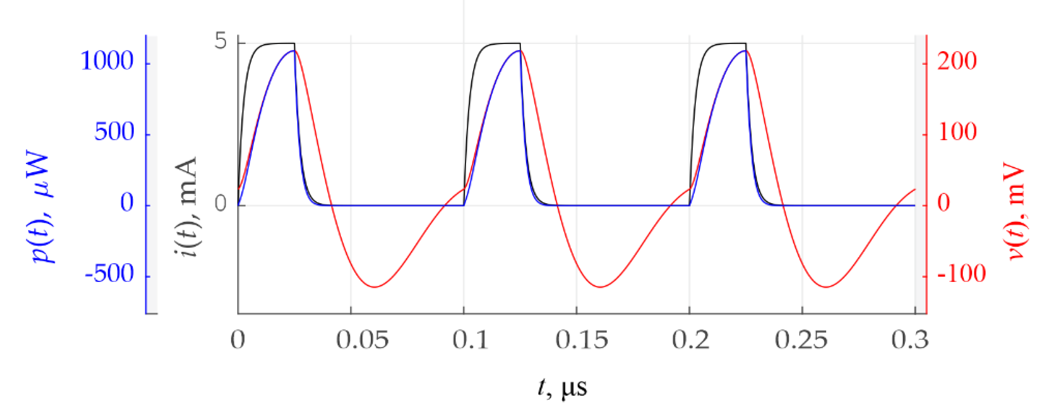
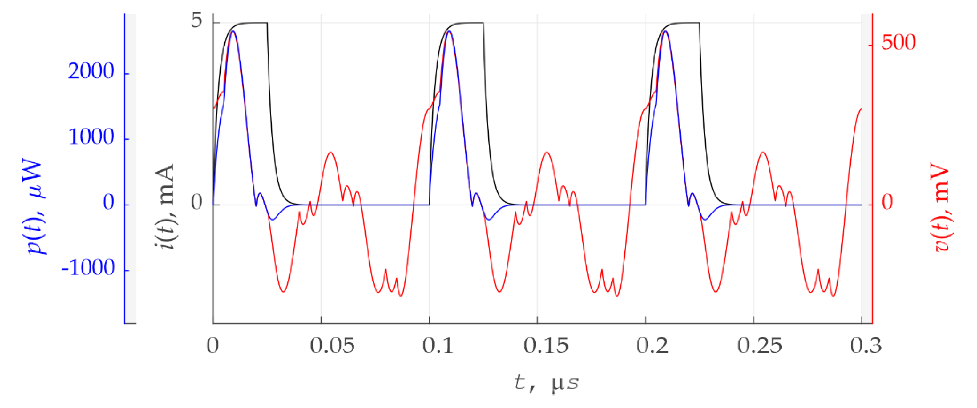
The current, i(t), voltage, v(t), and power, p(t), signals are depicted in Figure 2. They are periodic functions with the same period, T.

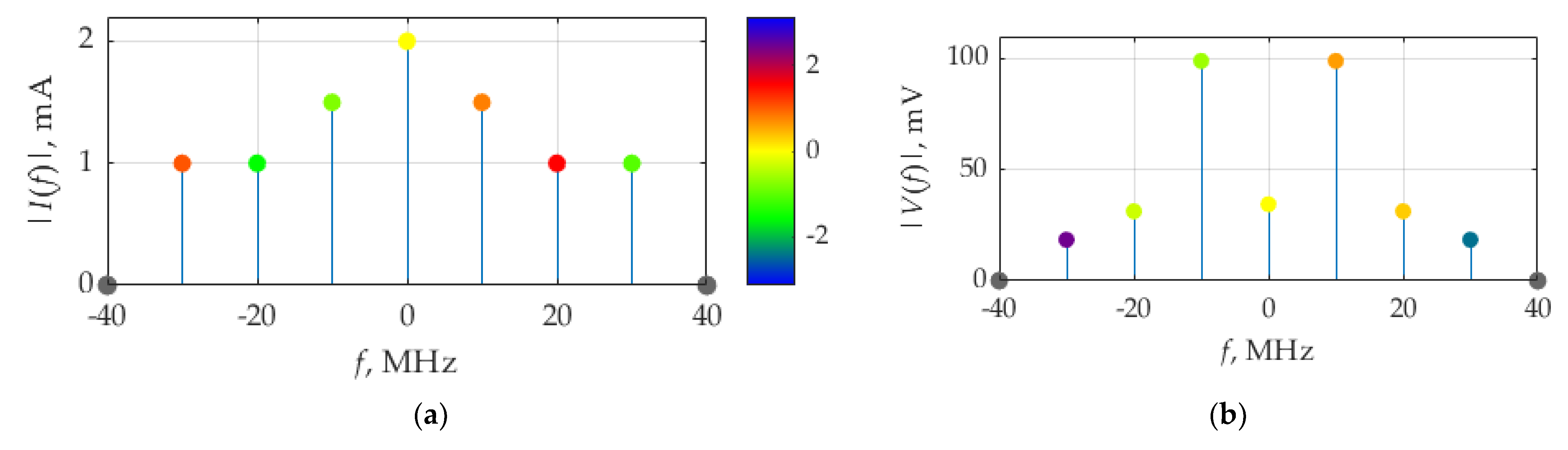
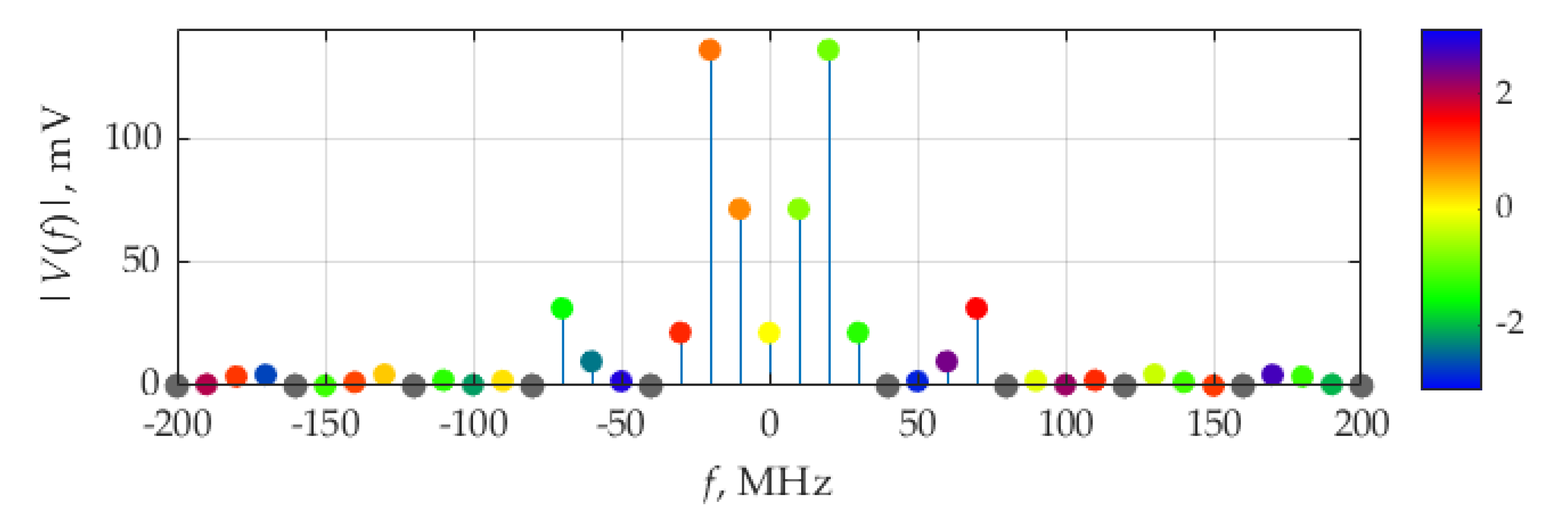
The spectra of current, i(t), and voltage, v(t), are presented in Figure 3a,b, respectively, as the weights of the Dirac delta functions representing Fourier coefficients (5) and measured in [A] and [V], respectively. The colors of the circles designate the phase of each Fourier coefficient, according to the color bar, ranging from −π to π. The same visualizing technique will be used for revealing the phase information in other figures.

It can be seen in Figure 3b that, for the voltage spectra, the maximum in absolute value weights of the delta function are at frequencies ±10 MHz, which correspond to the circuit resonant frequency, f_r, and the fundamental frequency, F, of considered signals.

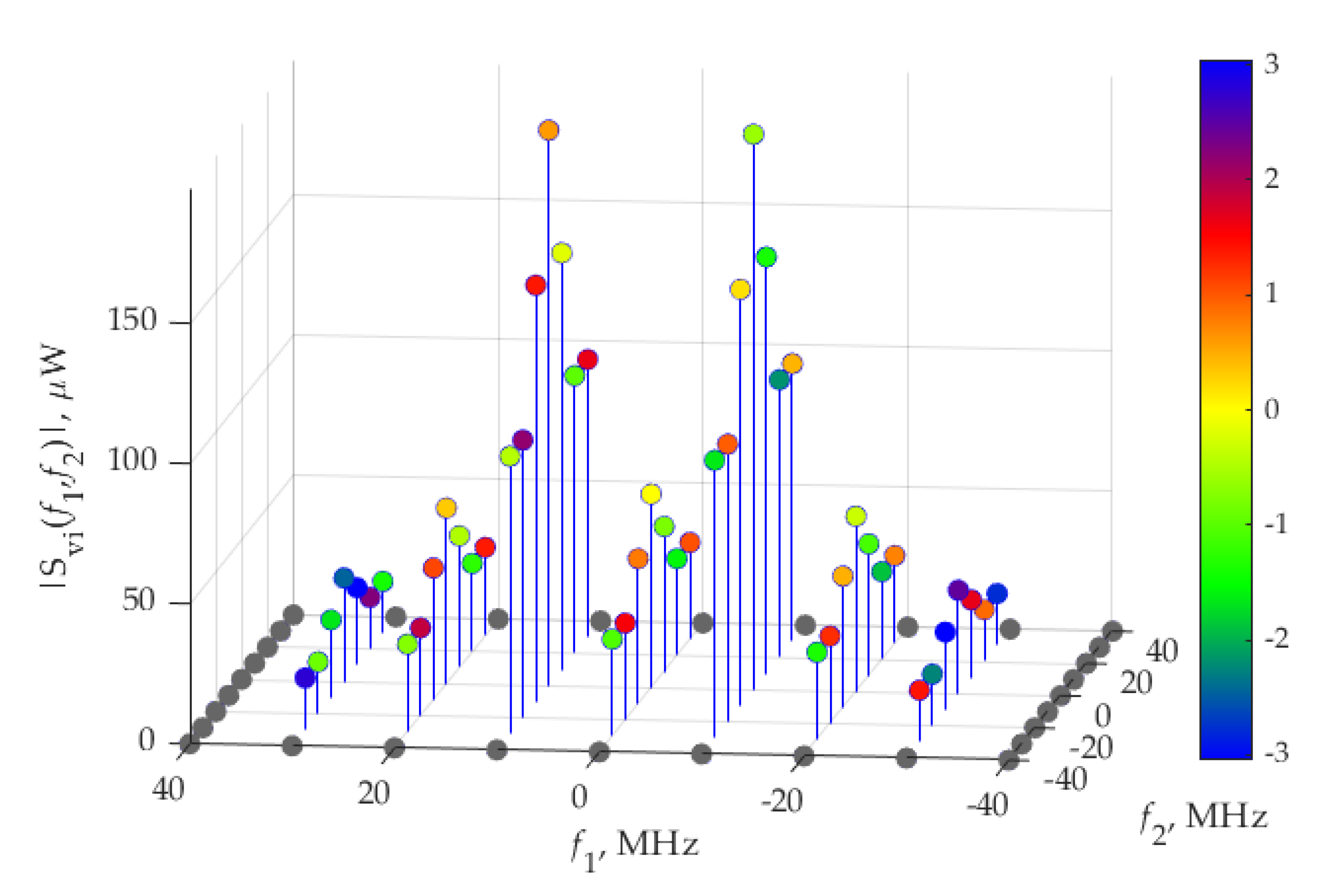
Figure 4 shows the weights of two-dimensional Dirac delta functions, forming the bifrequency spectrum, S_vi(f₁, f₂), of the current, i(t), and the voltage, v(t), in accordance with (15). These delta functions are arranged with step 10 MHz, which corresponds to the fundamental frequency, F, of signals i(t), v(t) and p(t). It can be seen that the section of S_vi(f₁, f₂) at f₁ = ±10 MHz have maximum weights.

The absolute values, in μW, and phases, in radians, of the delta function weights forming the bifrequency spectrum, S_vi(f₁, f₂), are presented in

Table 1. The amplitudes and phases of the bifrequency spectrum.

	Frequency f2, in MHz
Frequency f1, MHz		−30	−20	−10	0	10	20	30
	−30	18.5 ∠ 1.41	18.5 ∠ −2.26	27.7 ∠ −3.04	36.9 ∠ 2.45	27.7 ∠ 1.67	18.5 ∠ 0.88	18.5 ∠ −2.78
	−20	31.3 ∠ −1.36	31.3 ∠ 1.26	46.9 ∠ 0.47	62.8 ∠ −0.32	46.9 ∠ −1.10	31.3 ∠ −1.89	31.3 ∠ 0.73
	−10	99 ∠ −1.65	99 ∠ 0.97	148.5 ∠ 0.18	198 ∠ −0.6	148.5 ∠ −1.39	99 ∠ −2.17	99 ∠ 0.44
	0	34.5 ∠ −1.05	34.5 ∠ 1.57	51.7 ∠ 0.79	69 ∠ 0	51.7 ∠ −0.79	34.5 ∠ −1.57	34.5 ∠ 1.05
	10	99 ∠ −0.44	99 ∠ 2.17	148.5 ∠ 1.39	198 ∠ 0.6	148.5 ∠ −0.18	99 ∠ −0.97	99 ∠ 1.65
	20	31.3 ∠ −0.73	31.3 ∠ 1.89	46.9 ∠ 1.10	62.5 ∠ 0.32	46.9 ∠ −0.47	31.3 ∠ −1.26	31.3 ∠ 1.36
	30	18.5 ∠2.78	18.5 ∠ −0.88	27.7 ∠ −1.67	36.9 ∠ −2.45	27.7 ∠ 3.04	18.5 ∠ 2.26	18.5 ∠ −1.41

, where each cell corresponds to a pair of frequencies, f₁ and f₂, defined in the rows and columns, respectively.

The alternative representation of the bifrequency spectrum is the diagram shown in Figure 5a, where each delta-function is depicted as a circle whose area is proportional to the absolute value of S_vi(f₁, f₂). This way of presenting a 3D image of S_vi(f₁,f₂), on plane, can be convenient for the visualization and rapid estimation of the relative values of S_vi(f₁,f₂) components. We preferred to use a diagrammatic representation in subsequent typical cases. The frequencies f₁, f₂ range from −30 to 30 MHz.

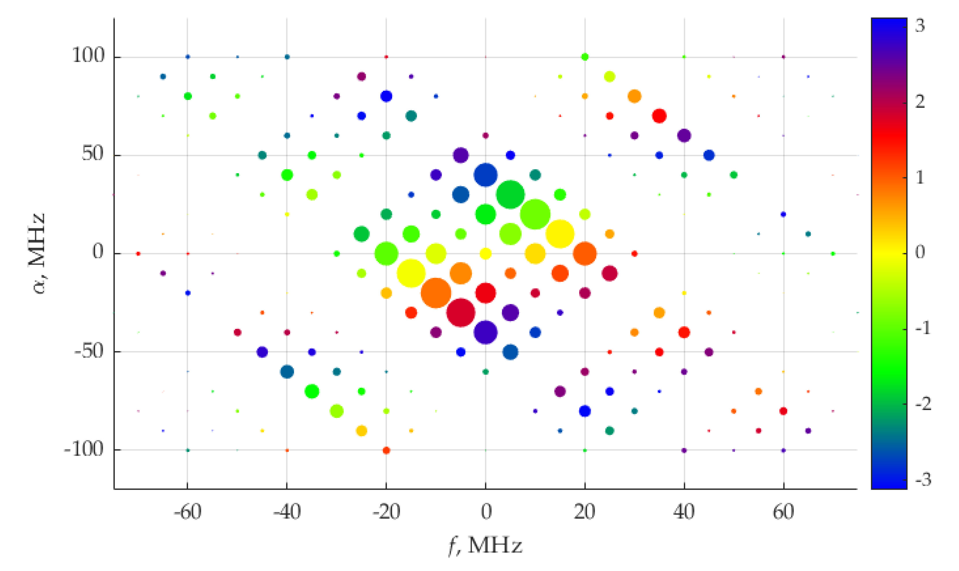
Figure 5b shows the diagram of CSCD S_vi(α,f) (21), where the weights (22) of delta functions are presented. The cyclic frequency, α, ranges from −60 to 60 MHz, the frequency, f, ranges from −30 to 30 MHz.

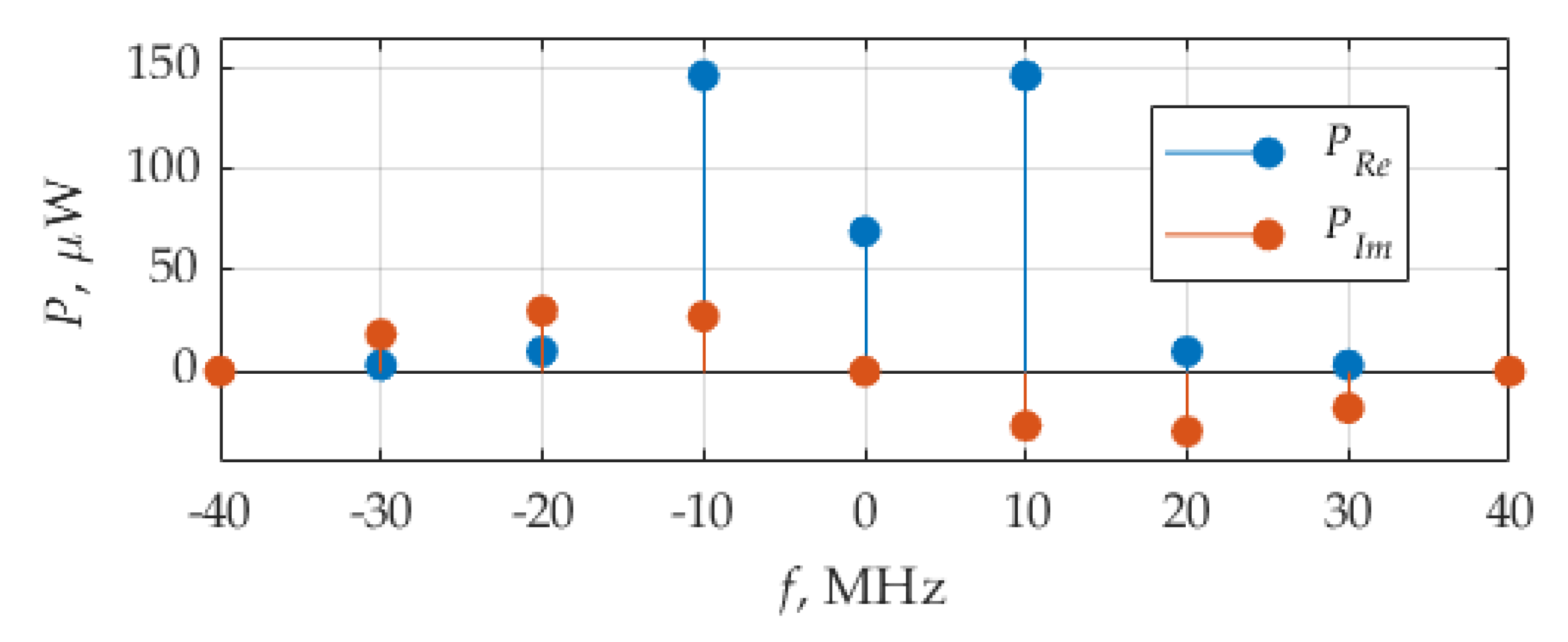
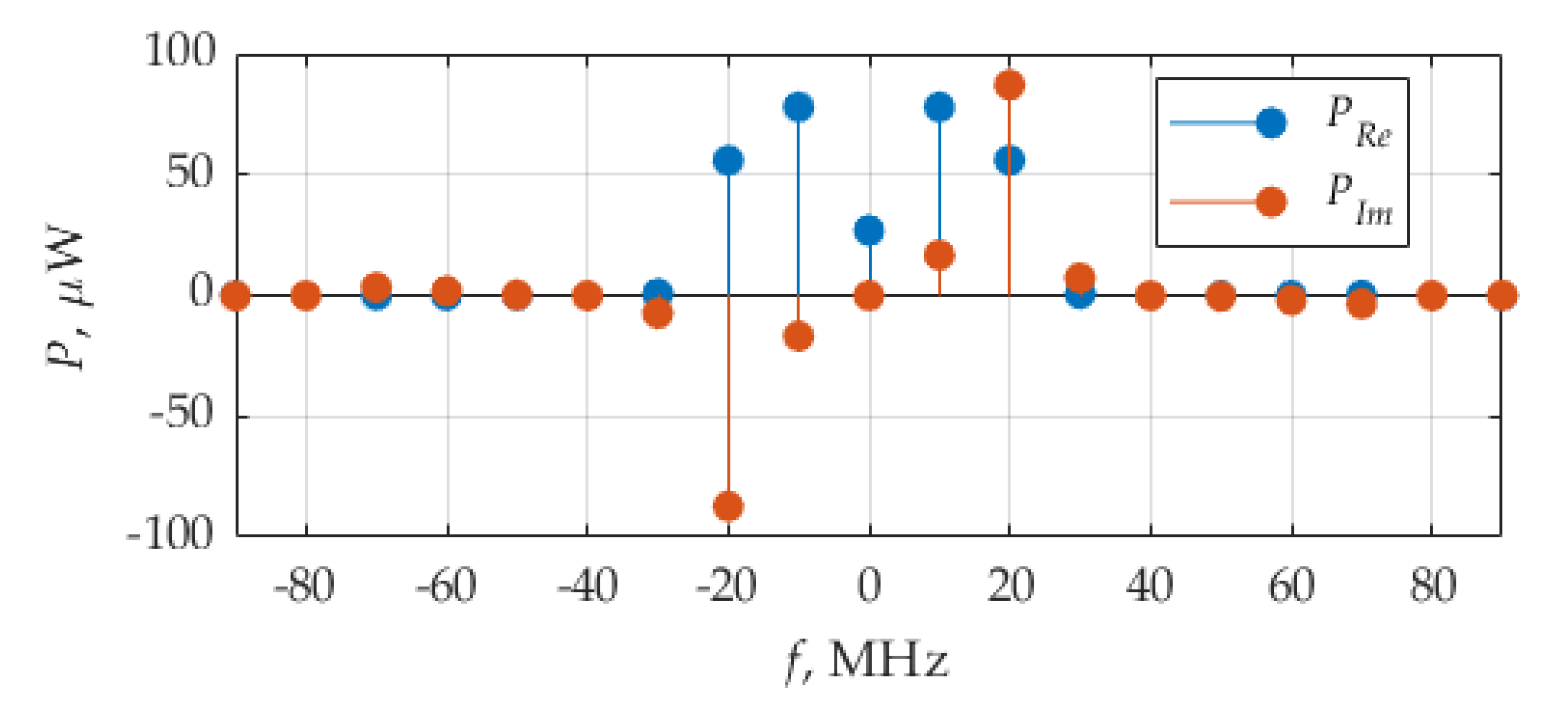
Figure 6 shows the distribution of the real and imaginary parts of average power. It can be seen that the real part contributes, in average power, more than the imaginary part. The weights of the delta function of the real part are highest at frequencies ±10 MHz, which is the circuit resonant frequency, f_r, and the fundamental frequency, F, of considered signals.

Figure 7 shows the spectrum of p(t). The delta functions forming the spectrum of instantaneous power p(t) are at the same frequencies as the delta functions forming the spectrum of instantaneous current i(t) and voltage v(t) because they are periodic functions with the same period.

The following quantitative power characteristics were calculated: the average power (33) P_av = 386.5 μW, apparent power (39) P_app = 541.2 μVA, power factor (43) PF = 0.71.

These power quantities can be verified using the traditional method. The periodic voltage v(t), which is depicted in Figure 1a, can be found analytically using frequency characteristic (57). Its formal representation, which is written with 2-digit precision for the sake of compactness, is as follows:

$$v(t)=34.5+198\cos \left(2\pi Ft+0.6\right)+62.6\cos \left(4\pi Ft+0.32\right)+36.9\cos \left(6\pi Ft-2.45\right)\left[\mathrm{mV}\right].$$

(59)

The effective values of the voltage V_eff and current I_eff, evaluated using (40) and (41), are, respectively, 153.0825 mV and 3.5355 mA, whose product yields the apparent power by definition (39): P_app = 541.2 μVA.

As soon as the voltage and current are known in closed form, the average power P_av can also be evaluated analytically using (32) where the substitution p(t) = v(t)i(t) is made and the integration limits are chosen from 0 to T = 1/F. This yields P_av = 386.5 μW, which is exactly the same value as found above.

3.2. Pulse Train Current Excitation

The second example of signal i(t) to consider is a periodic train of rectangular pulses followed with period T = 0.1 μs, with exponentially smoothed leading and trailing edges. The current i(t) can be defined as:

$$i(t)={\displaystyle \sum _{n=-\infty }^{+\infty }{i}_1(t-nT)}[\mathrm{A}],$$

(60)

where

$$i_1(t)=\left(u(t)-u(t-\Delta )\right)\left(1-e^{-\alpha t}\right)+u(t-\Delta )e^{-\alpha t}\left(e^{-\alpha \Delta }-1\right),$$

(61)

where u(t) is Heaviside function, and the time constant Δ = 1/α is equal to one tenth of the width of each pulse. The current, i(t), voltage, v(t), and power, p(t), signals are depicted in Figure 8. They are periodic functions with the same period, T.

The spectra of current i(t) and voltage v(t) are presented in Figure 9 and Figure 10, respectively. The spectrum (Figure 9) of the current (60) contains more harmonics” in comparison with the spectrum (Figure 3a) of the current (58), discussed above. However, the voltage spectra in Figure 3b and Figure 10 consist of a similar number of meaningful delta functions because the absolute values of delta functions related the components higher than the third become negligible. For the case of the voltage excited by the pulse current, this can be explained by the selective properties of resonant circuits. It can be seen in Figure 10 that delta functions having the maximum weights by absolute value are at frequencies ±10 MHz, which correspond to the circuit resonant frequency, f_r, and the fundamental frequency, F, of the considered signals.

Figure 11 shows the diagram of CSCD S_vi(α,f) found in accordance with (21). It has more components than the diagram in Figure 5b because of the richer spectral composition of the rectangular pulse train current (60).

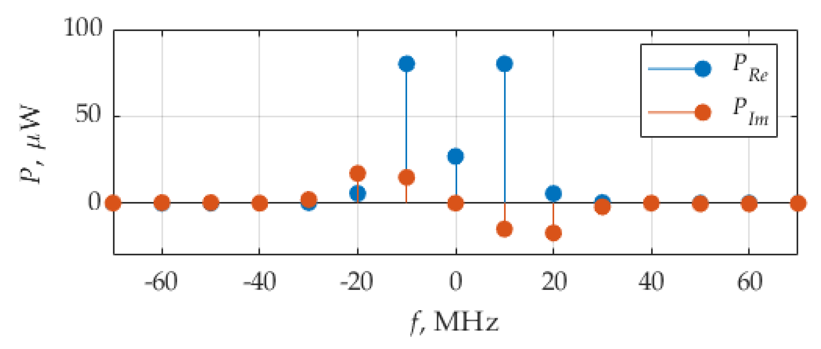
Figure 12 shows the distribution of the real and imaginary parts of average power. The weights of the delta function of the real part are maximum at frequencies ±10 MHz, which match the circuit resonant of the fundamental frequencies of the signal under investigation.

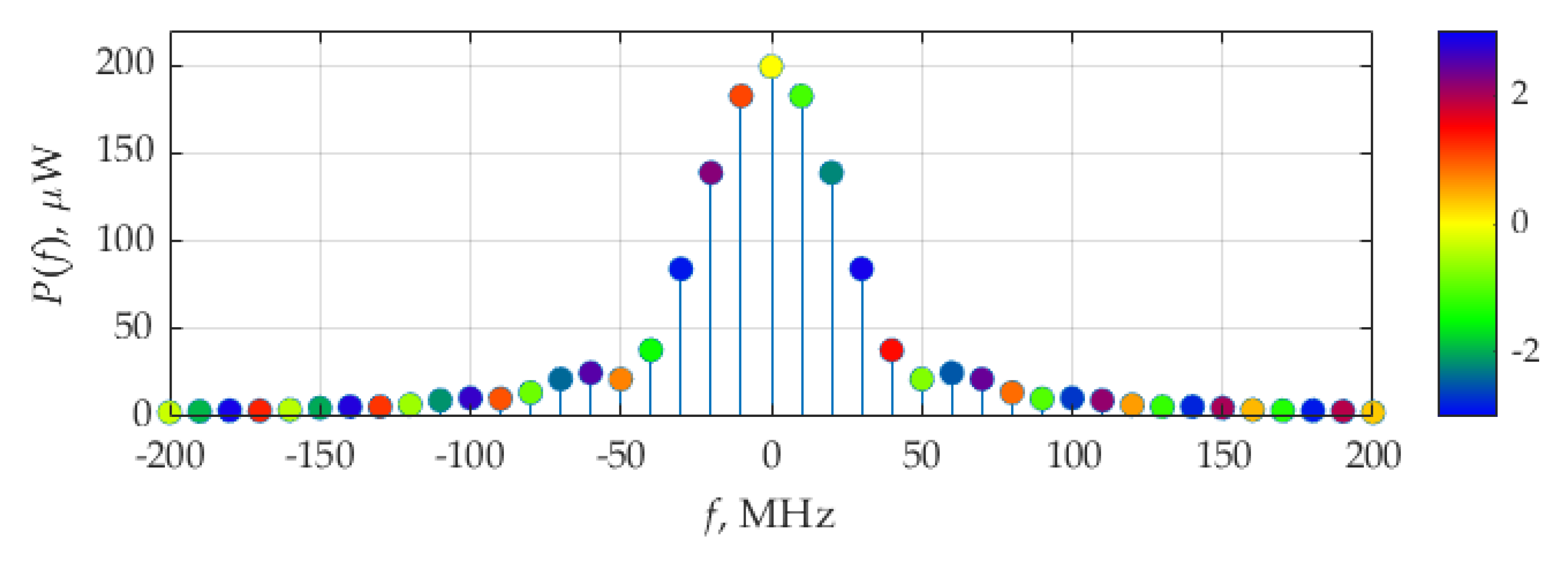
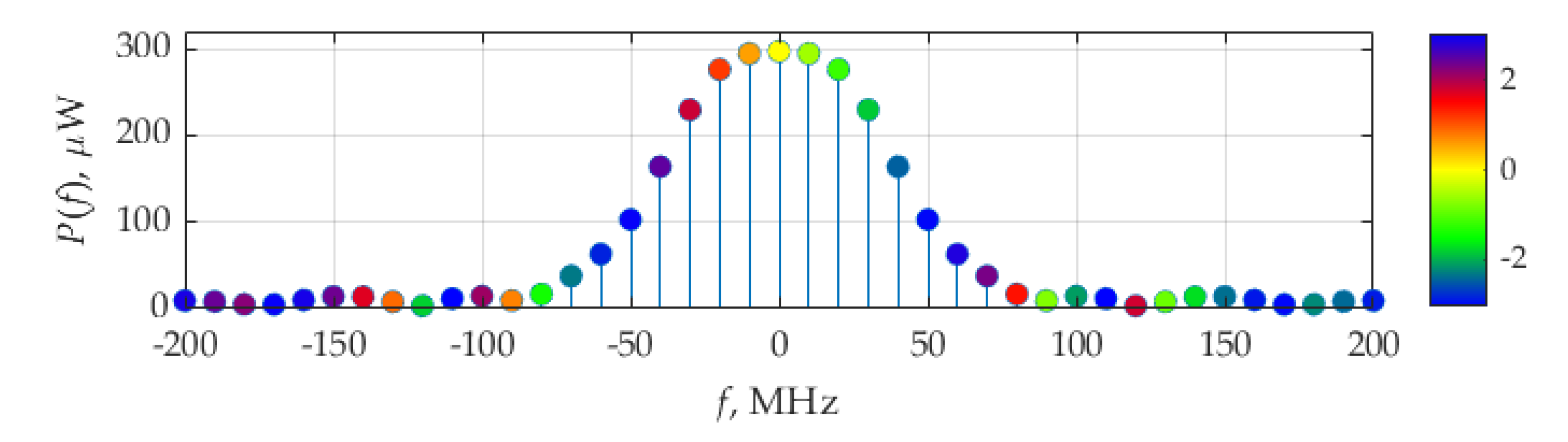
Figure 13 shows the spectrum of instantaneous power p(t). The delta functions forming the spectrum of p(t) are at the same frequencies as the delta functions forming the spectrum of instantaneous current, i(t), and voltage, v(t), signals.

The following quantitative power characteristics were calculated: the average power (33) P_av = 199.4 μW, apparent power (39) P_app = 264.7 μVA, power factor (43) PF = 0.75.

3.3. Trasmission Line Example

The third example is a lossless transmission line (Figure 14a) with a load, which coincides with the load of the circuit in Figure 1a.

The input impedance of transmission line can be evaluated as [48]:

$$Z_{in}(f)=\frac{Z(f)\cos \left(\frac{2\pi fl}{c}\right)+j{Z}_0\sin \left(\frac{2\pi fl}{c}\right)}{\cos \left(\frac{2\pi fl}{c}\right)+j\frac{Z(f)}{Z_0}\sin \left(\frac{2\pi fl}{c}\right)},$$

(62)

where c is the speed of wave propagation, l is the length of transmission line, Z is defined by the formula (1), and Z₀ is characteristic impedance. For numerical simulation, the following parameters were chosen: c = 3 × 10⁸ m/s, Z₀ = 50 Ω, l = 12 m.

Consider the current source, which is the same as in the second example, defined by formulas (60) and (61). The input impedance versus frequency is presented in Figure 14b, where its absolute value and phase are combined in the same double sided plot.

The current, i(t), voltage, v(t), and power, p(t), signals are depicted in Figure 15. They are periodic functions with period T.

The spectrum of current i(t) is the same as in Figure 9, the spectrum of voltage v(t) is presented in Figure 16. It can be seen that the maximum by absolute weight value delta function are at frequencies ±20 MHz. This can be explained by the higher absolute value of the input impedance (62) at frequencies ±20 MHz, compared to ±10 MHz.

Figure 17 shows the diagram of CSCD S_vi(α,f) (21). It has even more components than diagram in Figure 11 because more spectral components of |V(f)| in Figure 16 have sufficient value, compared to |V(f)| in Figure 10.

Figure 18 shows the distribution of the real and imaginary parts of average power. The weights of the delta function of the real part are maximum at frequencies ±10 MHz, which correspond to fundamental frequency, F, of the considered signals. The imaginary part of delta function weights is maximum by its absolute value at frequencies ±30 MHz.

Figure 19 shows the spectrum of p(t). The delta functions forming the spectrum of instantaneous power p(t) are at the same frequencies as the delta functions forming the spectrum of instantaneous current i(t) and voltage v(t). The first five spectral components are higher with respect to the dc component than took place in the case of the resonant circuit without transmission line (Figure 13).

The following quantitative power characteristics were calculated: the average power (33) P_av = 297.1 μW, apparent power (39) P_app = 537.2 μVA, power factor (43) PF = 0.55.

4. Discussion on Conservation Law

From its definition (18), CCF suggests performing the multiplication of time shifted versions of the voltage and current. We are going to show, in this section, that this can lead us to important properties linking the components of CSCD (22) over all the elements of which any circuit consists.

Let us consider an electric circuit assembled of N elements, whose currents and voltages are denoted by i_n(t) and v_n(t), respectively. Tellegen’s theorem [10] states that, whenever the currents obey the equation set constituting Kirchhoff’s current law and the voltages obey the equation set constituting Kirchhoff’s voltage law (KVL), the instantaneous powers p_n(t) = v_n(t)i_n(t) will submit to the balance equation:

$${\displaystyle \sum _{n=1}^N{p}_n(t)}={\displaystyle \sum _{n=1}^N{v}_n(t)i_n(t)}=0.$$

(63)

The equation expressing KVL in the lth loop looks like the linear combination of the voltages:

$${\displaystyle \sum _{n=1}^N{\lambda }_{ln}{v}_n(t)}=0,$$

(64)

where λ_ln is a coefficient taking one of three possible values: 1, −1 or 0. If the element has not been included in the lth loop, λ_ln = 0. If the nth element is a part of the loop, the mutual directions of the element voltage and the loop trace determine λ_ln = 1 if they coincide, and λ_ln = −1 otherwise. The structure of equation set describing KVL establishes the fact that they are invariant to time shift θ applied to all voltages, v_n(t + θ), simultaneously.

Similarly, the equation for KCL in the pth node is the linear combination of the currents:

$${\displaystyle \sum _{n=1}^N{\beta }_{pn}{i}_n(t)}=0,$$

(65)

where β_pn is a coefficient taking values out of the set {1, −1, 0}. If the nth element is not adjacent to the pth loop, β_pn = 0. If the current associated with the nth element is leaving the node, β_pn = 1, and if the current is entering the node, β_pn = −1. Provided the time shift σ applied to all currents, i_n(t + σ), simultaneously, the KCL equation set remains valid.

More importantly, time shifts applied to voltages and currents do not need to be equal to each other. Returning to the genuine Tellegen’s theorem, we may conclude that:

$$\forall (t,\tau )\in {ℝ}^2:{\displaystyle \sum _{n=1}^N{\mathcal{R}}_{vin}(t,\tau )}={\displaystyle \sum _{n=1}^N{v}_n(t+\tau /2)i_n^{\ast }(t-\tau /2)}=0,$$

(66)

where the additional index, n, written in the subscript of ${\mathcal{R}}_{vin}(t,\tau )$, highlights the possession of CCF by the nth element of the circuit. Equation (66) provides us with a generalized version of Tellegen’s theorem in a time domain.

However, the series made of Dirac delta functions in (21) forms the frequency domain counterpart of orthogonal basis for formal expansion of CCF into double Fourier series:

$${\mathcal{R}}_{vi}(t,\tau )={\displaystyle \sum _{m=-\infty }^{+\infty }{\displaystyle \sum _{k=-\infty }^{+\infty }{\mathcal{S}}_{vi}^{(m,k)}\exp \left\{j2\pi \left[mFt+\left(k+\frac{{((m))}_2}{2}\right)F\tau \right]\right\}}}.$$

(67)

In other words, provided the complex exponential term is rewritten into a concise expression:

$$E_{m,k}(t,\tau )=\exp \left\{j2\pi \left[mFt+\left(k+\frac{{((m))}_2}{2}\right)F\tau \right]\right\},$$

(68)

the orthogonality condition will hold:

$$\frac{1}{2T^2}{\displaystyle \underset{T}{\int }{\displaystyle \underset{2T}{\int }{E}_{m_1,k_1}(t,\tau )}}{E}_{m_2,k_2}^{*}(t,\tau )d\tau dt={\delta }_{k_1{k}_2}{\delta }_{m_1{m}_2},$$

(69)

where δ_pq denotes the Kronecker delta, which is equal to 1 if p = q and 0 otherwise.

Having applied the component wise orthogonality property to relation (66), we come to a new version of the conservation law:

$$\forall (m,k)\in {\mathbb{Z}}^2:{\displaystyle \sum _{n=1}^N{\mathcal{S}}_{vin}^{(m,k)}}=0,$$

(70)

which means that each component of (22) obeys the conservation law separately.

The direct yet useful corollary of conservation law (70) is the fact that an appropriately chosen function, depending on a subset containing some of the components, will also submit to the conservation law. In particular, a sum of individually transformed components can assemble a function of such a type:

$${\displaystyle \sum _{n=1}^N{y}_n}=0,\hspace{1em}{y}_n={\displaystyle \sum _{(m,k)\in \mathcal{V}}g\left({\mathcal{S}}_{vin}^{(m,k)}\right)},$$

(71)

where g() defines a one variable function, satisfying a linearity condition, and $\mathcal{V}\subset {\mathbb{Z}}^2$ determines the set of pairs (m, k) chosen for performing the summation.

For instance, the average power (33) and the coefficients of Fourier series (31), which is expressing the instantaneous power, can be treated this way if the function g(x) = x and $\mathcal{V}=\left\{M\right\}\times \mathbb{Z}$, where scalar M is the coefficient number: it will be equal to zero for the average power. Another example is combination:

$$Q_n=2{\displaystyle \sum _{k=1}^{+\infty }\Im \mathfrak{m}{\mathcal{S}}_{vin}^{(0,k)}},$$

(72)

which can be fairly treated as the reactive power, according to Budeanu’s theory [15]. It also obeys to the conservation law, as it follows from (70), with $g(x)=\Im \mathfrak{m}(x)$ and $\mathcal{V}=\left\{0\right\}\times \mathbb{N}$. On the other hand, some other transformations may not agree with componentwise equation (70). Thus, it should not be surprising that the apparent power (42), which actually does not obey the conservation law, as it has not got any reasons, rooted in (70), to be governed by it.

5. Conclusions

The approach proposed in this paper to power analysis in electric circuits under arbitrary periodic excitation suggests a systematic framework, which is mainly based on two ideas. The first is expressing the voltage across, and current through, an element by their complex valued Fourier series; this allows one to consider them as first order CS processes. The second idea consists in applying the set of conventional CS tools, such as CCF and SCF, to the voltage–current pair in the element under analysis.

The main advantages of the proposed method are generally based on its methodology. The method reveals the elementary, so called “atomic”, power components, which still obey the conservation law. Proper combinations of these components, including nonlinear, as for apparent power by (42), can be used for representing any quantity, characterizing power. As it is shown in this paper, the description based on CS properties perfectly matches the nature of instantaneous power as a product of the voltage and current related to the same element of electric circuit, or one port.

On the one hand, such an approach may look overly complicated since there exist alternative approaches to the same problem based on real valued, or amplitude and phase representation. The introduction of complex numbers for describing power components may be looking excessive, since complex Fourier series are more common for researchers dealing with signal processing tasks than for researchers working in the fields of electric machines and power delivery.

At the current development stage, the proposed method was implemented as a specialized software utility used for postprocessing the data obtained as the output of an applied software performing circuit analysis in steady state mode. One of the classes of the problems typically solved by means of this software is the numerical optimization of the power factor, which is to be achieved by the allowed variation of the load, e.g., by adding extra reactance or changing the length of the transmission line. However, the classical optimization approach is usually performed for a single harmonic, whereas the other harmonics are considered primarily as the distortion. In contrast, the proposed method utilizes the compact component wise representation of the full instantaneous power in the element of the circuit excited by an arbitrary periodic waveform. This paves the way to more accurate optimization procedures, taking into account higher harmonics of the signal.

Although, from an applied mathematician’s point of view, CCF can be treated as an extended model of the time varying instantaneous power, in which the auxiliary lag parameter has been introduced, the physical meaning of CCF may still require deeper clarification. Thus, although each of the components given by (22) obeys conservation law (70) separately, they will contribute to the Fourier series representing the instantaneous power (30) only in aggregated form (31). Other aggregations are carried out to form the average and reactive powers. In addition, the question of the realizability of the circuit, which can implement the product of the time-translated voltage and currents, is omitted in this paper, leaving this issue open.

Future development of the CS framework proposed in this paper can be carried out in several directions. The first one consists in its application to the circuits containing nonlinear or time varying elements. As soon as the simplified model of a nonlinear element is involved, the relation between the voltage and current in such an element can be described by its volt–ampere characteristics. In contrast, the time varying behavior of an element can be described by linear periodically time-varying, which are perfectly covered by the CS theory. In both cases, instantaneous power still remains periodic and keeps its representative ability as the quantitative measure of the voltage–current interaction.

Another generalization of the proposed theory can be performed if the circuit is excited by voltages and currents whose sources are modeled as random processes. Moreover, promising results are expected for cases of wide sense stationary and wide sense cyclostationary random processes. However, since the voltage and current cease to be deterministic, the expectation starts taking on an important part in the power representation. Not only can this procedure be carried out in a probabilistic manner using ensemble averaging, but it can also be performed in the infinite time limiting process, according to the concepts developed within fraction of time theory [49]. Those may also become the promising topics for further research.

Finally, after proper generalization, the proposed approach can be used for describing the power in a multiport, where voltages and currents can be measured in dedicated ports rather than separate elements. Furthermore, starting from voltage–current interaction, the approach may be used in electromagnetics for describing power produced by appropriate cross product electric and magnetic fields expressed as component vectors in three dimensional space.