Abstract
This paper presents the application of three non-destructive techniques in the study of an agricultural area on the west coast of Peloponnese, Greece. The applied methods include (a) electromagnetic geophysical research using a handheld EM profiler (EMP-400 GSSI), (b) computed tomography (CT) with coring data, and (c) X-ray Fluorescence (XRF) scanning. As electrical conductivity is mainly influenced by the bulk soil, including water content, clay content and mineralogy, organic matter, and bulk density, a comparison of the three applied techniques indicates the same soil stratification and same soil properties with depth. Moreover, the ground-truthing by the undisturbed soil and sediments core retrieved in the centre of the site as well as the laboratory analyses of soil and sediment properties confirm the reliability of the geophysical research and the revealed soil/sediment stratification.
1. Introduction
Non-destructive analytical techniques for soil and sediment investigation have undergone rapid development and can provide fast, low-cost, and continuous information compared to classical destructive methods [1,2]. By studying either soil properties or sediment cores, a much higher resolution can be achieved concerning geochemistry, textural features etc. Physical and chemical properties can be studied down to nanometre resolution, marking changes even on a seasonal scale. Furthermore, highlighting significant sections on sediment cores can lead to more targeted sampling.
In particular, X-ray-based systems, such as X-ray Fluorescence scanning and Computed Tomography scanning, have been established in the last decades as standard and common techniques. Both methods are based on the study of the wavelength that is produced by the incident of X-rays on a studied sample and the excitation of electrons that produces a movement from outer to inner shells. Later, characterization of the wavelength spectra to either specific elements or relative density can derive automatically through software. Therefore, recent studies, aim for better quantification of the prior mentioned systems, such as quantitative calibration of elemental intensities [3], internal sediment structure [4], porosity, microfauna internal and external structures [5], bioturbation [6], ichnofacies, and microfacies [7] in sediment cores as well as varve sediments structure [8,9].
In parallel to this field of detailed soil imaging, rapid advances are being made in various geophysical techniques for inferring the spatio-temporal variation of physical properties of the earth. These techniques are applied at various scales to obtain information on the underground structure, although at a much lower resolution than that achieved through CT and XRF scanning. However, geophysical prospecting provides an alternative means to examine soil structure at the scale of the outcrop and are easily extendable to larger scales in space and time. Thus, it is essential to test the synergetic potential of more traditional soil imaging techniques with geophysical methodologies and to assess their complementarity in studying wide areas (e.g., [10] and references therein).
Soil/sediments exploration by electromagnetic induction (EMI) is currently a widely accepted technique in precision agriculture, geological survey, and geophysics. The main advantages of the method are that (a) it is a non-invasive one, (b) it is fast and cost-effective, and (c) all the measurements can be easily geo-referenced [11,12]. Several studies correlate electrical conductivity (EC) with soil properties, such as percentage of clay fraction [13,14,15], water content [16], salt content [17], and organic matter [18]. The observed variations in soil electrical conductivity mainly depend on these soil properties. In agriculture, that can potentially influence crop growth and development [19]. For the in situ measurement of EC, several types of equipment are available. In the present study, we use GSSI EMP-400 of GSSI.
In this study, we present the results of a comparative application of CT, XRF, and Electro-Magnetic geophysical measurements in the area of the former marsh field Agoulinitsa, currently agricultural fields, which is located in western Peloponnese, Greece (Figure 1). The first overview of XRF data and CT scanning has already been discussed [20], so in this study, we primarily focus on the results of all three methods, highlighting their synergetic and complementary character toward studying soil characteristics of the studied area.
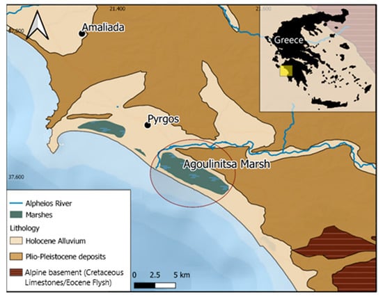
Figure 1.
Geological map of the study area, with Agoulinitsa marsh field, highlighted in red circle. The site location is marked in yellow square at the overview map of Greece on the top right corner.
2. Study Area
The western coast of Peloponnese (Figure 1) is characterized by an array of barrier accretion plains, coastal dune fields, and deltas along with barrier lagoons and peripheral marshes [21]. The area is fed by significant rivers such as Alpheios as well as smaller streams and is influenced by marine depositional processes in the littoral zone. Thus, dynamic coastal environments are prone to climatic, sea level, tectonic, and human-induced changes. Therefore, previous studies in Peloponnese focused on palaeoenvironmental [21,22,23] and palaeoclimatic reconstructions [24,25,26], changes in sedimentation [27,28,29], sea-level changes [30], and high-energy events [31,32,33,34], many of which were in archaeological contexts.
Agoulinitsa marsh is located at the Kyparissia Gulf, south of the Alpheios river mouth (Figure 1). Formerly Agoulinitsa marsh, it was drained artificially in 1969 and used for agriculture from then on. The area consists of white to light brown limestones overlain by Plio-Pleistocene marine sandstones, sandy clays, and marls [35,36] (Figure 1). The lowlands consist of Holocene alluvial deposits made up of colluvium, fluvial sediments, coastal dunes, and beach deposits [37] (Figure 1). Past and present high tectonic activity, accounting for one of the highest in Greece [38], which is attributed to the proximity to the outer part of the Hellenic arc convergent boundary, further triggered diapiric phenomena [39].
3. Material and Methods
3.1. Coring and Sedimentological Analysis
The soil/sediment core for the ground-truthing stratification, CT and XRF scanning, was extracted from the Agoulinitsa marsh using an Eijelkamp vibrating corer, with stainless steel tubes and plastic liners (1 m length, 5 cm diameter), ensuring undisturbed and uncontaminated soil/sediments sampling. After its extraction, the 4 m long core was sealed with cling film to preserve its moisture and moved to the Laboratory of Sedimentology of the University of Patras for further analysis.
In addition to the detailed imaging analysis, described in the following section, sedimentological analysis was performed on 30 samples from the Agoulinitsa core. This included grain size analysis and total organic carbon (TOC) measurements. For the grain size analysis, a Malvern Mastersizer, Hydro 2000 was used and the samples were classified based on [40] nomenclature. Total organic carbon content (TOC) was determined according to the titration method of [41,42,43].
3.2. CT Scanning
The CT scan analysis of the Agoulinitsa soil core was conducted at the University Hospital of Patras, using a Toshiba Aquilion Prime CT scanner. The core was studied in sections of 1 m length, and the acquisition parameterization was optimized to achieve the finest possible resolution. More specifically, we adopted a slice thickness of 0.5 mm, a slice interval of 0.3 mm, a helical rotation with a pitch factor of 0.637, tube voltage of 120 kV, and current of 350 mA. For the CT images, the calculated value was expressed in HUs (Hounsfield units), where HU = ((μmatter − μwater)/μwater) × 1000, with μ representing the linear attenuation coefficient. Medical CT scanners were set with default HU values of −1000 for air and 0 for water.
The 2D HU value profile of the sediment core was acquired through the MatlabTM based software SedCT [44]. The software was composed of the main interface (SedCT) and an add-on (SedCTimage). In the main interface, the DICOM files from each core section were inserted, and after adjusting the parameters, in response to the study core, the downcore profile of the mean HU value was presented. In our application, every 1 m of the core was represented by 3400 DICOM files. Upon completing the first step, the exported files were inserted into the secondary interface (SedCT image), where a chromatic or greyscale 2D model was produced.
The 3D model of the studied core was constructed through the medical software Inobitec (Russian Federation). After inserting the DICOM files for each core section, we facilitated the Multiplanar reconstruction (MPR) in order to have a complete overview of the core. The next step was the construction of the model, which was achieved through volume reconstruction. Since the software has been developed and used for medical purposes, alterations were needed in its parameterization in order to achieve the best visual result, meeting the needs of the samples and scale examined herein.
3.3. XRF Scanning
Semi-quantitative elemental concentrations were measured for the 4 m sediment core by an Avaatech X-ray Fluorescence core scanner at the Institute of Geosciences at Kiel University. The resolution was set at 0.5 cm, and the scanning was performed with a Molybdenum tube, set at 10 kV and 30 kV, with an integration time of 60 s per measurement. To avoid closed-sum effects, all measured intensities were presented as log10 ratios [1,45].
3.4. Electromagnetic Survey—EM Profiler
EM profiles in the field of Agoulinitsa were acquired using a multi-frequency EM conductivity meter, the EMP-400 Profiler of the Geophysical Survey Systems Incorporation (GSSI). The instrument is portable, carries both the transmitting and receiving coils required to measure the EM field, and does not require direct contact with the ground while measuring. This facilitated data collection, allowing for fast implementation of several measuring profiles above the study field. Subsequently, profile conductivity measurements were combined using appropriate software to create subsurface conductivity maps, which in turn, provide information on subsurface deposits, porosity, and soil properties and structures.
The study area (4.5 hectares) was covered by a set of line measurements (profiles) of 400 m in length and with a spacing of 10–12 m (Figure 2). This griding resulted in 9 profiles, named emTST01-09, which are plotted in Figure 2, along with the location of the sample core (marked in Figure 2 as “Core AG”). For each profile, EMP-400 was set to automatically take measurements every 0.5 s, while the operator was walking at a steady pace. Since EMP-400 is a multi-frequency measuring unit, we parameterized it to measure three distinct frequencies (1, 9, and 16 kHz) simultaneously to obtain information corresponding to shallow and deeper subsurface layers.
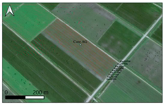
Figure 2.
Studied area with the location of the nine profiles scanned with the EMP-400 profiler and the location of core AG (4 m total length).
The subsequent step in our analysis comprised the 2D inversion of the collected data for the “quadrature” component of the EM signal, linked to conductivity. The inversion was performed using the EM4Soil-MF software package (EMTOMO, 2018), which was developed for data of multi-frequency instruments, such as the EMP-400 used in this study. The underlying inversion algorithm is the nonlinear, smoothness-constrained sort, proposed by [46]. A detailed description of the inversion algorithm is provided in the adopted software’s manual (EMTOMO, 2018).
4. Results and Discussion
4.1. Core Description
The sediment core was sub-divided into three sedimentological units, each one with specific textural and geochemical characteristics. Since the XRF core scanner provides a semi-quantitative geochemical profile, elemental concentrations are presented in log10 (base 10) ratios that can be interpreted in response to the environmental status of the marsh field.
The upper unit is characterized by the lowest HU values, therefore the lower relative density (Figure 3). The soil horizon is visible from 0.00 to 0.50 m, with unconsolidated organic-rich sediment. A significant differentiation of HU values before and after 0.50 m can be attributed to the water content of the sediment. From 0.00 to 0.50 m, the unconsolidated soil horizon is primarily composed of organic residues and shell fragments, visible in the CT scan section. Water content is significantly lower, compared with the water clogged section from 0.50 to 1.00 m. Increased organic content in this unit is also marked by the increased values of the Br/Cl ratio [47].
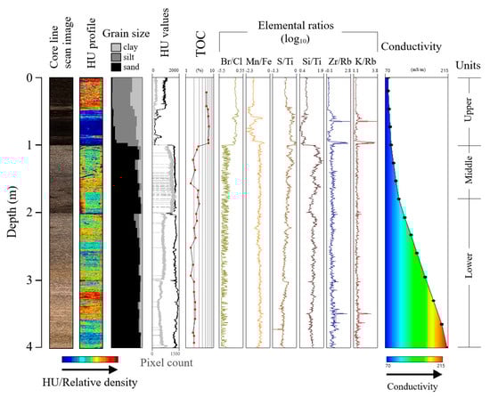
Figure 3.
Log profile of core AG presenting a line scan image of the core, 2D HU profile, grain size analysis, HU absolute values, Total Organic Carbon (TOC), elemental ratios in log10 scale, and mean conductivity as measured by the EMP-400 profiler.
The middle unit is characterized by a distinct transition to coarser material. HU presents higher values due to the increased relative density and the decreased water content compared with the upper section. Organic matter and root remains are visible on the CT scan sections. The Br/Cl ratio declines, and this trend is in accordance with the lower values of organic content (TOC). An increase in Si/Ti is associated with the sand fraction [48] in this unit and presents a monotonous signal. Mn/Fe also increases in this section, indicating more toxic conditions [49,50].
The lower unit presents a monotonous distribution of all studied parameters with no distinct variations. HU presents similar values to the prior unit due to the sediment’s similar characteristics. However, no root remnants or organic residues were identified throughout the lower unit.
Grain size values (sand, silt, and clay) and the TOC content measurements are also presented in Table S1 (Supplementary Materials).
4.2. Non-Destructive Techniques
Figure 4 also includes the derived variation of soil electrical conductivity with depth at the coring site. Multiple vertical profiles have been extracted from the geophysical line passing above the coring site (emTST06, Figure 2), within +/−2.5 m surface distance from it, and all show a gradual increase in the measured quantity with depth, which ranges from circa 70 mS/m close to the ground surface to 215 mS/m at the depth of 4 m. The linear increase in conductivity with depth is very slow within the top 1 m (almost constant, if considering spatial variability), slightly accelerates between 1–2 m, and shows a clear change in rate at the depth of 2 m. These depths of conductivity rate changes are in excellent agreement with the boundaries determined and described earlier based on the core analysis. Although the increasing trend of conductivity with depth contradicts the density distribution of materials in the soil profile, it may be explained by the increase in water content with depth and its elevated salinity due to the proximity of the site to the seashore.
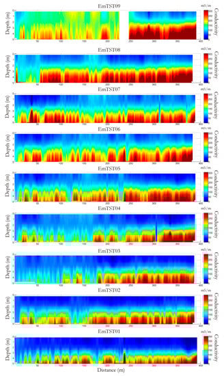
Figure 4.
Electrical conductivity profiles as extracted by the EMP-400 profiler from the studied field.
The consistency between core analysis results and geophysical measurements concerning the identification of sections in the soil/sediments stratigraphy is better pronounced when all measured profiles are examined. Figure 5 shows the inverted 2D distribution of conductivity along all nine profiles. Conductivity values systematically present a three-layer-like distribution, which we attribute to the three stratigraphic units.
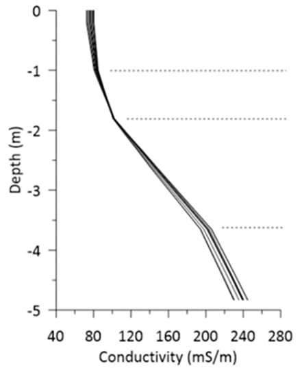
Figure 5.
Electrical conductivity profile around the coring site (within +/−2.5 m surface distance along with profile TST06.
Examples of field-wide conductivity distributions at three different depths (0.4, 2.3, and 4.6 m), resulting from the inversion of the collected geophysical data, are shown in Figure 6. The first two distributions (at 0.4 and 2.3 m) correspond to the upper and middle units and reflect a slight increase in conductivity from SW to NE (Figure 6). The third distribution, corresponding to the depth of 4.6 m is close to the maximum investigated depth and shows that soil conductivity is quite constant throughout most of the examined area. In Figure 7, we marked as an example, on profile TST02 (Figure 3 and Figure 4), the three different units: (a) the upper unit, at 0.0–1.0 m depth of conductivity <50 mS/m; (b) the middle unit at 1.0–2.5 m depth, of conductivity 50–150 mS/m; and (c) the lower unit, at 2.5–5.0 m depth and conductivity of >150 mS/s.
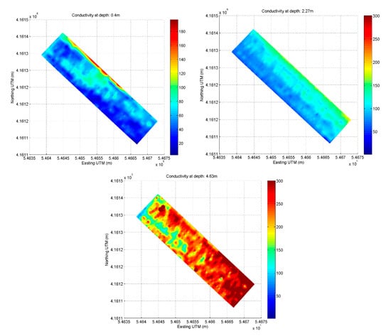
Figure 6.
Contour map of the electric conductivity in three different slices at depths of 0.4 m, 2.3 m, and 4.6 m.
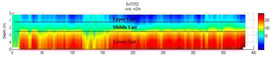
Figure 7.
Representative conductivity results for the transect EmTST02 of the studied field with the three sedimentological units.
The 3D model, obtained through INOBITEC software for core AG, presents variations that are attributed to changes in sediment physical properties (Figure 8). From 0.00 to 0.50 m, the core presents increased HU values that reflect higher density (Figure 8). Attaching HU boundaries on the 3D model and excluding the sediment in the studied volume reveals shell fragments in the unit as well as organic residues that were also macroscopically observed. From 0.50 to 1.00 m, the water-clogged organic-rich sediment presents decreased values of HU (Figure 8). This unit is also characterized by the lowest measured values of electrical conductivity. Variations in HU values and a completely different setting are observed from 1.00 to 4.00 m, with increased HU values, and organic residues and root remains are observed (Figure 8). This unit, composed mainly of sand, is also highly correlated with the increased values presented in the electrical conductivity profile.
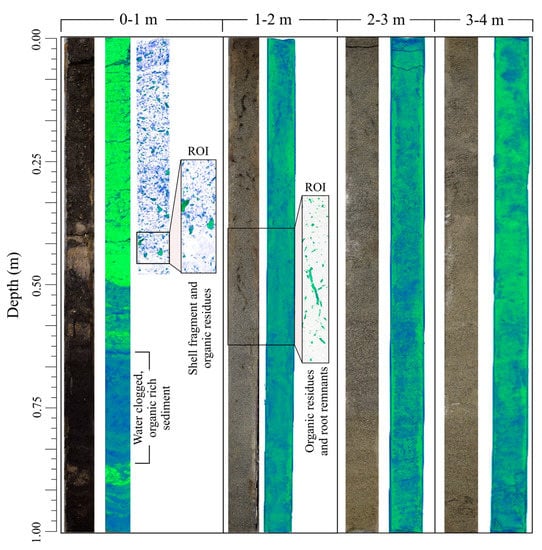
Figure 8.
Three-dimensional model of core AG with additional regions of interest (ROI) highlighted in boxes. Additional HU boundaries were attached in all regions in order to better visualize organic residues, shell fragments, etc.
5. Conclusions
We tested the combination of a classical sediment-core analysis (grain size and TOC) with CT and XRF detailed core investigation and soil electrical conductivity measurements in an area with a former marsh field in western Peloponnese. The core, site-specific analysis led to the identification of three sedimentological units with discrete textural and geochemical characteristics: (1) the upper, mostly silty-clay, unconsolidated and organic-rich unit (0–1 m) with characteristic low HU values; (2) the middle unit (~1–2 m) comprising mainly sand, with minor clay/silt content, with higher HU values, increased density, and considerable organic content; and (3) the lower unit (>~2 m). The latter presents a monotonous distribution of all studied parameters and differs from the middle unit in that it does not present any considerable amount of organic material.
The analysis was extended from site-specific to field-wide by applying an electromagnetic geophysical prospection along with nine parallel profiles, each of ~400 m length. The inversion of surface measurements of the soil’s apparent electrical conductivity provided a clear picture of the distribution of electrical conductivity throughout the investigated area, down to a depth of more than 4 m. Electrical conductivity showed a gradual increase with depth and analogue fluctuations with the sedimentological analysis at the site of the core sample, with the rate of increase changing at ~1 m and ~2 m. These changes are mild, and the increase with depth is smooth and continuous, which favours an interpretation linked to the increasing density of the soil material with depth. Similar distributions were derived for all nine examined profiles, supporting the extension of the site-specific core analysis to the entire investigated field.
Supplementary Materials
The following are available online at https://www.mdpi.com/article/10.3390/app11209575/s1, Table S1: Grain size values (sand, silt, and clay) and the TOC content measurements are also presented.
Author Contributions
Conceptualization, P.A. and P.B.; methodology, P.A., P.P. and A.E.; software, A.E., P.P. and Z.R.; validation, A.E., P.A. and Z.R.; data curation P.P., A.E. and Z.R.; writing—original draft preparation, P.A., A.E. and Z.R.; writing—review and editing, P.A.; supervision, P.A. and P.B. All authors have read and agreed to the published version of the manuscript.
Funding
This research received no external funding.
Informed Consent Statement
Not applicable.
Data Availability Statement
The data presented in this study are available on request from the corresponding author.
Acknowledgments
The authors thank Nikolaos Avrantinis, MSc Geologist, for the support in data acquisition in the field.
Conflicts of Interest
The authors declare no conflict of interest.
References
- Rothwell, R.G.; Rack, F.R. New techniques in sediment core analysis: An introduction. Geol. Soc. Lond. Spec. Publ. 2006, 267, 1–29. [Google Scholar] [CrossRef] [Green Version]
- St-Onge, G.; Mulder, T.; Francus, P.; Long, B. Chapter two continuous physical properties of cored marine sediments. In Developments in Marine Geology; Proxies in Late Cenozoic Paleoceanography; Claude, H., Anne De, V., Eds.; Elsevier: Amsterdam, The Netherlands, 2007; Volume 1, pp. 63–98. [Google Scholar]
- Weltje, G.J.; Tjallingii, R. Calibration of XRF core scanners for quantitative geochemical logging of sediment cores: Theory and application. Earth Planet. Sci. Lett. 2008, 274, 423–438. [Google Scholar] [CrossRef]
- Ketcham, R.; Carlson, W. Acquisition, optimization and interpretation of X-ray computed tomographic imagery: Applications to the geosciences. Comput. Geosci. 2001, 27, 381–400. [Google Scholar] [CrossRef]
- Coletti, G.; Stainbank, S.; Fabbrini, A.; Spezzaferri, S.; Foubert, A.; Kroon, D.; Betzler, C. Biostratigraphy of large benthic foraminifera from Hole U1468A (Maldives): A CT-scan taxonomic approach. Swiss J. Geosci. 2018, 111, 495–508. [Google Scholar] [CrossRef] [Green Version]
- Capowiez, Y.; Sammartino, S.; Cadoux, S.; Pierre, B.; Richard, G.; Boizard, H. Role of earthworms in regenerating soil structure after compaction in reduced tillage systems. Soil Biol. Biochem. 2012, 55, 93–103. [Google Scholar] [CrossRef]
- Zou, F.; Slatt, R.M. Relationships between Bioturbation, Microfacies and Chemostratigraphy and their Implication to the Sequence Stratigraphic Framework of the Woodford Shale in Anadarko Basin, Oklahoma, USA. In Unconventional Resources Technology Conference, San Antonio, Texas, 20–22 July 2015; SEG Global Meeting Abstracts; Unconventional Resources Technology ConferenceSociety of Exploration Geophysicists: Tulsa, OK, USA, 2015; pp. 1620–1638. [Google Scholar]
- Bendle, J.; Palmer, A.; Carr, S. A comparison of micro-CT and thin section analysis of Lateglacial glaciolacustrine varves from Glen Roy, Scotland. Quat. Sci. Rev. 2015, 114, 61–77. [Google Scholar] [CrossRef]
- Emmanouilidis, A.; Unkel, I.; Seguin, J.; Keklikoglou, K.; Gianni, E.; Avramidis, P. Application of non-destructive techniques on a varve sediment record from vouliagmeni coastal lake, eastern gulf of corinth, Greece. Appl. Sci. 2020, 10, 8273. [Google Scholar] [CrossRef]
- Romero-Ruiz, A.; Linde, N.; Keller, T.; Or, D. A Review of Geophysical Methods for Soil Structure Characterization. Rev. Geophys. 2018, 56, 672–697. [Google Scholar] [CrossRef] [Green Version]
- Corwin, D.; Lesch, S. Application of Soil Electrical Conductivity to Precision Agriculture. Agron. J. 2003, 95, 455–471. [Google Scholar] [CrossRef]
- Sudduth, K.; Drummond, S.T.; Kitchen, N. Accuracy issues in electromagnetic induction sensing of soil electrical conductivity for precision agriculture. Comput. Electron. Agric. 2001, 31, 239–264. [Google Scholar] [CrossRef]
- Williams, B.G.; Hoey, D. The use of electromagnetic induction to detect the spatial variability of the salt and clay content of soils. Aust. J. Soil Res. 1987, 25, 21–27. [Google Scholar] [CrossRef]
- Triantafilis, J.; Lesch, S. Mapping Clay content variation using electromagnetic induction techniques. Comput. Electron. Agric. 2005, 46, 203–237. [Google Scholar] [CrossRef]
- Doolittle, J.A.; Brevik, E.C.; Lincoln, N.; Doolittle, J.A.; Brevik, E.C. Digital Commons @ University of Nebraska—Lincoln The use of electromagnetic induction techniques in soils studies the use of electromagnetic induction techniques in soils studies. USDA-ARS/UNL Fac. 2014, 223–225, 33–45. [Google Scholar] [CrossRef] [Green Version]
- Kachanoski, R.G.; Wesenbeeck, I.J.V.A.N.; Gregorich, E.G. Estimating spatial variations of soil water content using noncanting electromagnetic inductive methods. Can. J. Soil Sci. 1988, 68, 715–722. [Google Scholar] [CrossRef]
- Wollenhaupt, N.C.; Richardson, J.L.; Foss, J.E.; Doll, E.C. A rapid method for estimating weighted soil salinity from apparent soil electrical conductivity measured with an aboveground electromagnetic induction meter. Can. J. Soil Sci. 1986, 66, 315–321. [Google Scholar] [CrossRef]
- Jaynes, D.B. Improved Soil Mapping using Electromagnetic Induction Surveys. Proc. Third Int. Conf. Precis. Agric. 1996, 169–179. [Google Scholar]
- Visconti, F.; de Paz, J.M. Sensitivity of soil electromagnetic induction measurements to salinity, water content, clay, organic matter and bulk density. Precis. Agric. 2021. [Google Scholar] [CrossRef]
- Emmanouilidis, A.; Messaris, G.; Ntzanis, E.; Zampakis, P.; Prevedouros, I.; Bassukas, D.A.; Avramidis, P. CT scanning, X-ray fluorescence: Non-destructive techniques for the identification of sedimentary facies and structures. Rev. Micropaleontol. 2020, 67, 100410. [Google Scholar] [CrossRef]
- Kraft, J.; Rapp, G.R.; Gifford, J.A.; Achenbrenner, S.E. Coastal change and archaeological settings in Elis. Hesperia 2005, 74, 1–39. [Google Scholar] [CrossRef]
- Haenssler, E.; Unkel, I.; Dörfler, W.; Nadeau, M. Driving mechanisms of Holocene lagoon development and barrier accretion in Northern Elis, Peloponnese, inferred from the sedimentary record of the Kotychi Lagoon. Quat. Sci. J. 2014, 63, 60–77. [Google Scholar] [CrossRef]
- Emmanouilidis, A.; Katrantsiotis, C.; Norström, E.; Risberg, J.; Kylander, M.; Sheik, T.A.; Iliopoulos, G.; Avramidis, P. Middle to late Holocene palaeoenvironmental study of Gialova Lagoon, SW Peloponnese, Greece. Quat. Int. 2018, 476, 46–62. [Google Scholar] [CrossRef]
- Weiberg, E.; Unkel, I.; Kouli, K.; Holmgren, K.; Avramidis, P.; Bonnier, A.; Dibble, F.; Finné, M.; Izdebski, A.; Katrantsiotis, C.; et al. The socio-environmental history of the Peloponnese during the Holocene: Towards an integrated understanding of the past. Quat. Sci. Rev. 2016, 136, 40–65. [Google Scholar] [CrossRef] [Green Version]
- Katrantsiotis, C.; Kylander, M.E.; Smittenberg, R.; Yamoah, K.K.A.; Hättestrand, M.; Avramidis, P.; Strandberg, N.A.; Norström, E. Eastern Mediterranean hydroclimate reconstruction over the last 3600 years based on sedimentary n-alkanes, their carbon and hydrogen isotope composition and XRF data from the Gialova Lagoon, SW Greece. Quat. Sci. Rev. 2018, 194, 77–93. [Google Scholar] [CrossRef]
- Seguin, J.; Bintliff, J.L.; Grootes, P.M.; Bauersachs, T.; Dörfler, W.; Heymann, C.; Manning, S.W.; Müller, S.; Nadeau, M.J.; Nelle, O.; et al. 2500 years of anthropogenic and climatic landscape transformation in the Stymphalia polje, Greece. Quat. Sci. Rev. 2019, 213, 133–154. [Google Scholar] [CrossRef]
- Avramidis, P.; Bouzos, D.; Antoniou, V.; Kontopoulos, N. Application of grain-size trend analysis and spatio-temporal changes of sedimentation, as a tool for lagoon management. Case study: The Kotychi lagoon (western Greece). Geol. Carpathica 2008, 59, 261–268. [Google Scholar]
- Katsaros, D.; Iliopoulos, G.; Panagiotaras, D.; Kontopoulos, N.; Avramidis, P. Geochemical and sedimentological assessment of the prokopos coastal lagoon sediments, mediterranean sea Western Greece. In Proceedings of the 15th International Multidisciplinary Scientific GeoConference Surveying Geology and Mining Ecology Management, SGEM, Albena, Bulgaria, 18–24 June 2015; Volume 2, pp. 249–256. [Google Scholar]
- Papatheodorou, G.; Avramidis, P.; Fakiris, E.; Christodoulou, D.; Kontopoulos, N. Bed diversity in the shallow water environment of Pappas lagoon in Greece. Int. J. Sediment Res. 2012, 27, 1–17. [Google Scholar] [CrossRef]
- Vött, A. Relative sea level changes and regional tectonic evolution of seven coastal areas in NW Greece since the mid-Holocene. Quat. Sci. Rev. 2007, 26, 894–919. [Google Scholar] [CrossRef]
- Obrocki, L.; Vött, A.; Wilken, D.; Fischer, P.; Willershäuser, T.; Koster, B.; Lang, F.; Papanikolaοu, I.; Rabbel, W.; Reicherter, K. Tracing tsunami signatures of the AD 551 and AD 1303 tsunamis at the Gulf of Kyparissia (Peloponnese, Greece) using direct push in situ sensing techniques combined with geophysical studies. Sedimentology 2018, 67, 1274–1308. [Google Scholar] [CrossRef]
- Vött, A.; Bruins, H.; Gawehn, M.; Goodman-Tchernov, B.; De Martini, P.M.; Kelletat, D.; Mastronuzzi, G.; Reicherter, K.; Rötbke, B.; Scheffers, A.; et al. Publicity waves based on manipulated geoscientific data suggesting climatic trigger for majority of tsunami findings in the Mediterranean—Response to ‘Tsunamis in the geological record: Making waves with a cautionary tale from the Mediterranean’ by Marriner et al. (2017). Z. Geomorphol. Suppl. Issues 2019, 62, 7–45. [Google Scholar] [CrossRef]
- Koster, B.; Vött, A.; Mathes-Schmidt, M.; Reicherter, K. Geoscientific investigations in search of tsunami deposits in the environs of the Agoulinitsa peatland, Kaiafas Lagoon and Kakovatos (Gulf of Kyparissia, western Peloponnese, Greece). Z. Geomorphol. 2015, 59, 125–156. [Google Scholar] [CrossRef]
- Willershäuser, T.; Vött, A.; Hadler, H.; Fischer, P.; Röbke, B.; Ntageretzis, K.; Emde, K.; Brückner, H. Geo-scientific evidence of tsunami impact in the Gulf of Kyparissia (western Peloponnese, Greece). Z. Geomorphol. Suppl. Issues 2015, 59, 43–80. [Google Scholar] [CrossRef]
- Institute of Geology and Mineral Exploration IGME. Nea Manolas Sheet, Athens. In Geological Map of Greece, 1:50000; Institute of Geology and Mineral Exploration: Athens, Greece, 1977. [Google Scholar]
- Institute of Geology and Mineral Exploration IGME. Pirgos Sheet, Greece. In Geological Map of Greece, 1:50000; Institute of Geology and Mineral Exploration: Athens, Greece, 1980. [Google Scholar]
- Maroukian, H.; Gaki-Papanastassiou, K.; Papanastassiou, D.; Palyvos, N. Geomorphological observations in the coastal zone of Kyllini Peninsula, NW Peloponnesus-Greece, and their relation to the seismotectonic regime of the area. J. Coast. Res. 2000, 16, 853–863. [Google Scholar]
- Fountoulis, I.; Vassilakis, E.; Mavroulis, S.; Alexopoulos, J.; Erkeki, A. Quantification of river valley major diversion impact at Kyllini coastal area (W. Peloponnesus, Greece) with remote sensing techniques. In Proceedings of the 2nd INQUA-IGCP-567 International Workshop on Active Tectonics, Earthquake Geology, Archaeology and Engineering, Corinth, Greece, 19–24 September 2011; pp. 46–49. [Google Scholar]
- Underhill, J.R. Late Cenozoic deformation of the Hellenide foreland, western Greece. GSA Bull. 1989, 101, 613–634. [Google Scholar] [CrossRef]
- Folk, R.L.; Ward, W.C. Brazos River bar [Texas]: A study in the significance of grain size parameters. J. Sedim. Res. 1957, 27, 3–26. [Google Scholar] [CrossRef]
- Walkley, A.; Black, I.A. An examination of the degtjareff method for determining soil organic matter and a proposed modification of the chromic acid titration method. Soil Sci. 1934, 37, 29–38. [Google Scholar] [CrossRef]
- Avramidis, P.; Nikolaou, K.; Bekiari, V. Total organic carbon and total nitrogen in sediments and soils: A comparison of the wet oxidation—Titration method with the combustion-infrared method. Agri. Agric. Sci. Proc. 2015, 4, 425–430. [Google Scholar] [CrossRef] [Green Version]
- Avramidis, P.; Bekiari, V. Application of a catalytic oxidation method for the simultaneous determination of total organic carbon and total nitrogen in marine sediments and soils. PLoS ONE 2021, 16, e0252308. [Google Scholar] [CrossRef]
- Reilly, B.T.; Stoner, J.S.; Wiest, J. SedCT: MATLABTM tools for standardized and quantitative processing of sediment core computed tomography (CT) data collected using a medical CT scanner. Geochem. Geophys. Geosystems 2017, 18, 3231–3240. [Google Scholar] [CrossRef]
- Rollinson, H. Using Geochemical Data: Evaluation, Presentation, Interpretation; Longman Scientific and Technical, Wiley: New York, NY, USA, 1993; p. 352. [Google Scholar]
- Monteiro Santos, F.A. 1-D laterally constrained inversion of EM34 profiling data. J. Appl. Geophys. 2004, 56, 123–134. [Google Scholar] [CrossRef]
- Ziegler, M.; Jilbert, T.; de Lange, G.; Lourens, L.; Reichart, G.-J. Bromine Counts from XRF Scanning as an Estimate of the Marine Organic Carbon Content of Sediment Cores. Geochem. Geophys. Geosystems 2008, 9, Q05009. [Google Scholar] [CrossRef]
- Shala, S.; Helmens, K.; Luoto, T.; Väliranta, M.; Weckström, J.; Salonen, J.; Kuhry, P. Evaluating environmental drivers of Holocene changes in water chemistry and aquatic biota composition at Lake Loitsana, NE Finland. J. Paleolimnol. 2014, 52, 311–329. [Google Scholar] [CrossRef]
- Burn, M.; Palmer, S.E. Solar forcing of Caribbean drought events during the last millennium. J. Quat. Sci. 2014, 29, 827–836. [Google Scholar] [CrossRef]
- Unkel, I.; Björck, S.; Wohlfarth, B. Deglacial environmental changes on Isla de los Estados (54.4°S), southeastern Tierra del Fuego. Quat. Sci. Rev. 2008, 27, 1541–1554. [Google Scholar] [CrossRef]
Publisher’s Note: MDPI stays neutral with regard to jurisdictional claims in published maps and institutional affiliations. |
© 2021 by the authors. Licensee MDPI, Basel, Switzerland. This article is an open access article distributed under the terms and conditions of the Creative Commons Attribution (CC BY) license (https://creativecommons.org/licenses/by/4.0/).