Hybrid Early Warning System for Rock-Fall Risks Reduction

Abstract

Rock-fall is a natural threat resulting in many annual economic costs and human casualties. Constructive measures including detection or prediction of rock-fall and warning road users at the appropriate time are required to prevent or reduce the risk. This article presents a hybrid early warning system (HEWS) to reduce the rock-fall risks. In this system, the computer vision model is used to detect and track falling rocks, and the logistic regression model is used to predict the rock-fall occurrence. In addition, the hybrid risk reduction model is used to classify the hazard levels and delivers early warning action. In order to determine the system’s performance, this study adopted parameters, namely overall prediction performance measures, based on a confusion matrix and reliability. The results show that the overall system accuracy was 97.9%, and the reliability was 0.98. In addition, a system can reduce the risk probability from (6.39 × 10⁻³) to (1.13 × 10⁻⁸). The result indicates that this system is accurate, reliable, and robust; this confirms the purpose of the HEWS to reduce rock-fall risk.

1. Introduction

Rock-fall on the roads causes a severe threat to transportation systems. The risk of landslides and the fall of rock blocks in Saudi Arabia’s mountains have caused many problems, and these geological hazards can occur at any moment. The level of risk is due to several circumstances such as natural factors due to weakness in the mountain crust, rocky rubble, and tectonic movements and their relationship to the lines of weakness and structural characteristics of cracks, as shown in Figure 1a,b.

Other factors are due to construction and development work, such as poor road construction, poor drainage methods of torrential rains, and erosion as a result of floods [1]. Figure 1c,d illustrates some examples of these types of artificial problems [2,3]. All these risk factors integrate with the natural disasters that are difficult for humans to prevent because the risks are not within the human potential to predict, and using a conventional ground survey is not sufficient to inform a geological hazards map.

Modern techniques have been used to detect risks and mitigate the destructive impact of all the aforementioned risk factors. There are two methods used to reduce the risks of the phenomenon of rock-fall, either by simulation and modeling (semi-real time) or by detection and monitoring of the fall event (in real time).

There are several approaches reported in the literature to model rock-fall behavior. For example, references [4,5] developed a stochastic impact model to calculate the velocities of a falling rock after a rebound on the slope. Another study [6] discussed probability distributions of rock-fall velocities and volumes to calculate kinetic energy distribution. A further possibility to model rock-falls is to use historical information from past rock-fall events and field surveys [7]. However, the above studies suffered from uncertainties in the field surveys and the randomness of natural variables. Therefore, additional information was used to overcome the limitations, such as the rebound value of both the block and the slope material, the impact velocity, and the block mass [8]. In addition to the assessment of rock slope stability with the effects of weathering, the rock was modeled by some shear properties (such as resistance, displacement, incident velocity, and stress along the rocks’ interconnecting areas [9,10,11,12].

Several approaches are reported in the literature to model several assessment methods that evaluated rock-fall hazards. For example, reference [13] proposed a hazard rating model based on rock-fall frequency and bounce height. In addition to rock structure, the proposed model, the rock-fall hazard, and the uncertainties in quantification were assessed by dynamic computational methods. In another pair of studies, quantitative rock-fall risk models were developed to assess the rock-fall risk using a model to identify and manage the risk [14,15]. In addition, there are many approaches to determine the conditions of a rock-fall trajectory and to simulate its behavior. One of these approaches is the kinematic study of the motion of blocks, in which the coefficients of restitution are calculated, and the other approach is the propagation history of rocks, which has been used to determine the characteristic impact conditions and to verify the mode of motion of rock blocks [16]. Another possibility to simulate the trajectories is discontinuous deformation analysis, which describes the rock-fall trajectories and the motion behaviors as bouncing, rolling, free falling, and sliding [17]. Furthermore, reference [18] conducted a review of the various probabilistic modeling models and found that most models were not systematic because the probabilistic variables were randomly sampled from the probability distributions.

There are different techniques reported in the literature to monitor seismic signals caused by falling rocks. First, geophysical sensors were proposed to monitor the geophysical signals induced by the falling rocks and estimate the impact of the fall of the rock on the surface [19]. In another study [20], a micro-seismic technique was presented to detect rock-fall events. However, these techniques detect rock-fall events but are unable to locate the fall. New techniques were proposed to overcome micro-seismic limitations [21,22,23] by locating rock-fall impacts using micro-electromechanical and micro-seismic networks with highly dynamic ranges. Several techniques are reported in the literature [24,25,26], where a terrestrial laser scanner was used to detect changes occurring on the surface as well as to detect individual rock events. To detect multiple rock-fall events, semi-automated identification methods were used, capable of extracting information from events of rock-falls, including block shapes, volumes, and their locations [27]. In addition, [28] proposed a semiautomatic method in which three-dimensional terrain was reconstructed to obtain the geometry of the unstable blocks and to define the location of rock-fall source areas.

Although few camera-based rock-fall monitoring techniques were found in the literature, the camera has outperformed many technologies, even the terrestrial laser scanner, regarding its ability to track multiple rocks in real time. In Fantini et al. [29], an artificial intelligence camera prototype was used for monitoring and tracking the fallen rocks in real time. All the above methods are used to detect falling rocks; however, they are not sufficiently effective to warn cars of rock-fall hazards before their occurrence. These methods respond after the rock-fall occurrence has caused harm on the roads. In addition, they have weak capabilities in dealing with the high falling speed and the slow response of the vehicle’s driver that increases the risk. A prediction of rock-fall events is required to address the shortcomings of previous models. Recently, machine learning technologies have been used in developing effective models to predict rock-fall hazards. Some studies were conducted on rock-fall prediction models based on machine learning technology [30,31,32]. The existing methods are unreliable in mitigating the rock-fall risk in real time because the model is generated from the historical data concerning a specific site.

Moreover, few studies focused on increasing the reliability of the detection or the prediction models. Therefore, this study aimed to increase the reliability by combining the detection and the prediction models in a hybrid reliable early warning system that guarantees to overcome the limitations of existing technologies and make the roads safer. Therefore, the key contributions of this study are summarized as follows:

• We developed a prediction model-based machine learning technology to predict the possibility of rock-fall.
• We developed a detection model-based computer vision algorithms to detect and track rock-fall events.
• We combined the detection and the prediction models in a hybrid reliable risk reduction model to increase the model reliability.
• We developed a hybrid early warning system to reduce the rock-fall risks.

The rest of this study is organized as follows. The study area and problems are presented in Section 2. The system platform and the methodology are introduced in Section 3. The proposed system validation is presented in Section 4. Section 5 presents the discussion and the conclusion of the study.

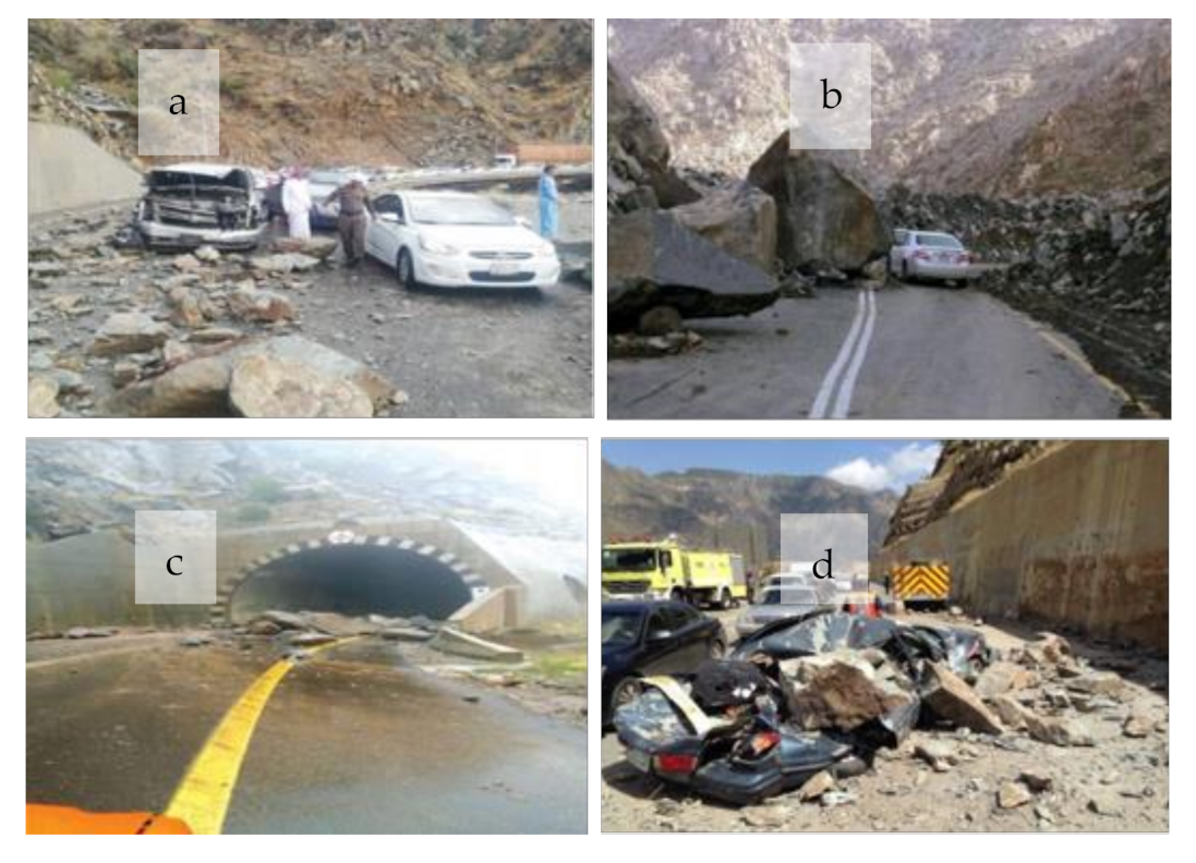
2. Study Area and Problems

The Aqbat-Shaar in the region of Asir in Saudi Arabia is one of the gigantic projects established more than 25 years ago and includes 11 tunnels along 32 bridges over 65 m high and about 351 drainage ferries. The Aqabat-Shaar linked Sarat Asir to its charge and reduced the journey time for travelers. The biggest concern is disrupting the people passing through the crowded trucks with bends and tunnels, especially on weekends and vacations. The slogan obstacle is the only outlet for trucks that connects Tihama Asir with its Saratha, and Aqabat is crowded with small cars in addition to trucks, and then many tragic accidents happen and the area becomes littered with corpses [33]. The affected road rock-fall is 0.6 km out of the 49.8 km road that is partly single lane from Muhaial to Abha city. On this road, the average speed is 86.1 km/h, and the daily average vehicle rate is 6245. There is a peak hour mainly during the morning and a rush hour during the night, the first at 07:00 for a limit of 320 cars and the second at 15:00, when the total number of vehicles reaches 320 vehicles. The partial collapse phenomenon at the Aqabat Shaar of Asir Region was studied by the Saudi Geological Survey to find out the causes of this collapse and ensure there are no consequences for other collapses in the same area [34].

The report issued by the working group assigned to study this phenomenon indicated that one of the most important reasons for this collapse was a crack at the top of the collapsed rock slope. This crack widened with time due to various factors, including ground movements or the action of water pools inside fissures due to rainwater, as the porosity in these rocks is high. In addition, the absence of rainwater drains in the concrete barrier caused pressure inside the rock cracks, which caused a decrease in the strength of cohesion between the blocks and thus led to loosening and collapse. In addition, the various weathering factors, whether mechanical or chemical, that work on weathering the rocks play an essential role in reducing the strength of the rock’s resistivity, making it weak, fragmented, and vulnerable to collapse [35], as illustrated in Figure 1.

3. Data Used

Past rock-fall evidence is a crucial element in the estimation of possible events. In this study, two of the sites most plagued by rock-fall injuries were identified and approved as a study location. The rock-fall positions such as inventory reports and field surveys were described by two approaches. Three sources were used to collect historical data on rock-fall and their related weather information databases: Geological Hazards Research Center, KSA Civil Defense, and General Authority of Meteorology and Environmental Protection. From January 2015 to December 2018, a total of 75 rock-fall accidents were registered, and date of occurrence, location, and weather data were stored for each. The period was broken into 192 equivalent sampling intervals to incorporate a non-rock-fall event into the data collection. Then, the value assigned to the survey period in which rocks existed was one; otherwise, it was assigned as zero. The rock-fall inventory data were separated into two subsets for research purposes—a training data set of 65% (134 samples of 54 rock-falls) and a test data set of 35% (58 samples with 21 rock-falls). For the generation of rock-fall models, the training and the testing data sets were used for model validation. One dependent variable (rock-fall event) and three independent variables (rainfall rate, temperature variation, and slope angle) were derived during the inventory data review. In the study of rock-fall incidence, three contributing factors were considered based on the available evidence and literature review [36,37]. These variables include weather variables (rainfall intensity, temperature difference) and spatial variables (slope angle). The rainfall rate is a major rock-fall initiating factor [38]. The study area consists of rubble layers, boulders, and small rocks. The geological composition of mountains induces heavy rainfall to shift debris layers, contributing to rock movement and dropping. The fluctuations in temperature have an apparent effect on the rocks’ stability. Cyclical variations in temperature allow rock surfaces to expand and compress, leading to deformation or rock cracks [39]. The angle of the slope has an apparent effect on susceptibility to rock-fall. The higher the angle of the slope is, the less stable the rocks are [40].

4. Methodology

This section presents an overview of the proposed hybrid early warning system (HEWS) to reduce the rock-fall risk using computer vision and machine learning. The system is composed of three sub-models: detection, prediction, and hybrid risk reduction models. The following subsections give details of the system implementation and validation.

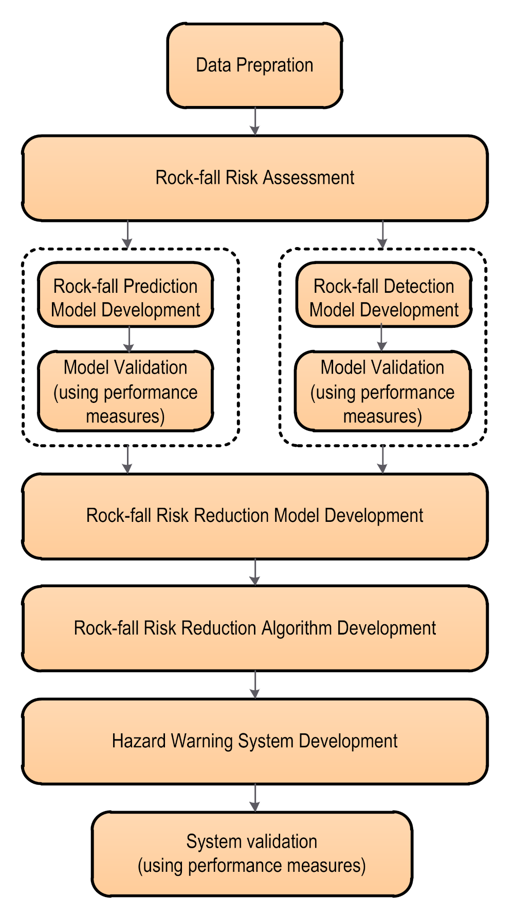
4.1. Overall Methodology

The approach applied was completed in five steps (Figure 2). First, rock-fall incident data, related traffic data, and weather information were collected and prepared for analysis and variables selection phase. Then, the rock-fall risk was assessed based on the given data. Next, the rock-fall prediction model was developed based on the impact of independent variables (rock-fall influencing factors) on the dependent variable (occurrence of rock-fall). Overall performance measures validated the model. The model was developed and evaluated using SPSS V.22 software. After, the rock-fall detection model was developed and validated. Afterwards, the hybrid risk reduction module was developed. Finally, the hybrid hazard warning system platform was implemented and validated.

4.2. Rock-Fall Risk Assessment

The rock-fall risk is characterized as the possibility of a rock-fall phenomenon occurring in a particular space and time causing a specific degree of harm to road infrastructure, vehicles, and pedestrians [41]. Vehicles are known to be the targeted priorities on the highway in this analysis. The risk was calculated by integrating the likelihood that the fallen rocks will hit the vehicle, the temporal–spatial probability, and the susceptibility. In this paper, the likelihood of rocks falling is calculated based on the possibility that vehicles are presenting a specific position and period affected by rocks falling [42]. The rock-fall risk is determined utilizing a probability equation that combines the probability of the occurrence, the temporal and the spatial probabilities, and the vulnerability. The value of the risk probability is presented in Equation (1).

$$P_{\left(Risk\right)}=f_h\times P\left(r\right)\times P\left(S:T\right)\times V\left(D:T\right)$$

(1)

where $P_{\left(Risk\right)}$ is the risk probability of rock-fall, f_h represents the rock-fall frequency, and it is the likelihood of a rock-fall incident occurring during one hour. P(r) is the possibility that the fallen rocks will hit the vehicle on the road. V(D:T) is the vulnerability of the vehicle regarding rock-fall incidents. It takes two values: 1 in the case of a rock hitting the vehicle or 0 otherwise. P(S:T) is the temporal–spatial probability, which is the possibility that vehicles are present in a specific position and time.

It is a probability that a vehicle occupying the length of the path is affected at the time of effect (temporal–spatial probability). This is measured according to Equation (2) [43]:

$$p_{\left(S:T\right)}=\frac{N_V}{24}\times \frac{L_v}{1000}\times \frac{1}{V_v}$$

(2)

where N_v = is the average number of vehicles per day, L_v = is the average vehicle length in meters, and V_v = is the average vehicle speed (km/hour).

4.3. Rock-Fall Prediction Model Development

The machine learning technique was used to develop a prediction model. For this study, logistic regression was selected because it is helpful in estimating the occurrence or the absence of a consequence dependent on the values of predictor variables. The benefit of logistic regression is that the variables, or any combination of all forms, may be continuous or discrete, and the data do not need a regular distribution [44]. A rock-fall event was used in this analysis as a dependent variable (binary) describing the rock-fall event occurring or not occurring with values between 0 and 1. The logistic regression method yields coefficients for each independent variable based on data samples taken from a training dataset of 134 samples (65% of rock-fall inventory). In a mathematical function, these coefficients act as weights used in the decision-making algorithm to produce likelihood and risk level of rock-fall incidence. The logistic regression function used to determine the likelihood of rock-fall occurrence is expressed in the following Equation (3):

$$\mathrm{p}\left(\mathrm{r}\right)=\frac{e^{\left({\beta }_0+{\beta }_1{x}_1+{\beta }_2{x}_2+\cdots +{\beta }_n{x}_n\right)}}{1+e^{\left({\beta }_0+{\beta }_1{x}_1+{\beta }_2{x}_2+\cdots +{\beta }_n{x}_n\right)}}$$

(3)

where $\mathrm{p}\left(\mathrm{r}\right)$ refers to rock-fall occurrence probability, ${\beta }_0$ represents the intercept of model, ${\beta }_i\left(i=1,2,\dots ,n\right)$refers to the model coefficients, and$x_i\left(i=1,2,\dots ,n\right)$ represents the independent variables. The constant ${\beta }_0$ and the coefficients ${\beta }_i$ refer to compute and estimation of maximum likelihood [45]. The computation was performed based on the values of the independent variables and the condition of the dependent variable [46]. The model was validated by using overall performance measures dependent on an uncertainty matrix.

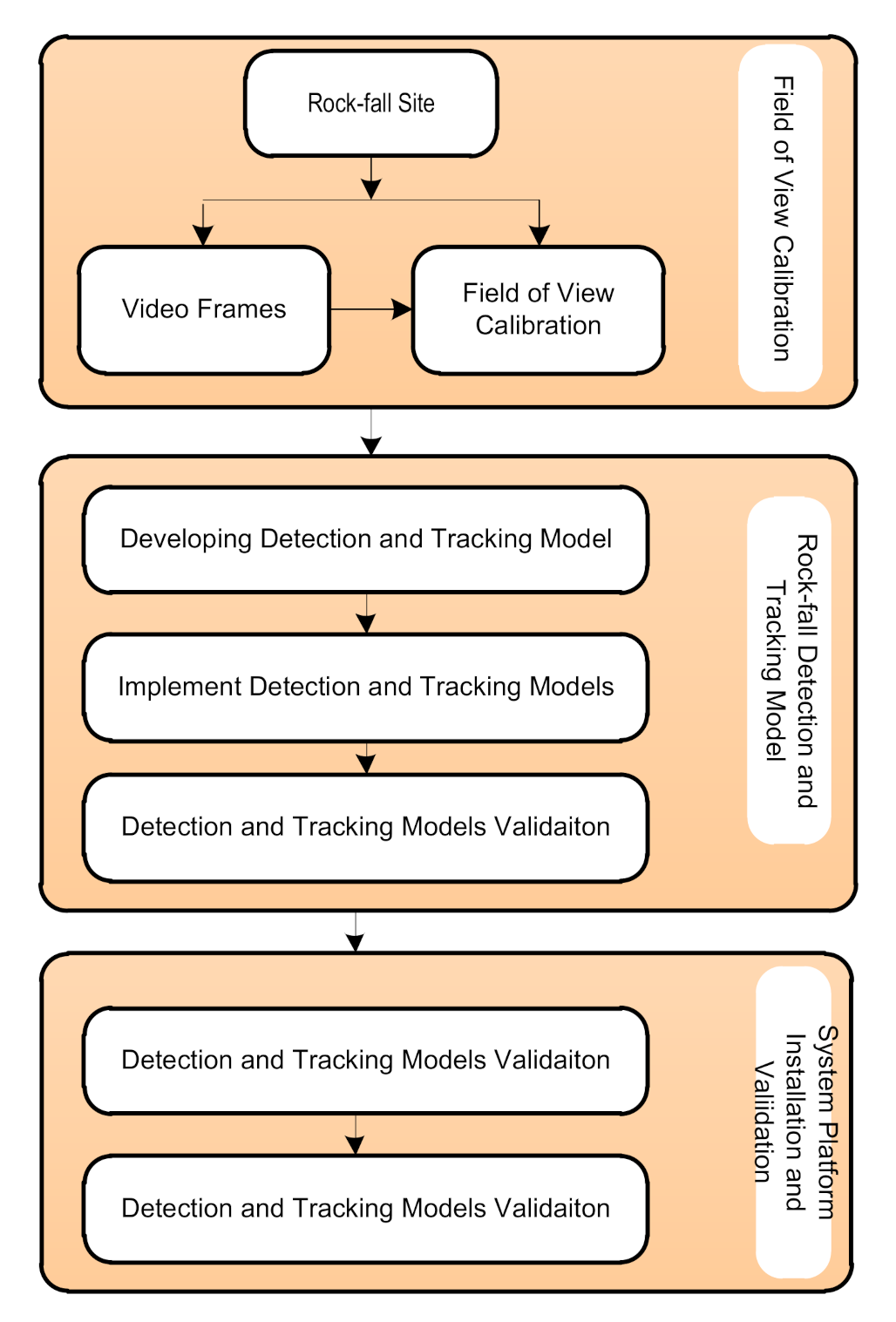
4.4. Rock-Fall Detection Model Development

This section describes the methodology strategy used to develop and validate the rock-fall detection model. The strategy applied was completed in three steps. First, the field of view was calibrated. Next, the detection model was developed by computer vision algorithms. Finally, the model was installed and validated. Figure 3 shows the general view of the detection model development steps.

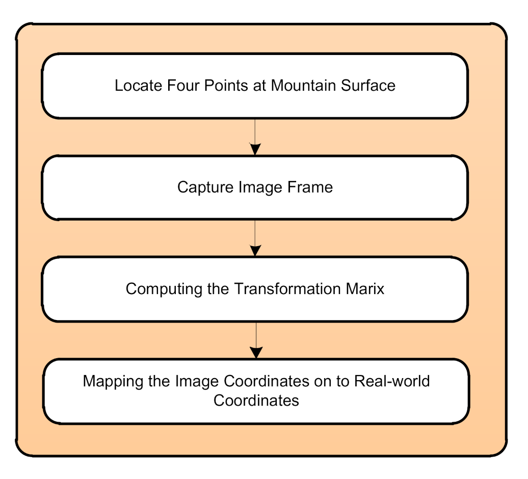
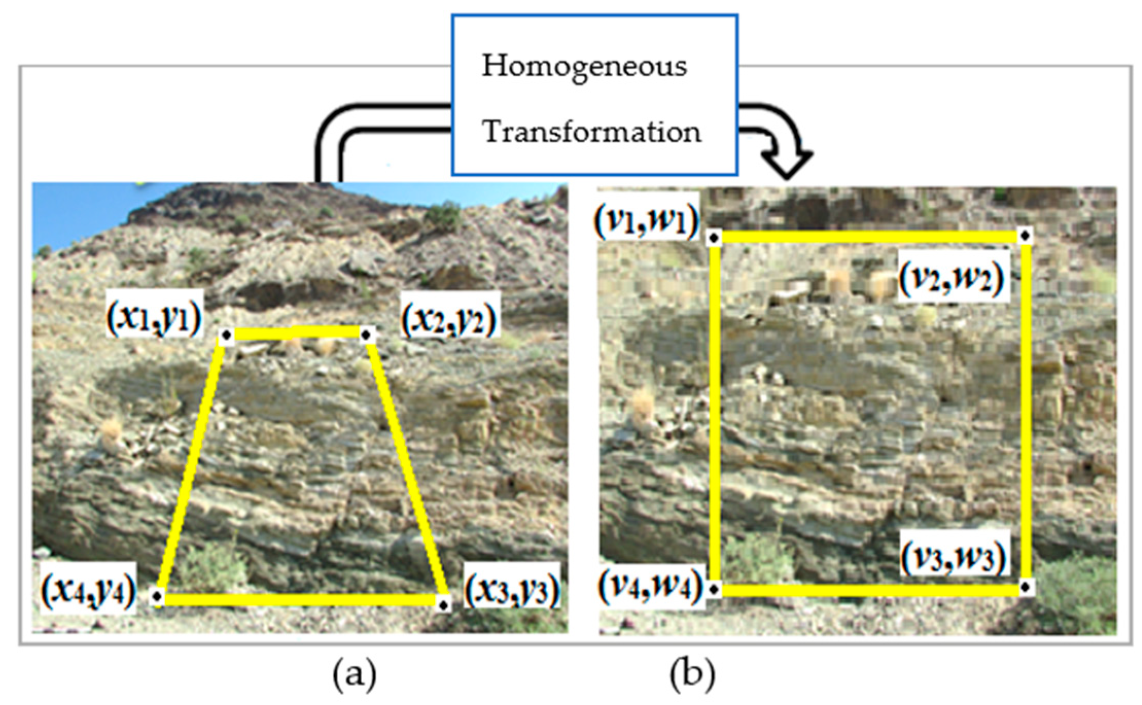
Field of View Calibration

The field of view calibration process was carried out through a linear transformation from an image coordinate system to a real world coordinate. The linear transformation projects any point on the image to a single location on the real world coordinate mountain through the perspective view transformation [47]. In addition to the coordinate transformation process, the perspective distortion is also corrected at this stage [48]. This process goes through four stages, as shown in Figure 4.

First, four calibration points, (x₁, y₁), (x₂, y₂), (x₃, y₃), and (x₄, y₄), were manually placed at the mountain surface. Second, the distorted image was captured, and the calibration points were detected in an image. Third, the transformation matrix was calculated by using the plane homographic method [41]. This method computes the transformation matrix by projecting points from the image plane into four points, (v₁, w₁), (v₂, w₂), (v₃, w₃), and (v₄, w₄) in world plane, which forms a rectangle plane as illustrated in Figure 5. Finally, the transformation matrix was used to map all points from image coordinates to real-world coordinates. The plane homograph was used to remove the projective distortion from a perspective image, as seen in Figure 5a [47]. The homogeneous transformation matrix was introduced to apply perspective rotation and scaling in the perspective image. Figure 5b shows the image after correction.

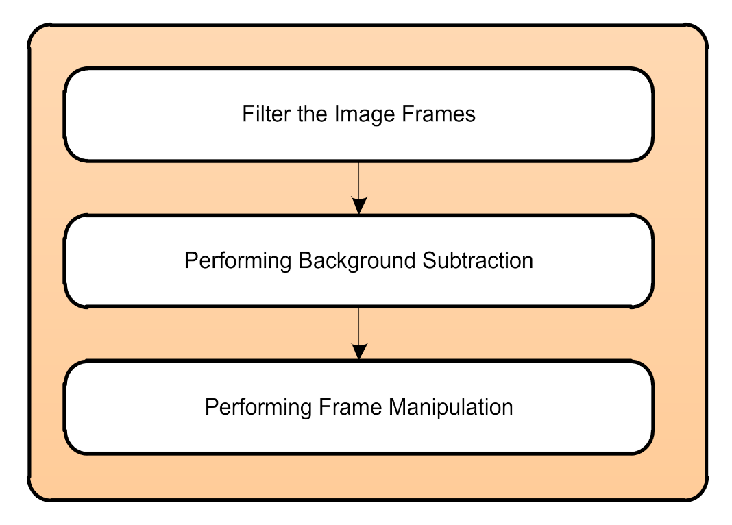
4.5. Rock-Fall Detection Process

The rock-fall detection process occurs in three stages, filtering the image frame, background subtraction, and performing frame manipulation, as in Figure 6. Firstly, the blurring Gaussian filter was used to cancel out the noise from captured images. This noise was caused by swing weeds and tiny drops of rain. Secondly, the adaptive Gaussian mixture model was used to detect moving rocks in a sequence of a video frame that suffered from variations in the background illumination due to time of day and weather conditions.

The model values a particular pixel as a mixture of Gaussians and performs two tasks: learning the background model and classifying pixels as background or foreground. Equation (4) represents the background model.

$$\widehat{P}\left(\overrightarrow{x}|{\chi }_{T },BG\right)={{\displaystyle \sum }}_{m=1}^M{\widehat{\pi }}_m\mathcal{N}\left(\overrightarrow{x};{\widehat{\overrightarrow{\mu }}}_m,{\widehat{\sigma }}_m^{2}I\right)$$

(4)

where $\widehat{P}\left(\overrightarrow{x}|{\chi }_{T },BG\right)$ is the background estimated, $\overrightarrow{x}$ is value of a pixel at time t in grayscale color space, ${\chi }_T$ is a training set, M is the number of the Gaussian components, πm is a weight that describes how much of the data belong to the m component of the GMM, ${\widehat{\overrightarrow{\mu }}}_m$ is estimates of the means, ${\widehat{\sigma }}_m^2$ is estimates of the variances, and I is the identity matrix.

The moving rocks were considered as foreground clusters of pixels. A Bayesian decision was introduced to classify pixels as background (BG) or foreground (FG), which is comparing a background estimated value of a particular pixel with the threshold; if it is greater than the threshold, it is considered a background, otherwise, it is considered a foreground [49]. To track a continuous change in the image of the scene, the model updates the training data set at every reasonable period T and re-estimates the background model value. After the foreground pixel cluster is classified and segmented from a background, holes appear in the foreground due to imperfection introduced during segmentation. The dilation process was used to fill in those holes, and it is one of the morphological image processing tools which adds pixels to the boundaries of objects in an image.

4.6. Hybrid Risk Reduction Model

The proposed model combines the output of detection and prediction models to issue an early warning. The model decreases the vulnerability of vehicles to risk by alerting vehicles before approaching the threat zone at the time of the rock-fall incident. The rock-fall risk reduction was assessed based on the possibility that vehicles will not reach the hazard zone after receiving the early warning signal at the time of the incident [50]. In this study, the risk reduction value was determined by a probability equation that combines the probability of vehicle response, the system reliability, and the average number of vehicles. The following Equation (5) indicates that:

P_(Reduction) = N_v × R_(h) × P_(response)

(5)

where P_(Reduction) is the risk reduction probability, P_(response) is the probability that a given vehicle does not reach the affected road segment after receiving the warning signal, N_v is the average number of vehicles, and R_(h) is the hybrid model reliability. The overall reliability of the two detection and prediction models connected in parallel is calculated according to Equation (6) [51]:

R_(h) = 1 − (1 − R_(d)) × (1 − R_(p))

(6)

R_(d) is the reliability of the detection model, and R_(p) is the reliability of the prediction model. The P_(response) can be calculated according to Equation (7):

$$P_{\left(response\right)}=1-\left(\frac{Total Stopping Distance}{Safe Distance to Stop}\right)$$

(7)

The total stopping distance was measured by combining reaction time, brake contact distance, and physical force distance. The safe distance to stop is the reaction interval that passes until the brakes are applied. It was evaluated by multiplying the vehicle velocity by the driver reaction time.

The driver reaction time is the reaction interval that passes until the brakes are applied. It takes a random value between 0.4 and 2 s [52]. When the physical force distance travels a distance after the brakes are engaged, it can be determined by multiplying vehicle speed by brake reaction time.

4.7. Risk Reduction Algorithm

The rock-fall risk reduction algorithm was developed to perform the rock-fall risk reduction process. It computes the rock-fall hazard, classifying it into three levels and generating an early warning action to reduce the risk of a critical situation. The following steps show how the presented Algorithm 1 determines a rock-fall hazard level and manages it.

Algorithm 1. To compute a rock-fall risk, classifying the risk level, and performing the rock-fall risk reduction action

Step 1: Inputs

Read (video frames from camera)

Read (weather data from sensors)

Step 2: Detect the moving rocks$\widehat{\mathrm{P}}\left(\overrightarrow{\mathrm{x}}|{\mathsf{\chi }}_{\mathrm{T} },\mathrm{BG}\right)$:

according to Equation (6)

Step 3: Predict the rock fall event p(x):

according to Equation (2)

Step 4: Compute the rock fall risk $P_{\left(Risk\right)}$

according to Equation (3)

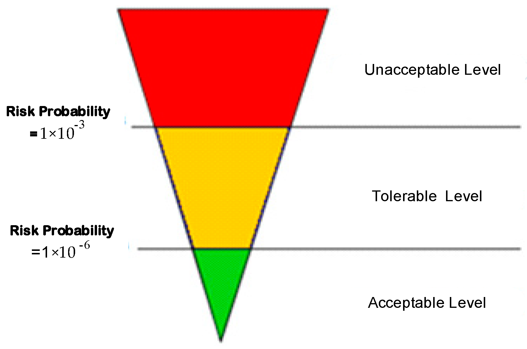
Step 5: Classify the hazard level:

Classifying the hazard level in to three levels

if ($P_{\left(Risk\right)} \ge 1\times {10}^{-3}$)

then Unacceptable level

if ($P_{\left(Risk\right)}>1\times {10}^{-6} and<1\times {10}^{-3}$)

then Tolerable level

if ($P_{\left(Risk\right)}$$\le 1\times {10}^{-6}$)

then Acceptable level

Step 6: Perform the rock-fall risk reduction action

Generate light and sound alarms

in case of   Unacceptable level   (Red light+ sound)

in case of   Tolerable level   (Yellow light)

in case of   Acceptable level   (Green light)

Save (x1, x2, x3, p(x)) every 30 min

Step 7: Return to Step 1

4.8. Hybrid Early Warning System

The proposed hybrid early warning system (HEWS) was implemented with a platform that combines hardware and software components.

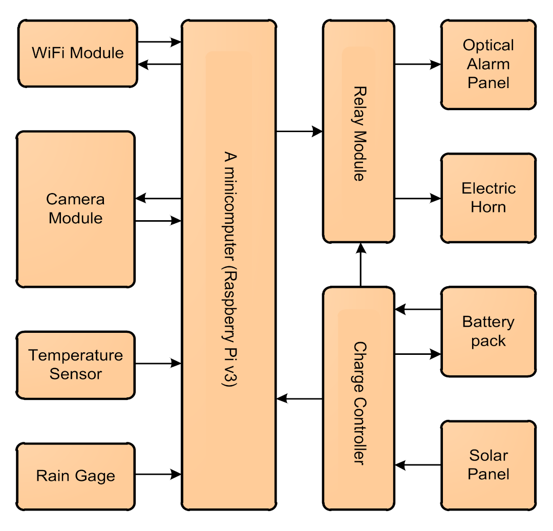
4.8.1. Hardware Components

Figure 7 illustrates the proposed system block diagram, and it defines the relationships of the hardware components and their features. It receives input through weather sensors and cameras, and its output is displayed through an optical panel and the electric horn.

A minicomputer (Raspberry Pi v3) was used to perform device computations, which appear in the central part of this graph. The minicomputer was fitted with USB ports, digital ports, and analogue ports. This single-board machine enables sensors and other devices to be connected. The left part of this diagram shows a temperature sensor and a rain gage. The temperature sensor is used to measure surrounding air temperature and generate a digital signal every two seconds (0.5 Hz sampling rate). The rain gauge is a tipping-bucket rain scale used with a resolution of 0.1 mm per tip to measure instantaneous rainfall. The one bucket tip produces one electrical signal (pulse).

There are four devices in the right part: the light warning screen, the relay module, the electric horn, and the WIFI module. The light warning panel is a 24 × 24 cm frame with an RGB LED matrix with high light strength. Suppose each color depends on the particular degree of hazard: this panel shows the warning light alert in three different colors (green, black, and red). The relay module consists of a photoelectric coupler with anti-interference insulating capacity. It supports the Raspberry Pi by general purpose input/output (GPIO) pins to drive the electric horn and the optical screen.

The bottom section of this graph displays the power system used during the day to maintain electrical power. It consists of a solar panel, a battery pack, and an intelligent solar charge controller. The solar panel transforms photo power into electrical energy. During hours of darkness, the battery pack is a backup power source for the device. The intelligent solar charge controller was used to supply the device and refresh the tank.

4.8.2. Software

Raspbian Stretch (GNU/Linux 9.1) was used as the operating system for a minicomputer module. This module utilizes the four cores of the ARM Processor to work in parallel. The main program was implemented in Python (version 3.5) scripts. Furthermore, it was compiled on-board with dedicated compilers. Python Multiprocessing Module was used to improve system response and computation performance. The falling rocks detection process was implemented by using an open computer vision module (open CV). The statistical analysis was performed using SPSS software (version 22).

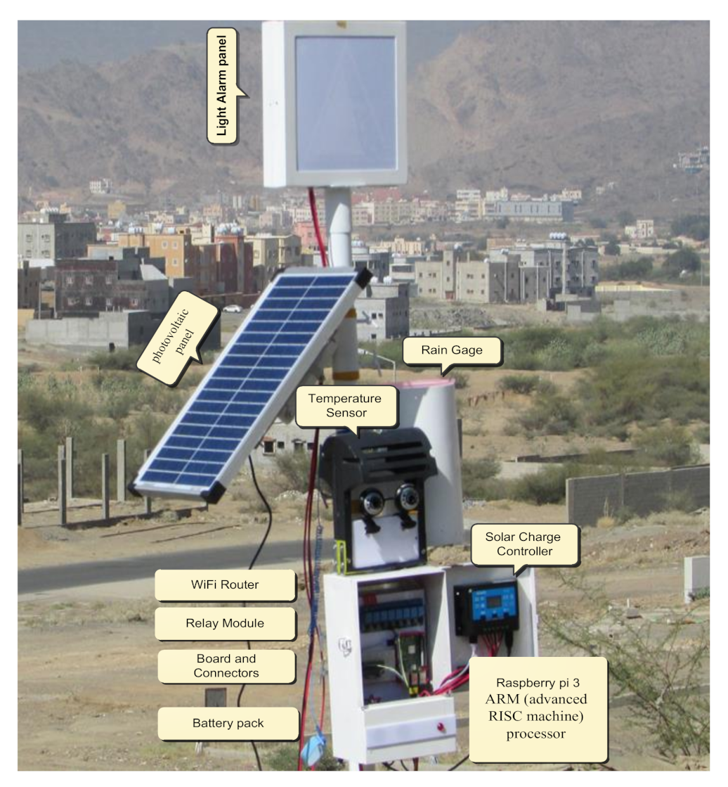
4.8.3. Platform Installation

The hybrid early warning system platform was installed in a vertical metal stand with a height of 240 cm; a stand-alone solar-powered system carried main system case, rain gauge, light alarm panel, cameras, and photovoltaic panel as shown in Figure 8.

4.9. System Validation

This section summarizes the validation metrics used in system validation. The proposed system was validated using four performance measures: sensitivity, specificity, accuracy, and reliability. The first measure is sensitivity, which reflects the ability of the system to detect the rock correctly, calculated as [53]:

$$Sensitivity=\frac{TP}{TP+FN}\times 100\%$$

(8)

The second measure is specificity. This reflects the ability of the system to confirm the absence of a rock-fall event, which is defined as:

$$specificity=\frac{TN}{TN+FP}\times 100\%$$

(9)

The third measure is accuracy. This reflects the accuracy of the system in detecting a rock-fall event, which is defined as:

$$Accuracy=\frac{\left(TP+TN\right)}{\left(TP+FN+TN+FP\right)}\times 100\%$$

(10)

The last measure is reliability, which reflects the degree of measure consistency when repeating result N times under the same conditions, which is defined as:

$$Reliability=\frac{1}{N}{\displaystyle \sum }_{i=1}^N\left(Accuracy \mathrm{at} \mathrm{Test}\left(\mathrm{i}\right) \right)$$

(11)

where true positive (TP) means all events were true detected, false negative (FN) means some events occurred but were not detected, true negative (TN) means events were absent and the system reports an absent event, and false-positive (FP) means the events were absent but the system reports it as present.

5. Results and Discussion

This section presents the results along with a discussion of these results. The results of the experiment demonstrate four things. First is the risk assessment. The second is the rock-fall prediction model experimental results. Third is the rock-fall detection model experimental results, and the last is the rock-fall risk reduction.

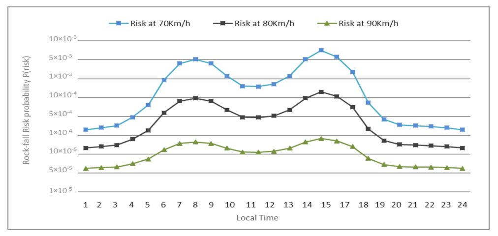
5.1. Risk Assessment

After data were picked up from the historical data of the rock-fall accidents and the traffic flow dataset, we used a Python environment to simulate the risk of falling rocks. The configurations and the setups that were used for simulation are shown in

Table 1. Simulation setups.

Parameter	Value
Average vehicle lengths	5.4 m
Average number of vehicles driving on the road every day (NV)	6245 vehicles
Average vehicle speed range (Vv)	70 to 90 Km/h
Vulnerability of the vehicle regarding rock-fall incidents V(D:T)	1
Rock-fall frequency (fh)	0.07 Per day

:

The rock-fall risk values, $P_{\left(Risk\right) }$, were tested for three different vehicle speeds of 70 km/h, 80 km/h, and 90 km/h, the results ranging from (6360 × 10⁻⁵) to (6386 × 10⁻³), as seen in Figure 9. The obtained results were compared with the safety-critical regulation and management as low as reasonably practicable (ALARP) thresholds triangle to classify the risk into levels. ALARP criteria were used to define three levels of a rock-fall risk, and Figure 10 shows the ALARP thresholds triangle [54].

By comparing the rock-fall risk values with the three levels of the ALARP thresholds triangle, we found that 86% took values more significant than (1 × 10⁻³) and thus were within an unacceptable level. The remaining 14% of risk values fell less than (1 × 10⁻³) and thus were spread between tolerable and acceptable levels.

5.2. Prediction Model Results

SPSS V.22 program was used to implement a prediction model to assess the rock-fall occurrence–rock-fall influencing factors relationship. The parameters of the model and their significant probabilities are shown in

Table 2. Prediction model parameters.

Independent Variable	Coefficient (β)	Std. Error	Wald	Significant Probability
Slope-angle	0.306	0.132	5.419	0.020
Rainfall-rate	0.425	0.165	6.669	0.010
Temperature variation	0.915	0.421	4.712	0.030

Std. Error = standard error of coefficient, Wald = Wald statistics.

.

From the data in Table 2, the standard error values (Std-Error) were less than 0.5, which were deemed tiny, indicating how similar the forecasts were to the eventual results. The likelihood of importance is another parameter that emerged in Table 2. This parameter confirmed the independent causes that had a significant effect on a rock-fall. If the significant likelihood was less than 0.05, this meant that the independent variable in rock-fall was statistically significant [21]. The findings revealed that slope angle, precipitation rate, and temperature variation with large likelihood values in the range of 0.010 to 0.030 had a statistical effect on the frequency of rock-fall. The three hypotheses were included in the model (rainfall rate, slope angle, and temperature variation). Depending on three useful predictor variables and their parameters, the prediction model was built. To implement the prediction model, independent variable coefficient values in Table 2, β₁ = 0.306, β₂ = 0.425, and β₃ = 0.915, and the intercept of model, β₀ = 37.859, were substituted in Equation (3). The result is shown in Equation (12):

$$p\left(r\right)=\frac{e^{0.306x_1+0.425x_2+0.915x_3-37.859}}{1+e^{0.306x_1+0.425x_2+0.915x_3-37.859}}$$

(12)

where p(r) = probability of rock-fall occurrence, x₁ = slope angle (degree) (range 20–60), x₂ = rainfall rate (mmh-1) (range 0–46), and x₃ = temperature variation (co) (range 0–21). Using the aforementioned prediction model coefficients, the likelihood of rock-fall events was estimated with values ranging from (0.014) to (0.951).

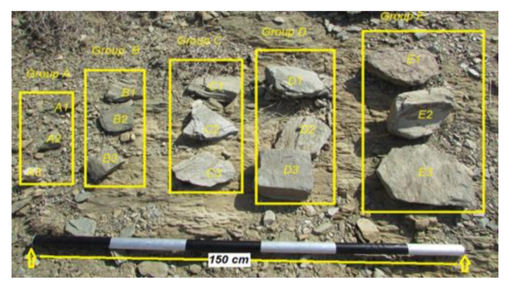
5.3. Detection Model Results

This section illustrates the experimental results of the proposed detection model. First, the eastern mountains of the Aqbat-Sha’ar were chosen as a test site to verify the model’s ability to detect the falling rocks and to track rock movement. Then, the platform was installed at a distance of twenty meters away from the mountain. Next, the test was carried out during two time periods, morning and evening. A set of fifteen differently sized rocks were used as test materials to evaluate the proposed model performance. Figure 11 presents images of test rocks divided into five groups (A, B, C, D, E), each group containing three rocks of similar sizes and a unique code.

Column four of

Table 3. System response in the morning (06:00 to 12:00).

Rock Code	Rock Size cm3	Detect Object	Disappearance Frequency N	Traceability
A1	24.53	0	0	0.0000
A2	37.06	1	21	0.9475
A3	49.00	1	15	0.9625
B1	160.93	1	14	0.9650
B2	196.25	1	12	0.9700
B3	184.00	1	12	0.9700
C1	382.68	1	10	0.9750
C2	508.32	1	7	0.9825
C3	657.04	1	6	0.9850
D1	1052.97	1	5	0.9875
D2	1012.00	1	5	0.9875
D3	1235.05	1	4	0.9900
E1	1880.49	1	3	0.9925
E2	2297.01	1	3	0.9925
E3	3041.87	1	2	0.9950

Rock code = describes a unique rock, 1 = rock is detected, 0 = no rock detected.

and

Table 4. System response in the evening (13:00 to 18:30).

Rock Code	Rock Size cm3	Detect Object	Disappearance Frequency N	Traceability
A1	24.53	0	--	0.0000
A2	37.06	0	--	0.0000
A3	49.00	0	--	0.0000
B1	160.93	1	22	0.9450
B2	196.25	1	20	0.9500
B3	184.00	1	20	0.9500
C1	382.68	1	16	0.9600
C2	508.32	1	14	0.9650
C3	657.04	1	13	0.9675
D1	1052.97	1	11	0.9725
D2	1012.00	1	11	0.9725
D3	1235.05	1	11	0.9725
E1	1880.49	1	9	0.9775
E2	2297.01	1	7	0.9825
E3	3041.87	1	6	0.9850

1 = rock detected, 0 = rock undetected, -- = unknown values.

contain the disappearance frequency N, the number of pixels in which the rock contour center disappeared from video frames until the fall reached the ground.

Column four of Table 3 and

Table 5. Simulation setups.

Parameter	Value
Driver reaction time	0.4 to 2 s
Brake Engagement time	2 s
Average acceleration	10 m/s2
Average vehicle lengths	5.4 m
Average number of vehicles driving on the road every day (NV)	6245 vehicles

contains the traceability values, assessing the model’s ability to track objects. It depends on disappearance frequency, as described in Equation (13).

$$\mathrm{Traceability}=1-\frac{\mathrm{Disappearance} \mathrm{Frequncy}}{\mathrm{Field} \mathrm{of} \mathrm{view} \mathrm{height} \mathrm{in} \mathrm{pixels}}$$

(13)

During the testing process, fifteen differently sized rocks were used. The rocks were dropped separately from a height of 22 m, and the results of the system’s response are recorded in Table 5.

The system’s ability to detect objects was evaluated by two values, zero or one—zero in the case where no event occurs and one in the case of an event occurring in the field of view. Column three of Table 5 contains the results of the objects’ detection. The result shows that the system was able to detect 93.3% of the objects in the morning and 80% in the evening.

When traceability had a value between zero and one, and field of view height represented the image frame height measured in pixels, the results showed that the average traceability in the morning at high light conditions was 0.91, while its average values during the low light conditions were 0.77. When comparing the results in Table 3 with their counterparts in Table 4, we observed that tracking rocks during the morning was better than during the evening. It was confirmed that the system’s ability to detect and track rocks during the high light is better than it is during low light conditions.

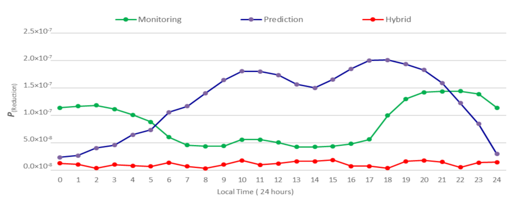
5.4. Hybrid Risk Reduction Model Results

After data were collected from the historical data of the rock-fall accidents and the traffic flow data set, we used a Python environment to simulate the rock-fall risk reduction. The hybrid model obtained it and compared the result with the obtained reduction using the detection and the prediction models separately. The configurations and the setups used for simulation are shown in Table 5.

The simulation results in Figure 12 show the effect of using the three models, monitoring, prediction, and hybrid models, separately to reduce the risk. We found that the risk probability varied from 4.26 × 10⁻⁸ to 1.44 × 10⁻⁷ with an average value of 8.62 × 10⁻⁸. When using the prediction model only, the result was represented by the blue curve. Then, when using the monitoring model only, the result was represented by the green curve. We found that the risk probability varied from 2.35 × 10⁻⁸ to 2.01 × 10⁻⁷ with an average value of 1.27 × 10⁻⁷. Finally, when using a hybrid model only, the result was represented by the red curve. We found that the risk probability varied from 3.38 × 10⁻⁹ to 1.88 × 10⁻⁸ with an average value of 1.13 × 10⁻⁸.

Table 6. Summary of risk probability after reduction.

Monitoring		Prediction	Hybrid
Lowest	4.26 × 10−8	2.35 × 10−8	3.38 × 10−9
Highest	1.44 × 10−7	2.01 × 10−7	1.88 × 10−8
Average	8.62 × 10−8	1.27 × 10−7	1.13 × 10−8

summarizes the highest and the lowest risk probabilities after reduction for the three models in addition to the average risk for each model.

By comparing the risk curves of the three models, we found that, in the case of the monitoring model, the risk probability was low between 06:00 and 18:00 and high before and after this period due to the camera’s response to sunlight and the device’s lighting at night. In a prediction model, the risk probability was high between 0:700 and 21:00 and low before and after this period due to the traffic density on the road during this period. In a hybrid model, the risk probability curve was semi-linear due to the increase in model reliability, which was gained from a parallel combination of the detection and the prediction models’ reliabilities, as mentioned in Equation (6).

In another way, the model acquired the linearity from the result of mutual compensation by the detection and the adjustment models for each other’s shortcomings. For the monitoring model, it reported an absent event as present or reported the occurrence event as absent. The prediction model corrected this situation by confirming occurrence or no occurrence of the event at this moment. In the same way, the monitoring model corrected the confusing cases of a prediction model by confirming occurrence or no occurrence of the event at this moment.

By comparing the measured risk probability after reduction, as in Table 6, with the triangle of ALARP thresholds in Figure 12, we found that the risk values were situated in an area that was usually acceptable.

5.5. Model Validation

This section summarizes the findings of system models validation. The proposed system was validated using four performance measures: sensitivity, specificity, accuracy, and reliability.

First, the prediction model’s overall prediction performance measures based on a confusion matrix (see

Table 7. Confusion matrix.

Data Type	Observed Rock-Fall Even	Predicted Rock-Fall Even		Percentage C
		Not occur 0	Occurs 1
Training Data	Not occur 0	TN = 69	FP = 11	86.3%
	Occurs 1	FN = 16	TP = 38	70.4%
	Overall Percentage			79.9%
Validation data	Not occur 0	TN = 32	FP = 5	86.5%
	Occurs 1	FN = 6	TP = 15	71.4%
	Overall Percentage			81.0%

) were evaluated for training and validation data sets. The confusion matrix was created for both training and testing. The confusion matrix was used to calculate sensitivity, specificity, and accuracy.

In the above table, true positive (TP) means all events were true detected, false negative (FN) means some events occurred but were not detected, true negative (TN) means events were absent and the system reported an absent event, and false positive (FP) means an event was absent but the system reported it as present.

The result shows that the average sensitivities of training and validation data were 70.4% and 71.4%, respectively. That means, even for the lowest sensitivity levels, only 29.6% of the rock-fall events were not detected correctly. The average specificities were about 86.3% and 86.5%, respectively, which means the system had a high ability to disregard fake events. The accuracies were 79.9% and 81.0% for the training and the validation data.

The reliability was 0.79. Next, the monitoring model performance measures were obtained by testing the system 180 times with a rock with the of size 78 cm³. The tests were divided into nine periods, and 20 tests were assigned for each period. In each period, sensitivity, specificity, and accuracy were calculated.

Table 8. System performance measures (sensitivity, specificity, accuracy).

Test Period	TP FN	FP N		Sensitivity %	Specificity %	Accuracy %
1	19 1	3	17	95	85	90
2	18 2	1	19	90	95	92.5
3	17 3	3	17	85	85	85
4	19 1	1	19	95	95	95
5	18 2	0	20	90	100	95
6	16 4	1	19	90	95	87.5
7	17 3	0	20	80	100	92.5
8	18 2	3	17	90	85	87.5
9	18 2	2	18	90	90	90

illustrates the results for all test cases.

Table 8 illustrates that the average sensitivity of the proposed method was about 88.8%, which means that, even for the lowest levels of sensitivity, only 1.2% of the rock-fall events were not detected correctly. This indicates that the system had a high sensitivity in detecting and tracking rocks. The average specificity of the proposed method was about 92.2%, which means the system had a high ability to distinguish between real and fake events. The average accuracy was 90.6. In this work, reliability was calculated according to accuracy values from Table 8, and, by using Equation (11), we obtained the system reliability equal to 0.9. That means the system had high reliability in detecting and tracking rocks and indicates that the system was valid.

Finally, the hybrid model performance measures were obtained based on its sub-models’ effects (prediction model and monitoring model). The result shows that the average sensitivity was 96.7%. That means, even for the lowest sensitivity levels, only 3.3% of the rock-fall events were not detected correctly. The proposed method’s average specificity was 99.1%, which means the system had a high ability to disregard fake events. The accuracy of 97.9% and a reliability of 0.98 indicate the goodness and the stability of the hybrid model. In another way, the model indicates high consistency.

By using the proposed hybrid model, the average risk probability was reduced from 6373 × 10⁻⁴ to 1.13 × 10⁻⁸. When comparing the hybrid model results to the monitoring and the prediction models, it must be pointed out that the proposed model outperformed the existing models. In addition, by comparing overall performance measures models, we found that the hybrid system outperformed detection and prediction models in all performance metrics, as in

Table 9. Overall models performance measures.

	Monitoring	Prediction	Hybrid
Sensitivity	71.4%	88.8%	96.7%
Specificity	86.3%	92.2%	99.1%
Accuracy	81.0%	90.6	97.9%
Reliability	0.79	0.9	0.98

.

The proposed hybrid model solved the locality problem of the prediction model through the fusion of real time weather data and detection of rock-fall events. As a result, the hybrid model can work in various locations of rock-fall. Therefore, this model can be used in reducing the rock-fall risk globally for any site. It can also be used as a road site unit in intelligent transportation systems in urban areas.

6. Conclusions and Future Work

This study aimed to develop an early warning system in the Kingdom of Saudi Arabia to minimize rock-fall risk along mountain roads. The HEWS system can predict the occurrence of a rock-fall and assess its risk probability, classifying the risk into three levels (unacceptable, tolerable, and acceptable) and delivering a proportional warning action through generating a light alarm signal (red, yellow, and green). This system was developed to overcome the limitations of our previous study (32) by increasing the system prediction reliability by combining detection and prediction models in a hybrid reliable early warning system.

In order to determine the system’s performance, this study adopted parameters, namely overall prediction performance measures, based on a confusion matrix. The results show that the overall system accuracy was 97.9%, and the hybrid model reliability was 0.98, while the previous study’s reliability was 0.90. In addition, a system can reduce the risk probability from 6.39 × 10⁻³ to 1.13 × 10⁻⁸. The result indicates that this system is accurate, reliable, and robust, confirming the utility of the proposed system for reducing rock-fall risk.

Some limitations still exist in this study. One limitation in the detection model is that it is sensitive to light intensity, causing it to fail to detect and track falling rocks smaller than 49 cm3 under low light conditions. Therefore, further work is required to enhance the detection model by increasing the night lighting intensity on the site and performing an effective frame manipulation before the background subtraction. Furthermore, the proposed method is imperfect in determining the exact moment of the rock-falls, thus future efforts should consider the short-term prediction of rock-fall events. Further work is required to enhance the predictive model by increasing the number of inventory datasets in addition to replacing the current prediction model with a new higher accuracy machine learning model.

References

1. Zhou, Z.; Lei, W.; Wu, P.; Li, B.; Fang, Y. A New Efficient Algorithm for Hazardous Material Transportation Problem via Lane Reservation. IEEE Access 2019, 7, 175290–175301. [Google Scholar] [CrossRef]
2. Youssef, A.M.; Maerz, N.H. Overview of some geological hazards in the Saudi Arabia. Environ. Earth Sci. 2013, 70, 3115–3130. [Google Scholar] [CrossRef]
3. Maerz, N.H.; Youssef, A.M.; Pradhan, B.; Bulkhi, A. Remediation and mitigation strategies for rock fall hazards along the highways of Fayfa Mountain, Jazan Region, Kingdom of Saudi Arabia. Arab. J. Geosci. 2015, 8, 2633–2651. [Google Scholar] [CrossRef]
4. Bourrier, F.; Dorren, L.; Nicot, F.; Berger, F.; Darve, F. Toward objective rockfall trajectory simulation using a stochastic impact model. Geomorphology 2009, 110, 68–79. [Google Scholar] [CrossRef] [Green Version]
5. Azzoni, A.; La Barbera, G.; Zaninetti, A. Analysis and prediction of rockfalls using a mathematical model. Int. J. Rock Mech. Min. Sci. Geomech. Abstr. 1995, 32, 709–724. [Google Scholar] [CrossRef]
6. Bunce, C.; Cruden, D.; Morgenstern, N. Assessment of the hazard from rock fall on a highway: Reply. Can. Geotech. J. 1998, 35, 410. [Google Scholar] [CrossRef]
7. Katz, O.; Reichenbach, P.; Guzzetti, F. Rock fall hazard along the railway corridor to Jerusalem, Israel, in the Soreq and Refaim valleys. Nat. Hazards 2011, 56, 649–665. [Google Scholar] [CrossRef]
8. Asteriou, P.; Tsiambaos, G. Effect of impact velocity, block mass and hardness on the coefficients of restitution for rockfall analysis. Int. J. Rock Mech. Min. Sci. 2018, 106, 41–50. [Google Scholar] [CrossRef]
9. Dadashzadeh, N.; Duzgun, H.; Yesiloglu-Gultekin, N. Reliability-based stability analysis of rock slopes using numerical analysis and response surface method. Rock Mech. Rock Eng. 2017, 50, 2119–2133. [Google Scholar] [CrossRef]
10. Ersöz, T.; Topal, T. Assessment of rock slope stability with the effects of weathering and excavation by comparing deterministic methods and slope stability probability classification (SSPC). Environ. Earth Sci. 2018, 77, 547. [Google Scholar] [CrossRef]
11. Sharma, P.; Verma, A.K.; Negi, A.; Jha, M.K.; Gautam, P. Stability assessment of jointed rock slope with different crack infillings under various thermomechanical loadings. Arab. J. Geosci. 2018, 11, 431. [Google Scholar] [CrossRef]
12. Shen, W.; Zhao, T.; Dai, F.; Zhou, J.; Xu, N. Investigation of Rockfall Impact Against Gravel Cushion via a Discrete Element Approach. In Proceedings of the China-Europe Conference on Geotechnical Engineering, Cham, Switzerland, 13–16 August 2018; pp. 1521–1525. [Google Scholar]
13. Budetta, P. Assessment of rockfall risk along roads. Nat. Hazards Earth Syst. Sci. 2004, 4, 71–81. [Google Scholar] [CrossRef] [Green Version]
14. Luciano, P. Quantitative risk assessment of rockfall hazard in the amalfi coastal road. Available online: https://upcommons.upc.edu/handle/2099.1/4937 (accessed on 1 February 2021).
15. Sun, S.-Q.; Li, L.-P.; Li, S.-C.; Zhang, Q.-Q.; Hu, C. Rockfall Hazard Assessment on Wangxia Rock Mass in Wushan (Chongqing, China). Geotech. Geol. Eng. 2017, 35, 1895–1905. [Google Scholar] [CrossRef]
16. Paronuzzi, P. Rockfall-induced block propagation on a soil slope, northern Italy. Environ. Geol. 2009, 58, 1451–1466. [Google Scholar] [CrossRef]
17. Chen, G.; Zheng, L.; Zhang, Y.; Wu, J. Numerical Simulation in Rockfall Analysis: A Close Comparison of 2-D and 3-D DDA. Rock Mech. Rock Eng. 2013, 46, 527–541. [Google Scholar] [CrossRef]
18. Li, L.; Lan, H. Probabilistic modeling of rockfall trajectories: A review. Bull. Int. Assoc. Eng. Geol. 2015, 74, 1163–1176. [Google Scholar] [CrossRef]
19. Steiakakis, C.; Partsinevelos, P.; Tripolitsiotis, A.; Agioutantis, Z; Mertikas, S.; Vlahou, G. Design and System Architecture of the GEOIM Rockfall Monitoring System. In 5th Interdisciplinary Workshop on Rockfall Protection-RocExs; RocExs: Lecco, Italy, 2014. [Google Scholar]
20. Collins, D.S.; Toya, Y.; Hosseini, Z.; Trifu, C.I. Real Time Detection of Rock Fall Events Using a Microseismic Railway Monitoring System; Geohazards: Kingstone, ON, Canada, 2014. [Google Scholar]
21. Gracchi, T.; Lotti, A.; Saccorotti, G.; Lombardi, L.; Nocentini, M.; Mugnai, F.; Gigli, G.; Barla, M.; Giorgetti, A.; Antolini, F. A method for locating rockfall impacts using signals recorded by a microseismic network. Geoenviron. Disasters 2017, 4, 26. [Google Scholar] [CrossRef]
22. Pieš, M.; Hájovský, R. Use of accelerometer sensors to measure the states of retaining steel networks and dynamic barriers. In Proceedings of the 2018 19th International Carpathian Control Conference (ICCC), Szilvasvarad, Hungary, 28–31 May 2018; pp. 416–421. [Google Scholar]
23. Caviezel, A.; Schaffner, M.; Cavigelli, L.; Niklaus, P.; Buhler, Y.; Bartelt, P.; Magno, M.; Benini, L. Design and Evaluation of a Low-Power Sensor Device for Induced Rockfall Experiments. IEEE Trans. Instrum. Meas. 2017, 67, 767–779. [Google Scholar] [CrossRef] [Green Version]
24. Lato, M.; Hutchinson, J.; Diederichs, M.; Ball, D.; Harrap, R. Engineering monitoring of rockfall hazards along transportation corridors: Using mobile terrestrial LiDAR. Nat. Hazards Earth Syst. Sci. 2009, 9, 935–946. [Google Scholar] [CrossRef]
25. Hartmeyer, I.; Keuschnig, M.; Schrott, L. Implementing a long-term monitoring site focusing on permafrost and rockfall interaction at the Kitzsteinhorn (3.203 m), Hohe Tauern Range, Austria–A status report from the MOREXPERT project. In Conference Volume of the 5th Symposium for Research in Protected Areas; Sekretariat des Nationalparkrates Hohe Tauern: Osttirol, Austria, 2013; Volume 2. [Google Scholar]
26. Tonini, M.; Abellán, A. Rockfall detection from terrestrial LiDAR point clouds: A clustering approach using R. J. Spat. Inf. Sci. 2014, 8, 95–110. [Google Scholar] [CrossRef]
27. van Veen, M.; Hutchinson, D. J.; Kromer, R.; Lato, M.; Edwards, T. Effects of sampling interval on the frequency-magnitude relationship of rockfalls detected from terrestrial laser scanning using semi-automated methods. Landslides 2017, 14, 1579–1592. [Google Scholar] [CrossRef]
28. Gigli, G.; Morelli, S.; Fornera, S.; Casagli, N. TXT-tool 4.039-3.1: Terrestrial Laser Scanner and Geomechanical Surveys for the Rapid Evaluation of Rock Fall Susceptibility Scenarios. In Landslide Dynamics: ISDR-ICL Landslide Interactive Teaching Tools; Springer: Cham, Switzerland, 2018; pp. 477–491. [Google Scholar]
29. Fantini, A.; Fiorucci, M.; Martino, S. Rock falls impacting railway tracks: Detection analysis through an artificial intelligence camera prototype. Wirel. Commun. Mob. Comput. 2017, 2017, 9386928. [Google Scholar] [CrossRef] [Green Version]
30. Shirzadi, A.; Saro, L.; Joo, O.H.; Chapi, K. A GIS-based logistic regression model in rock-fall susceptibility mapping along a mountainous road: Salavat Abad case study, Kurdistan, Iran. Nat. Hazards 2012, 64, 1639–1656. [Google Scholar] [CrossRef] [Green Version]
31. Frattini, P.; Crosta, G.; Carrara, A.; Agliardi, F. Assessment of rockfall susceptibility by integrating statistical and physically-based approaches. Geomorphology 2008, 94, 419–437. [Google Scholar] [CrossRef]
32. Abaker, M.; Abdelmaboud, A.; Osman, M.; Alghobiri, M.; Abdelmotlab, A. A Rock-fall Early Warning System Based on Logistic Regression Model. Intell. Autom. Soft Comput. 2021, 28, 843–856. [Google Scholar] [CrossRef]
33. Aoun, A.G. Aqabats Shaar and Dele Two Obstacles in the Life Test. 2010. Available online: https://www.okaz.com.sa/article/365122 (accessed on 11 January 2021).
34. Al-Andijani, T. The Geological Survey Completes the Study of Rockfalls in Aqabat Shaar in the Asir Region. 2005. Available online: https://www.alriyadh.com/82375 (accessed on 17 January 2021).
35. Was. Rockslides Cause the Hurdles of Shaar and Dhula to Be Closed, and “Asir Transport” Begins Their Maintenance. 2020. Available online: https://www.spa.gov.sa/2117551 (accessed on 19 February 2021).
36. Delonca, A.; Gunzburger, Y.; Verdel, T. Statistical correlation between meteorological and rockfall databases. Nat. Hazards Earth Syst. Sci. 2014, 14, 1953–1964. [Google Scholar] [CrossRef] [Green Version]
37. D’Amato, J.; Hantz, D.; Guerin, A.; Jaboyedoff, M.; Baillet, L.; Mariscal, A. Influence of meteorological factors on rockfall occurrence in a middle mountain limestone cliff. Nat. Hazards Earth Syst. Sci. 2016, 16, 719–735. [Google Scholar] [CrossRef] [Green Version]
38. Berti, M.; Martina, M.L.V.; Franceschini, S.; Pignone, S.; Simoni, A.; Pizziolo, M. Probabilistic rainfall thresholds for landslide occurrence using a Bayesian approach. J. Geophys. Res. Space Phys. 2012, 117, F4. [Google Scholar] [CrossRef] [Green Version]
39. Collins, B.D.; Stock, G.M. Rockfall triggering by cyclic thermal stressing of exfoliation fractures. Nat. Geosci. 2016, 9, 395–400. [Google Scholar] [CrossRef]
40. Shirzadi, A.; Chapi, K.; Shahabi, H.; Solaimani, K.; Kavian, A.; Bin Ahmad, B. Rock fall susceptibility assessment along a mountainous road: An evaluation of bivariate statistic, analytical hierarchy process and frequency ratio. Environ. Earth Sci. 2017, 76, 152. [Google Scholar] [CrossRef]
41. Scavia, C.; Barbero, M.; Castelli, M.; Marchelli, M.; Peila, D.; Torsello, G.; Vallero, G. Evaluating Rockfall Risk: Some Critical Aspects. Geosciences 2020, 10, 98. [Google Scholar] [CrossRef] [Green Version]
42. Kaewfak, K.; Huynh, V.-N.; Ammarapala, V.; Ratisoontorn, N. A Risk Analysis Based on a Two-Stage Model of Fuzzy AHP-DEA for Multimodal Freight Transportation Systems. IEEE Access 2020, 8, 153756–153773. [Google Scholar] [CrossRef]
43. Wang, X.; Frattini, P.; Crosta, G.B.; Zhang, L.; Agliardi, F.; Lari, S.; Yang, Z. Uncertainty assessment in quantitative rockfall risk assessment. Landslides 2013, 11, 711–722. [Google Scholar] [CrossRef]
44. Lee, S. Application of logistic regression model and its validation for landslide susceptibility mapping using GIS and remote sensing data. Int. J. Remote Sens. 2005, 26, 1477–1491. [Google Scholar] [CrossRef]
45. Tian, G.; Liu, Y.; Tang, M. Logistic regression analysis of non-randomized response data collected by the parallel model in sensitive surveys. Aust. N. Z. J. Stat. 2019, 61, 134–151. [Google Scholar] [CrossRef]
46. Huang, S.; Lyu, Y.; Peng, Y.; Huang, M. Analysis of Factors Influencing Rockfall Runout Distance and Prediction Model Based on an Improved KNN Algorithm. IEEE Access 2019, 7, 66739–66752. [Google Scholar] [CrossRef]
47. Wang, X.-T.; Li, S.-C.; Ma, X.-Y.; Xue, Y.-G.; Hu, J.; Li, Z.-Q. Risk Assessment of Rockfall Hazards in a Tunnel Portal Section Based on Normal Cloud Model. Pol. J. Environ. Stud. 2017, 26, 2295–2306. [Google Scholar] [CrossRef]
48. Kromer, R.; Lato, M.; Hutchinson, D.J.; Gauthier, D.; Edwards, T. Managing rockfall risk through baseline monitoring of precursors using a terrestrial laser scanner. Can. Geotech. J. 2017, 54, 953–967. [Google Scholar] [CrossRef]
49. Park, J.G.; Lee, C. Bayesian rule-based complex background modeling and foreground detection. Opt. Eng. 2010, 49, 027006. [Google Scholar] [CrossRef]
50. Budetta, P.; Nappi, M. Comparison between qualitative rockfall risk rating systems for a road affected by high traffic intensity. Nat. Hazards Earth Syst. Sci. 2013, 13, 1643. [Google Scholar] [CrossRef] [Green Version]
51. Gholizadeh, R.; Londono, S.L.M.; Barahona, M.J.P. Expectation Bayesian Estimation of System Reliability Based on Failures. Methodol. Comput. Appl. Probab. 2018, 21, 367–385. [Google Scholar] [CrossRef]
52. Szydłowski, T.; Surmiński, K.; Batory, D. Drivers’ Psychomotor Reaction Times Tested with a Test Station Method. Appl. Sci. 2021, 11, 2431. [Google Scholar] [CrossRef]
53. Zeng, G. On the confusion matrix in credit scoring and its analytical properties. Commun. Stat. Theory Methods 2019, 49, 2080–2093. [Google Scholar] [CrossRef]
54. Nesticò, A.; He, S.; De Mare, G.; Benintendi, R.; Maselli, G. The ALARP Principle in the Cost-Benefit Analysis for the Acceptability of Investment Risk. Sustainability 2018, 10, 4668. [Google Scholar] [CrossRef] [Green Version]
Figure 1. Examples of rockfall problems in Aqabat Shaar. (a) Effect of road construction. (b) Effect of tunnel construction. (c) Effect of floods. (d) Effect of erosion.
Applsci 11 09506 g001
Figure 2. Methodology flowchart.
Applsci 11 09506 g002
Figure 3. Detection model development steps.
Applsci 11 09506 g003
Figure 4. Field of view calibration process steps.
Applsci 11 09506 g004
Figure 5. Perspective view of a mountain in image plane (a). Perspective corrected image in world plane (b).
Applsci 11 09506 g005
Figure 6. Rock-fall detection process.
Applsci 11 09506 g006
Figure 7. Hybrid early warning system block diagram.
Applsci 11 09506 g007
Figure 8. Hybrid early warning system platform.
Applsci 11 09506 g008
Figure 9. Rock-fall risk probability.
Applsci 11 09506 g009
Figure 10. ALARP thresholds triangle.
Applsci 11 09506 g010
Figure 11. Sample rocks for testing.
Applsci 11 09506 g011
Figure 12. Rock-fall risk probability after being reduced by the system models.
Applsci 11 09506 g012