
Nonlinear Dynamic Response of Ropeway Roller Batteries via an Asymptotic Approach


Abstract
:1. Introduction
2. Nonlinear Dynamic Characterization
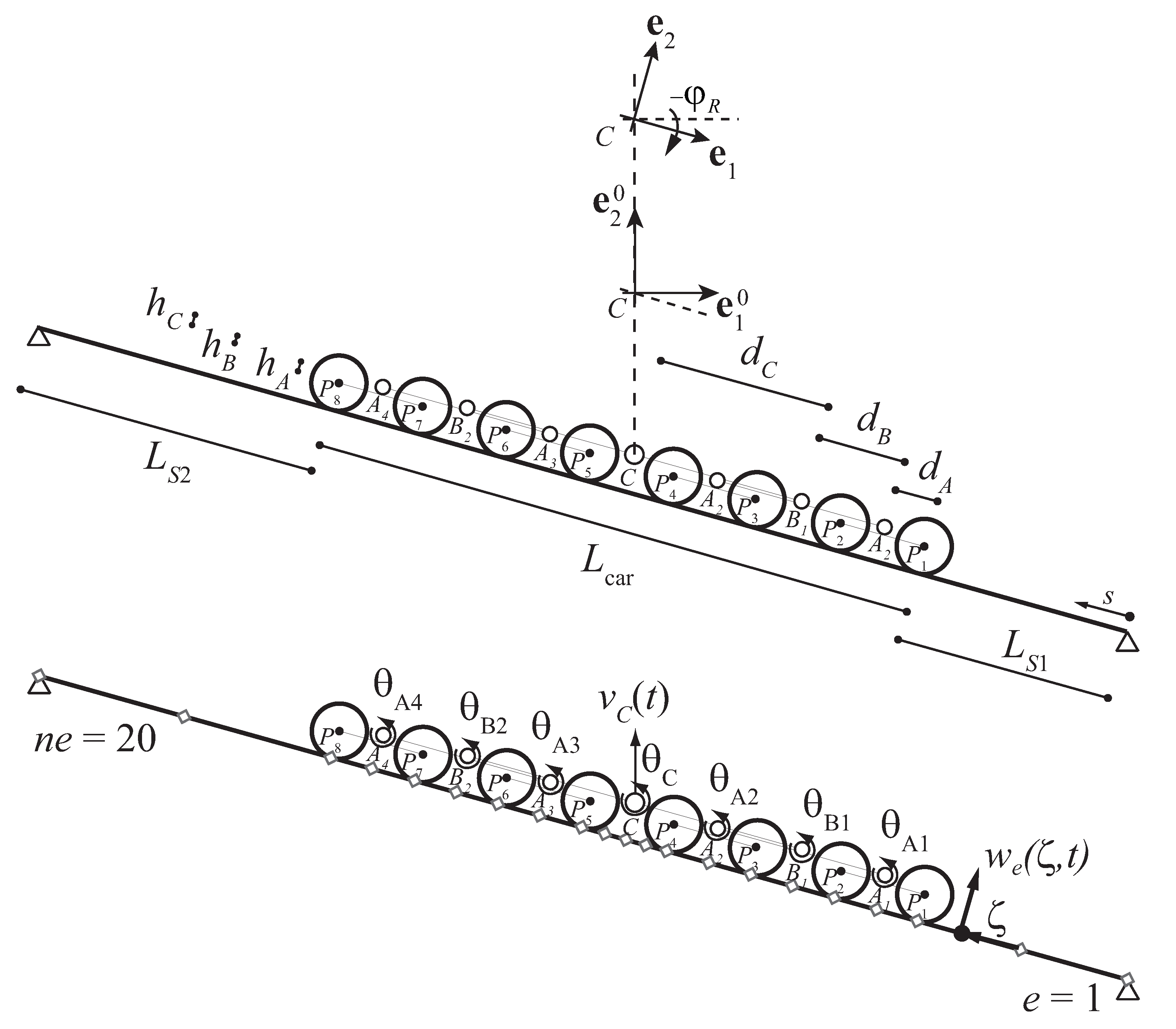
2.1. Kinematic Descriptors
2.2. Nonlinear Equations of Motion
2.3. Nondimensional Vector Form of the Equations of Motion
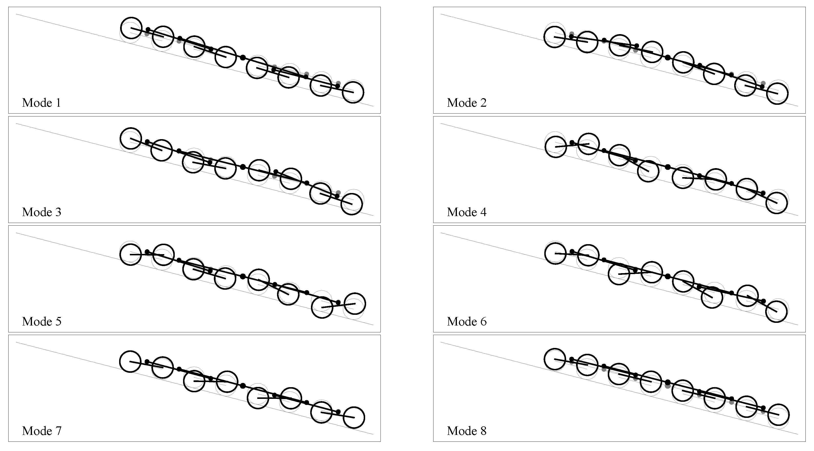
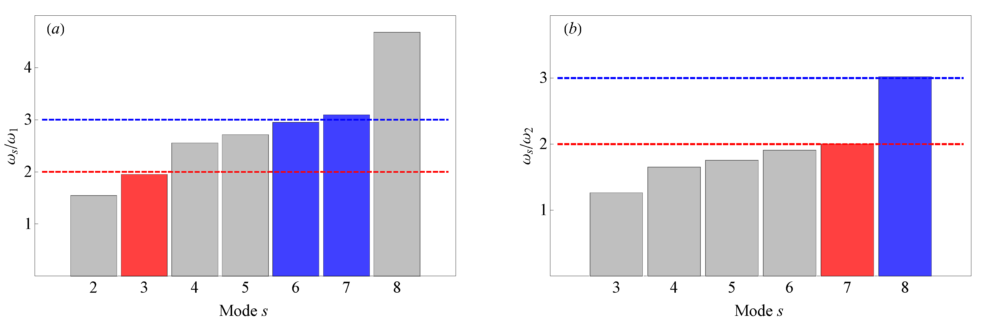
3. Modal Characterization
4. Asymptotic Solution of the Equations of Motion
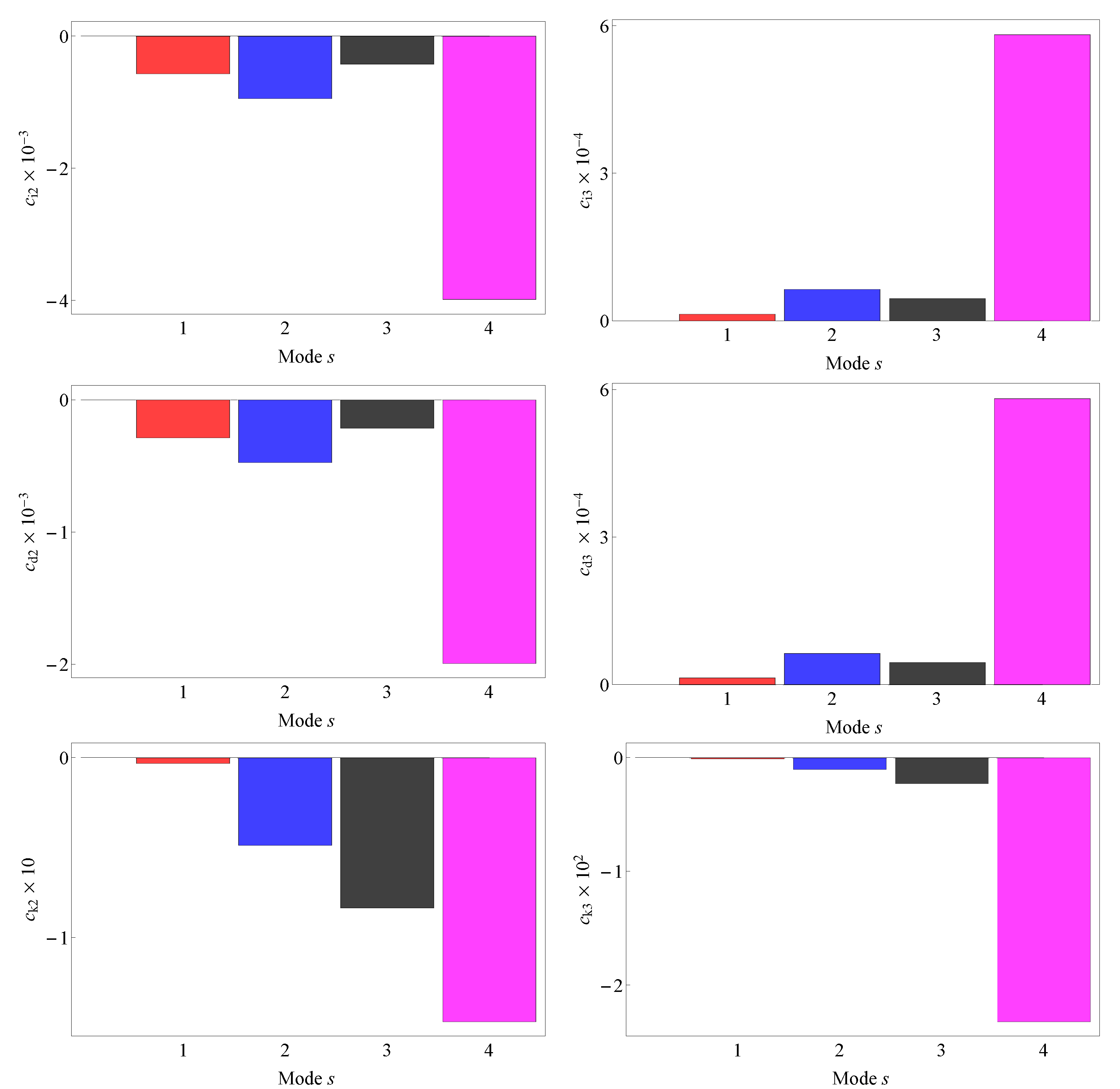
4.1. Nonlinearity of the Lowest Normal Modes
One-Mode Projection of the Nonlinear Equations of Motion
5. Cable Motion-Induced Resonances
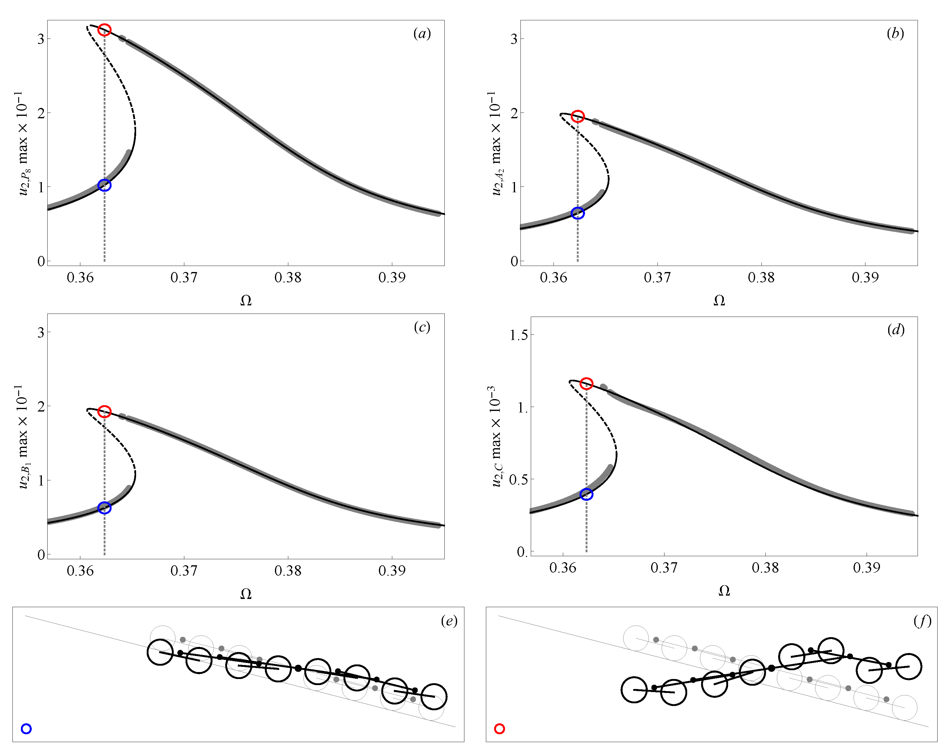
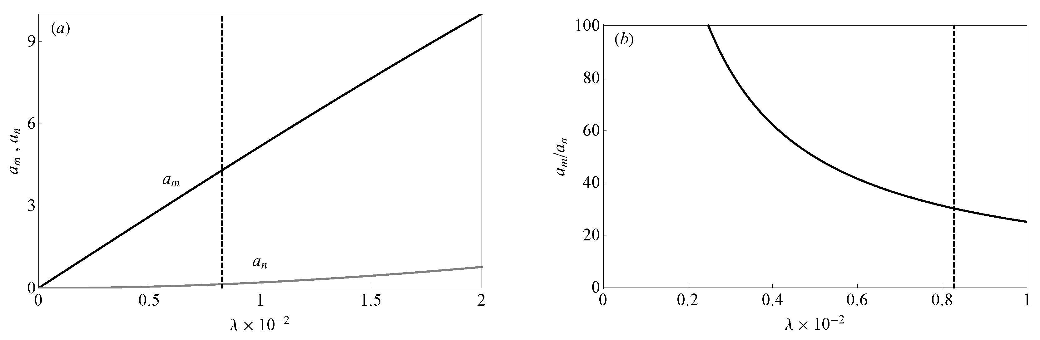
5.1. Primary Resonance
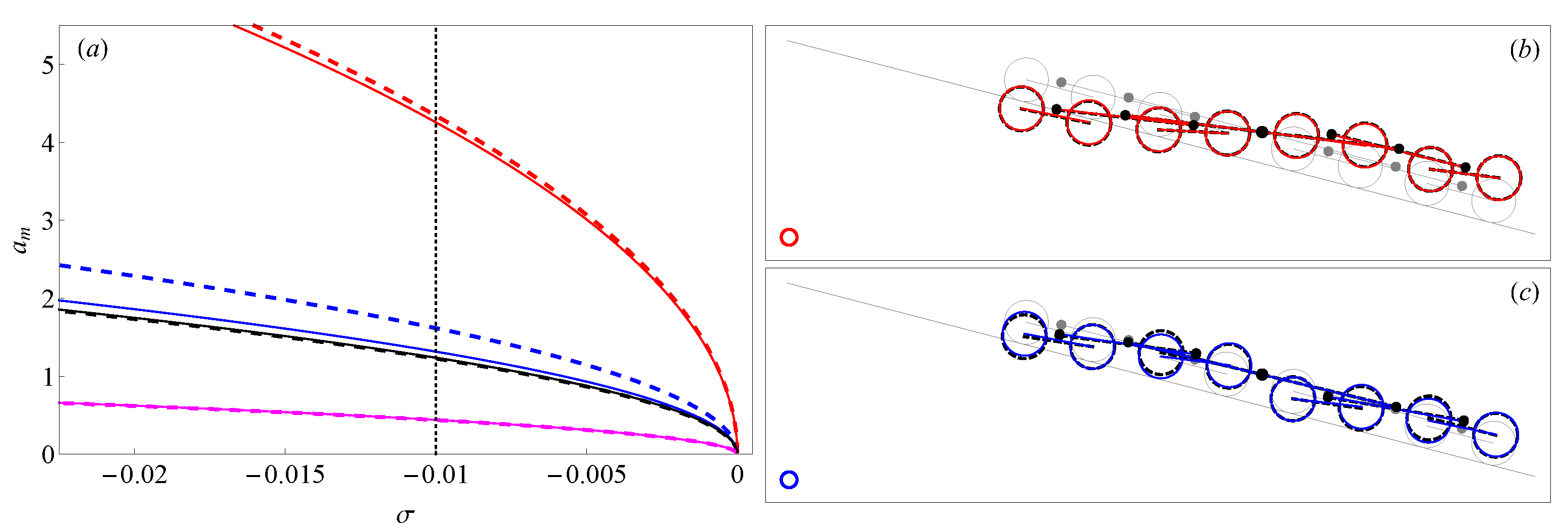
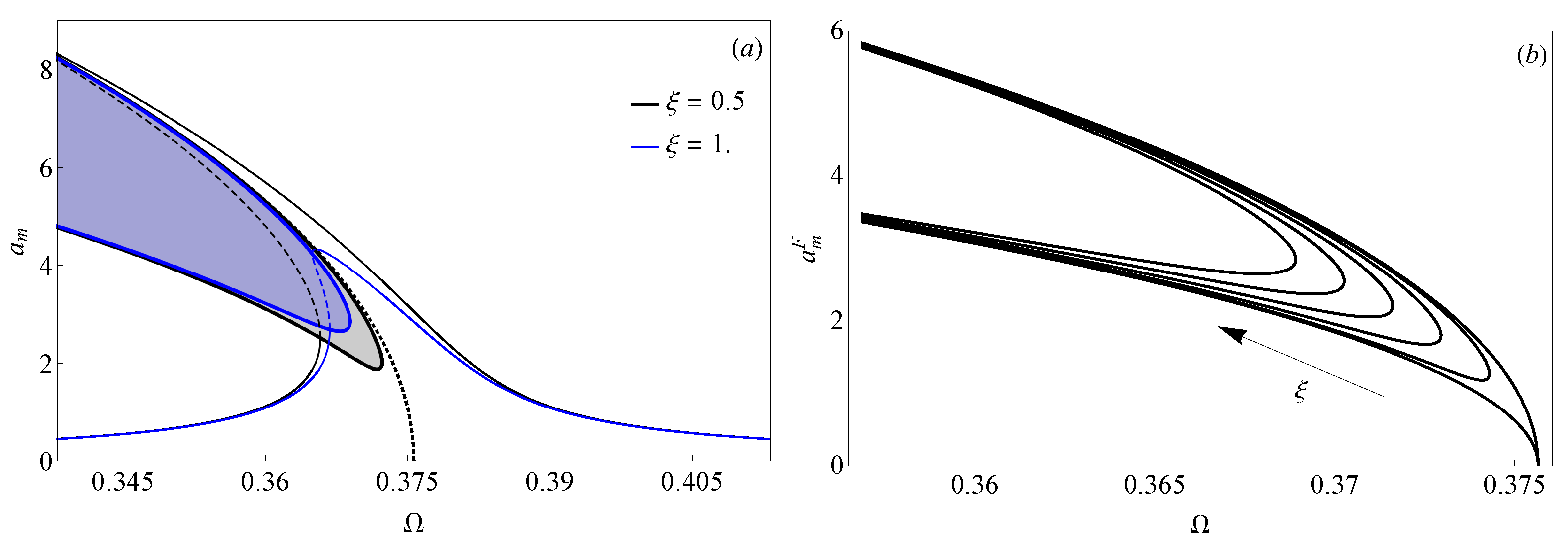
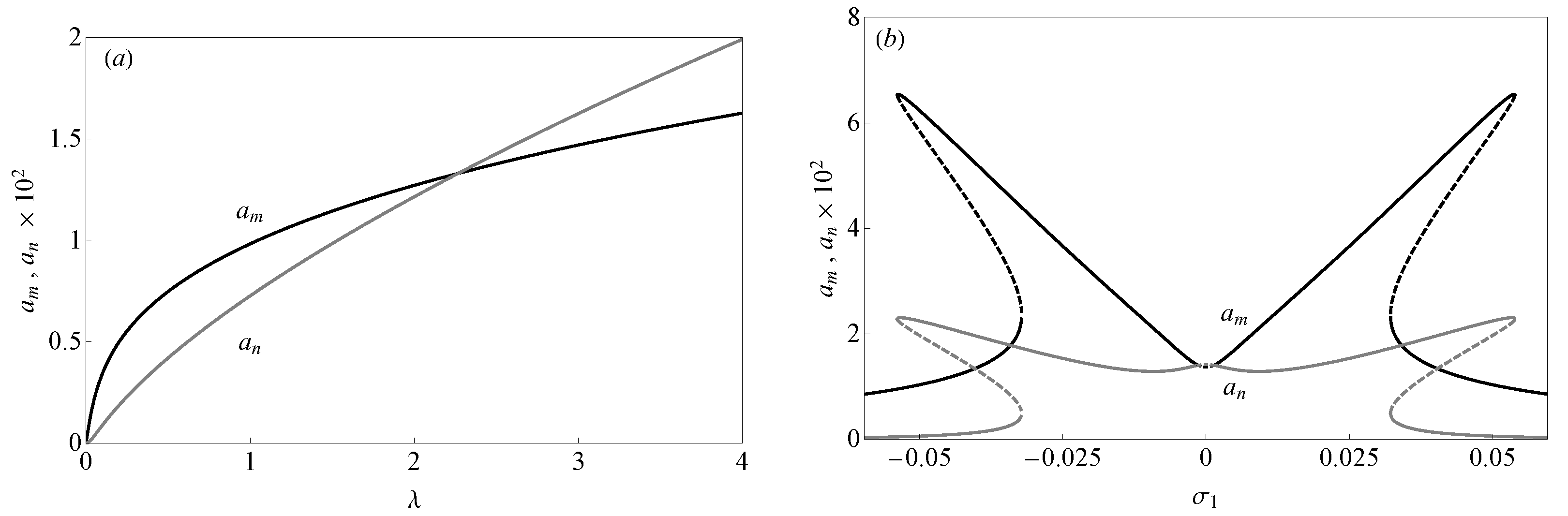
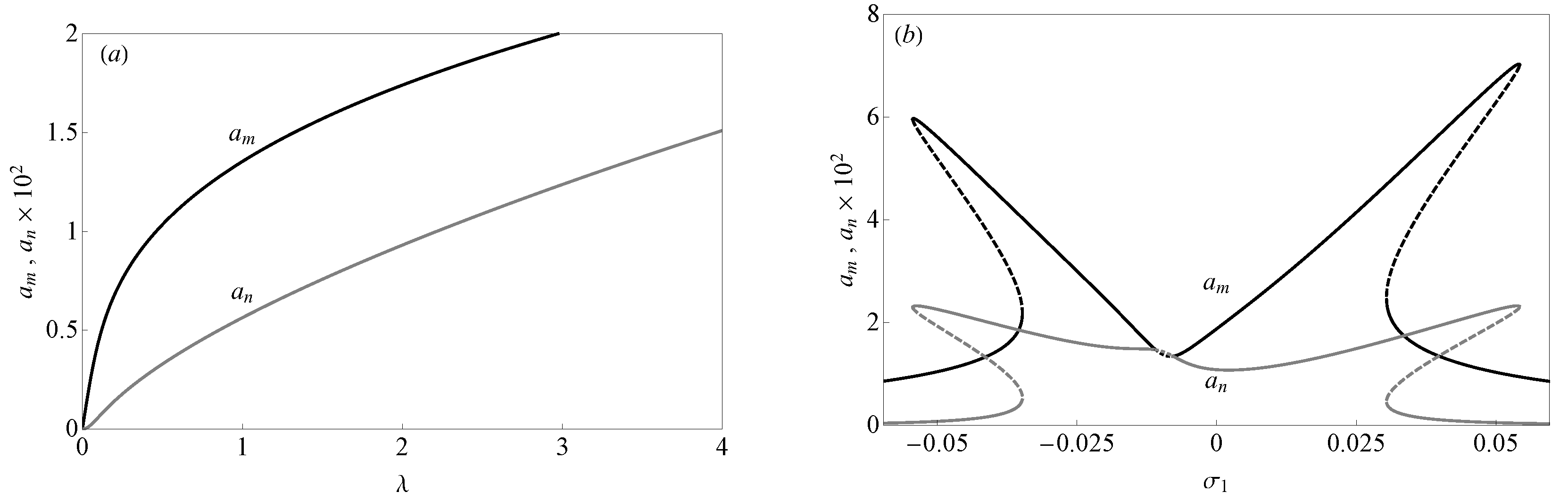
5.2. Two-to-One Internal Resonance
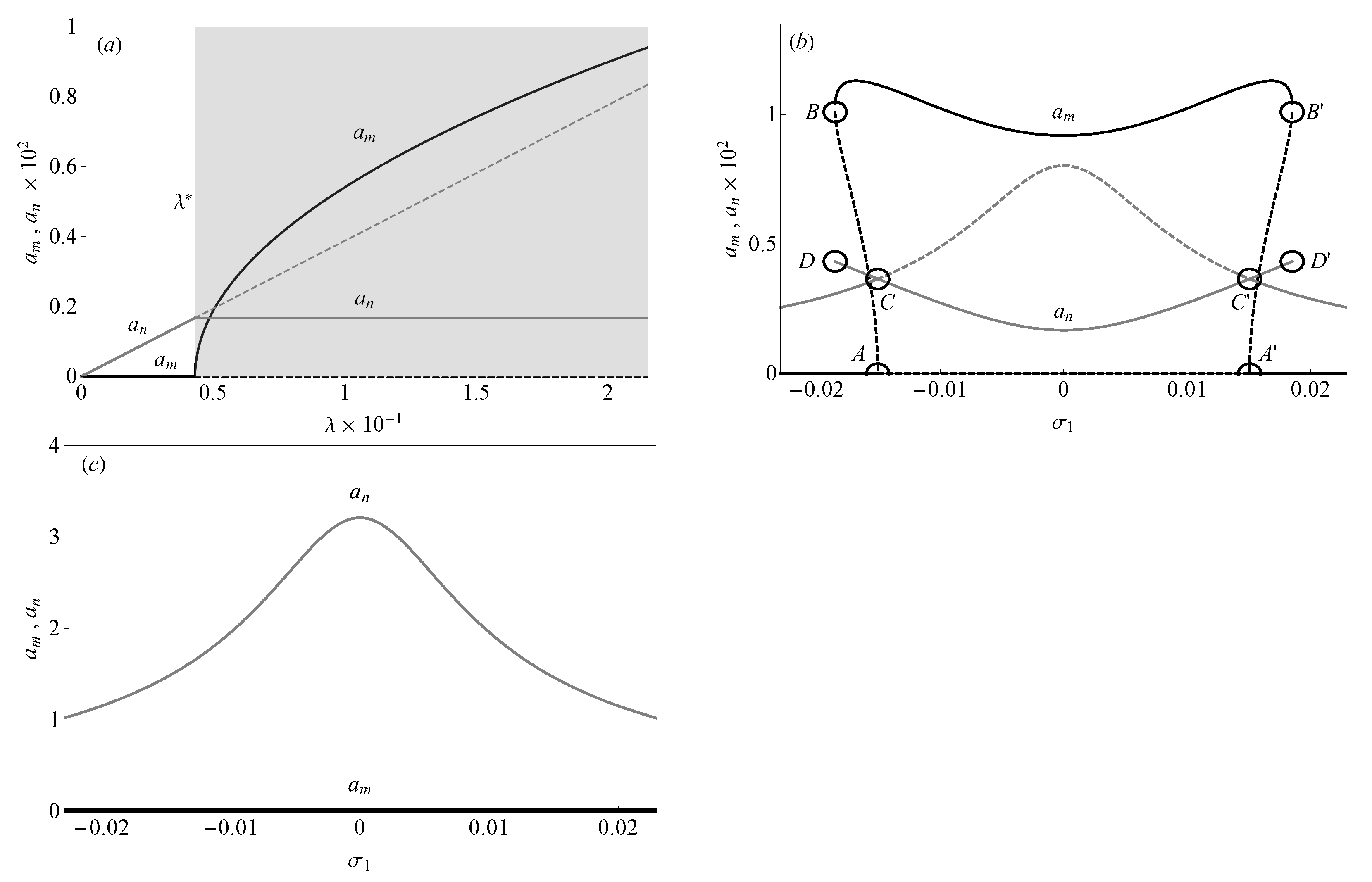
5.2.1. The Case of
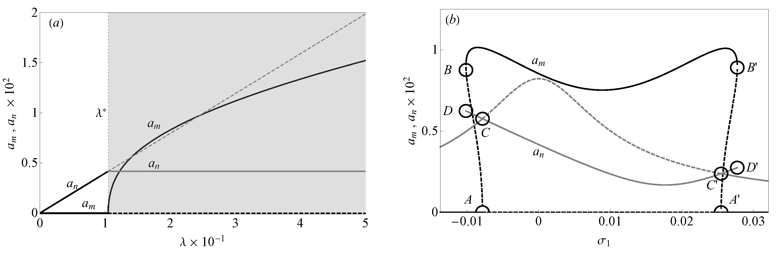
5.2.2. The Case of
6. Conclusions
Funding
Acknowledgments
Conflicts of Interest
References
- Alshalalfah, B.W.; Shalaby, A.S.; Dale, S.; Othman, F.M. Feasibility Study of Aerial Ropeway Transit in the Holy City of Makkah. Transp. Plan. Technol. 2015, 38, 392–408. [Google Scholar] [CrossRef]
- Hoffmann, K.; Liehl, R. Cable-drawn urban transport systems. WIT Trans. Built Environ. 2005, 77, 25–36. [Google Scholar]
- Hoffmann, K.; Gabmayer, T.; Huber, G. Measurement of Oscillation Effects on Ropeways and Chairlifts. ÖIAZ 2008, 153, 435–438. [Google Scholar]
- Portier, B. Dynamic Phenomena in Ropeway after a Haul Rope Rapture. Earthq. Eng. Struct. Dyn. 1984, 12, 433–449. [Google Scholar] [CrossRef]
- Brownjohn, J.W. Dynamics of Aerial Cableway System. Eng. Struct. 1998, 20, 826–836. [Google Scholar] [CrossRef]
- Renezeder, H.; Steindl, A.; Troger, H. On the Dynamics of Circulating Monocable Aerial Ropeways. Proc. Appl. Math. Mech. 2005, 5, 123–124. [Google Scholar] [CrossRef]
- Bryja, D.; Knawa, M. Computational Model of an Inclined Aerial Ropeway and Numerical Method for Analyzing Nonlinear Cable-car Interaction. Comput. Struct. 2011, 89, 1895–1905. [Google Scholar] [CrossRef]
- Knawa-Hawryszków, M. Determining initial tension of carrying cable in nonlinear analysis of bi-cable ropeway—Case study. Eng. Struct. 2021, 244, 1–13. [Google Scholar] [CrossRef]
- Wenin, M.; Windisch, A.; Ladurner, S.; Bertotti, M.L.; Modanese, G. Optimal velocity profile for a cable car passing over a support. Eur. J. Mech./A Solids 2019, 73, 366–372. [Google Scholar] [CrossRef]
- Wenin, M.; Ladurner, S.; Reiterer, D.; Bertotti, M.L.; Modanese, G. Validation of the Velocity Optimization for a Ropeway Passingover a Support. Sustainability 2021, 13, 2986. [Google Scholar] [CrossRef]
- Nan, C.; Meyer-Piening, H.R.; Decking, C. Dynamic Behaviour of Cable Supporting Roller Batteries: Basic Model. Comput. Struct. 1998, 69, 95–104. [Google Scholar] [CrossRef]
- Arena, A.; Carboni, B.; Lacarbonara, W.; Babaz, M. Dynamic response and identification of tower-cable-roller battery interactions in ropeways. In Proceedings of the ASME Design Engineering Technical Conference, IDETC/CIE 2017, Cleveland, OH, USA, 6–9 August 2017; ASME: New York, NY, USA, 2017; Volume 6. [Google Scholar]
- Arena, A.; Carboni, B.; Lacarbonara, W.; Babaz, M. Ropeway roller batteries dynamics: Modeling, identification, and full-scalevalidation. Eng. Struct. 2019, 180, 793–808. [Google Scholar] [CrossRef]
- Carboni, B.; Arena, A.; Lacarbonara, W. Passive vibration control of roller batteries in cableways. In Proceedings of the ASME Design Engineering Technical Conference, IDETC/CIE 2018, Quebec City, QC, Canada, 26–29 August 2018; ASME: New York, NY, USA, 2018; Volume 6. [Google Scholar]
- Carboni, B.; Arena, A.; Lacarbonara, W. Nonlinear vibration absorbers for ropeway roller batteries control. Proc. Inst. Mech. Eng. Part C J. Mech. Eng. Sci. 2020, 1–15. [Google Scholar] [CrossRef]
- Abdel-Rahman, E.M.; Nayfeh, A.H.; Masoud, Z. Dynamics and control of cranes: A review. J. Vib. Control 2001, 9, 863–908. [Google Scholar] [CrossRef]
- Cartmell, M.P. On the need for control of nonlinear oscillations in machine systems. Meccanica 2003, 38, 185–212. [Google Scholar] [CrossRef]
- Ellermann, K.; Kreuzer, E.; Markiewicz, M. Nonlinear primary resonances of a floating crane. Meccanica 2003, 38, 4–17. [Google Scholar] [CrossRef]
- Arena, A.; Lacarbonara, W.; Cartmell, M.P. Nonlinear Interactions in Deformable Container Cranes. Proc IMechE Part C J. Mech. Eng. Sci. 2016, 230, 5–20. [Google Scholar] [CrossRef] [Green Version]
- Zukovic, M.; Kovacic, I.; Cartmell, M.P. On the dynamics of a parametrically excited planar tether. Commun. Nonlinear Sci. Numer. Simul. 2015, 26, 250–264. [Google Scholar] [CrossRef]
- Cartmell, M.P.; Kovacic, I.; Zukovic, M. Autoparametric interaction in a double pendulum system. Proc. Inst. Mech. Eng. Part C J. Mech. Eng. Sci. 2012, 226, 1971–1986. [Google Scholar] [CrossRef]
- Kovacic, I.; Zukovic, M.; Cartmell, M.P. On the oscillation death phenomenon in a double pendulum system with autoparametric interaction. J. Phys. Conf. Ser. 2012, 382, 012055. [Google Scholar] [CrossRef] [Green Version]
- Moura, A.G.; Erturk, A. Combined piezoelectric and flexoelectric effects in resonant dynamics of nanocantilevers. J. Intell. Mater. Syst. Struct. 2018, 24, 266–273. [Google Scholar] [CrossRef]
- Arena, A.; Lacarbonara, W. Piezoelectrically induced nonlinear resonances for dynamic morphing of lightweight panels. J. Sound Vib. 2021, 498, 115951. [Google Scholar] [CrossRef]
- Yuda, H.; Jing, L. The magneto-elastic subharmonic resonance of current-conducting thin plate in magnetic filed. J. Sound Vib. 2009, 319, 1107–1120. [Google Scholar] [CrossRef]
- Givois, A.; Giraud-Audine, C.; Deü, J.F.; Thomas, O. Experimental analysis of nonlinear resonances in piezoelectric plates with geometric nonlinearities. Nonlinear Dyn. 2020, 102, 1451–1462. [Google Scholar] [CrossRef]
- Luongo, A.; Rega, G.; Vestroni, F. On Nonlinear Dynamics of Planar Shear Indeformabie Beams. J. Appl. Mech. 1986, 53, 619–624. [Google Scholar] [CrossRef]
- Rahman, Z.; Burton, T.D. Large amplitude primary and superharmonic resonances in the duffing oscillator. J. Sound Vib. 1986, 110, 363–380. [Google Scholar] [CrossRef]
- Rahman, Z.; Burton, T.D. On higher order methods of multiple scales in non-linear oscillations-periodic steady state response. J. Sound Vib. 1989, 133, 369–379. [Google Scholar] [CrossRef]
- Wojnowsky Krieger, S. The Effect of an Axial Force on the Vibration of Hinged Bars. J. Appl. Mech. 1950, 17, 35–36. [Google Scholar] [CrossRef]
- Eisley, J.G. Nonlinear vibration of beams and rectangular plates. J. Appl. Math. Phys. (ZAMP) 1964, 15, 167–175. [Google Scholar] [CrossRef] [Green Version]
- Evensen, D.A. Nonlinear Vibrations of Beams with Various Boundary Conditions. Am. Inst. Aeronaut. Astronaut. J. 1968, 6, 370–372. [Google Scholar] [CrossRef]
- Nayfeh, A.H.; Mook, D.T.; Lobitz, D.W. Numerical-Perturbation Method for the Nonlinear Analysis of Structural Vibrations. Am. Inst. Aeronaut. Astronaut. J. 1974, 12, 1222–1228. [Google Scholar] [CrossRef]
- Nayfeh, A.H.; Mook, D.T. Nonlinear Oscillations; Wiley-Interscience: New York, NY, USA, 1979. [Google Scholar]
- Nayfeh, A.H. Introduction to Perturbation Techniques; John Wiley & Sons: Hoboken, NJ, USA, 1993. [Google Scholar]
- Nayfeh, A.H. Nonlinear Interactions: Analytical Computational and Experimental Methods; John Wiley and Sons Ltd.: New York, NY, USA, 2000. [Google Scholar]
- Wolfram Research, Inc. Mathematica, Version 11.0; Wolfram Research, Inc.: Champaign, IL, USA, 2016. [Google Scholar]

| Mode s | 1 | 2 | 3 | 4 |
| 0.376 | 0.581 | 0.734 | 0.96 | |
| Mode s | 5 | 6 | 7 | 8 |
| 1.02 | 1.109 | 1.163 | 1.757 |
| All | Inertia | Velocity | Stiffness | |
|---|---|---|---|---|
Publisher’s Note: MDPI stays neutral with regard to jurisdictional claims in published maps and institutional affiliations. |
© 2021 by the author. Licensee MDPI, Basel, Switzerland. This article is an open access article distributed under the terms and conditions of the Creative Commons Attribution (CC BY) license (https://creativecommons.org/licenses/by/4.0/).
Share and Cite
Arena, A. Nonlinear Dynamic Response of Ropeway Roller Batteries via an Asymptotic Approach. Appl. Sci. 2021, 11, 9486. https://doi.org/10.3390/app11209486
Arena A. Nonlinear Dynamic Response of Ropeway Roller Batteries via an Asymptotic Approach. Applied Sciences. 2021; 11(20):9486. https://doi.org/10.3390/app11209486
Chicago/Turabian StyleArena, Andrea. 2021. "Nonlinear Dynamic Response of Ropeway Roller Batteries via an Asymptotic Approach" Applied Sciences 11, no. 20: 9486. https://doi.org/10.3390/app11209486
APA StyleArena, A. (2021). Nonlinear Dynamic Response of Ropeway Roller Batteries via an Asymptotic Approach. Applied Sciences, 11(20), 9486. https://doi.org/10.3390/app11209486