
Fundamental Investigations on the Performance of Micro Steel Fibres in Ultra-High-Performance Concrete under Monotonic and Cyclic Tensile Loading


Abstract
:1. Introduction
2. Fibre Design Philosophy
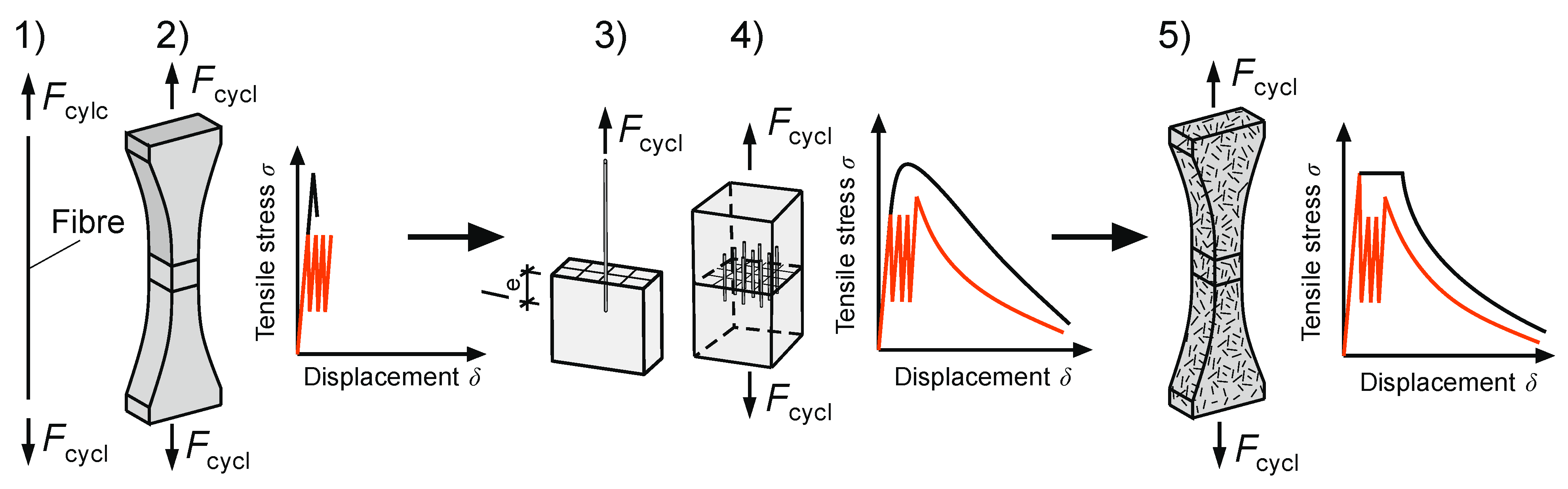
3. Investigation Strategy
- Micro steel fibre (“bare”)—part 1.
- Plain UHPC—part 2.
- UHPC–fibre interaction of single fibres and fibre groups—parts 3 and 4.
- Tensile tests on small UHPFRC samples—part 5.
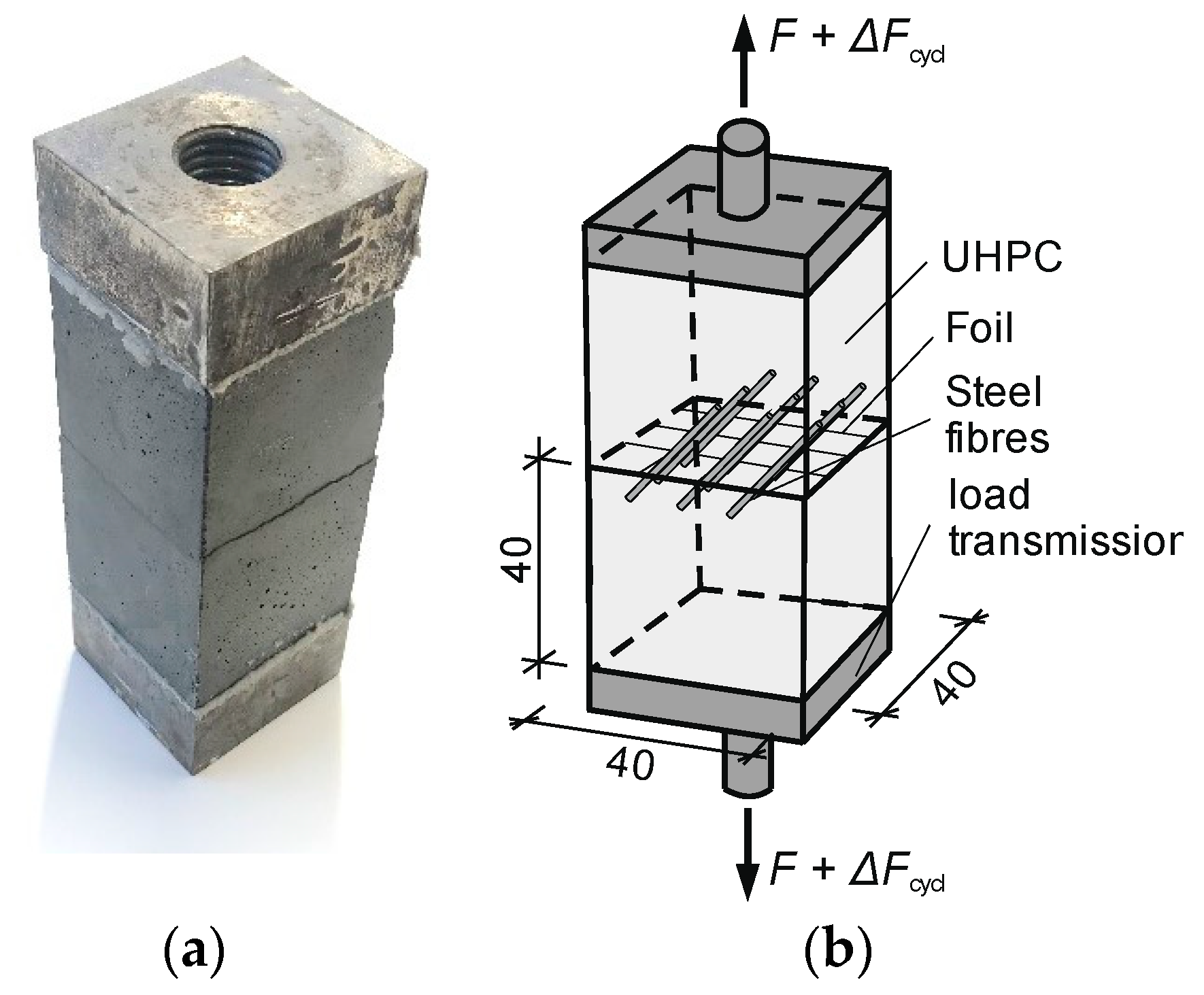
4. Experimental Program
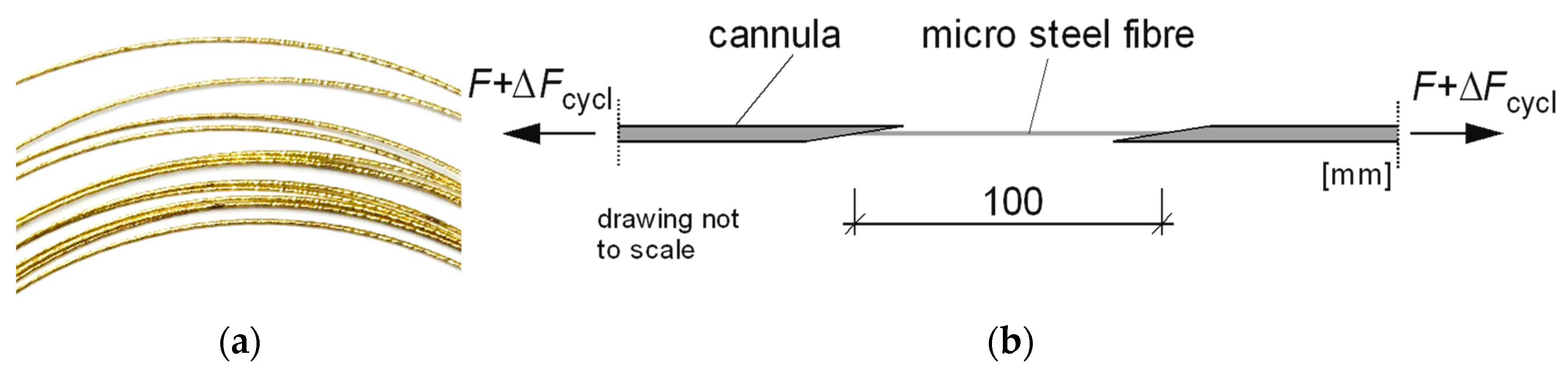
4.1. Test Specimen and Test Configuration
4.2. Monotonic Loading
4.3. Cyclic Loading
5. Fibre Groups Embedded in UHPC
5.1. Test Specimen and Test Programme
5.2. Monotonic Tensile Loading
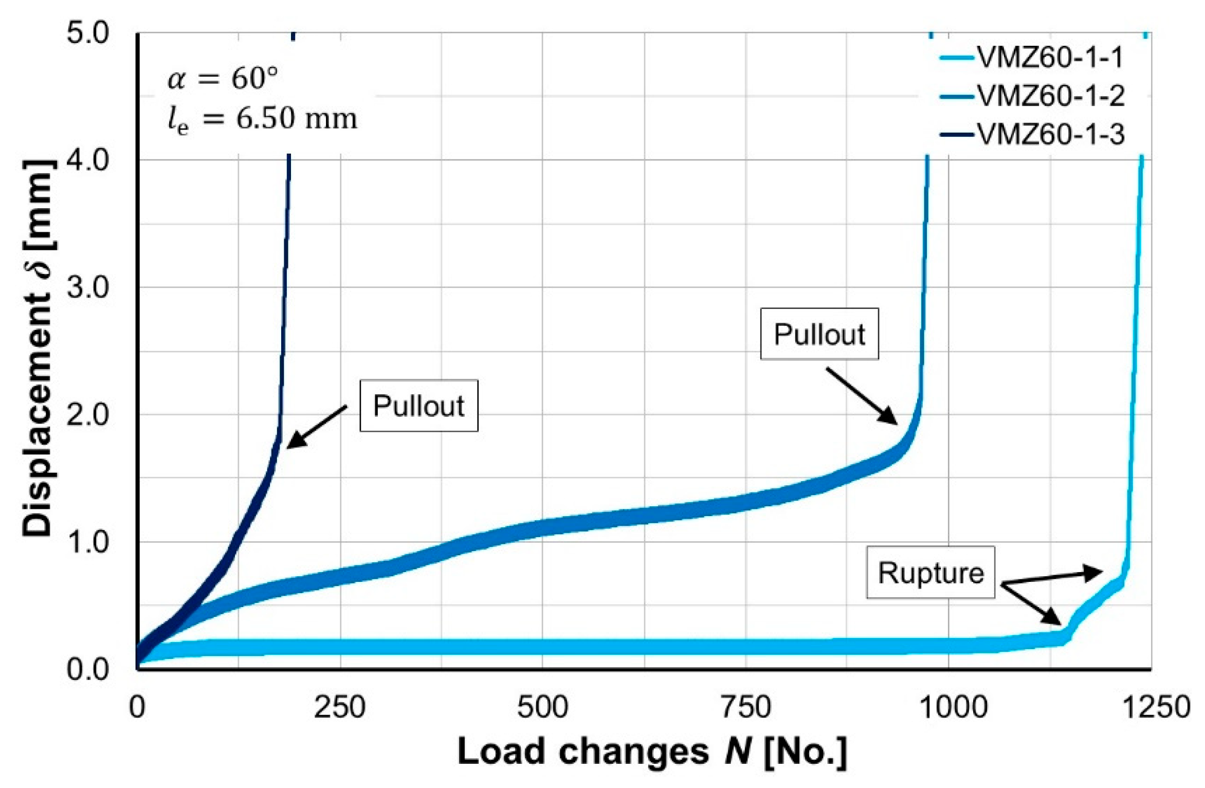
5.3. Cyclic Tensile Loading
- Phase I marks the initial non-linear increase in strain.
- Phase II begins between 5% and 10% of the ultimate load cycle number with the transition to a constant, small increase in deformation.
- Phase III is reached at around 95% of the breaking load cycle number . The total deformations increase rapidly, disproportionately, leading to failure of the concrete.
- This type of failure would actually have been expected with a fibre orientation of 30°, because greater bending stresses occur in the steel fibre compared to an orientation of 60° (cf. Figure 9). The following explanation can be given for this:
- With a fibre orientation of 30°, no fibre breakage occurs because the “snubbing effect” causes a larger concrete breakout, which in turn considerably shortens the bond length. This reduces the bending stresses on the one hand and increases the bond stresses on the other. The latter causes the fatigue damage of the bond zone to progress faster than the material damage. This eventually leads to fibre pullout.
- With 60°-inclined fibres, on the other hand, the “snubbing effect” leads to less concrete breakout and the bond length is reduced less (in comparison to a fibre orientation of 30°). The relationship between the damage of the bond zone and the fibre material (bending effects) is in an indifferent state, where both fibre pullout (VMZ60-1) and fibre breakage (VMZ60-2) can occur. Both failure modes can also be seen in Figure 12.
6. Conclusions and Outlook
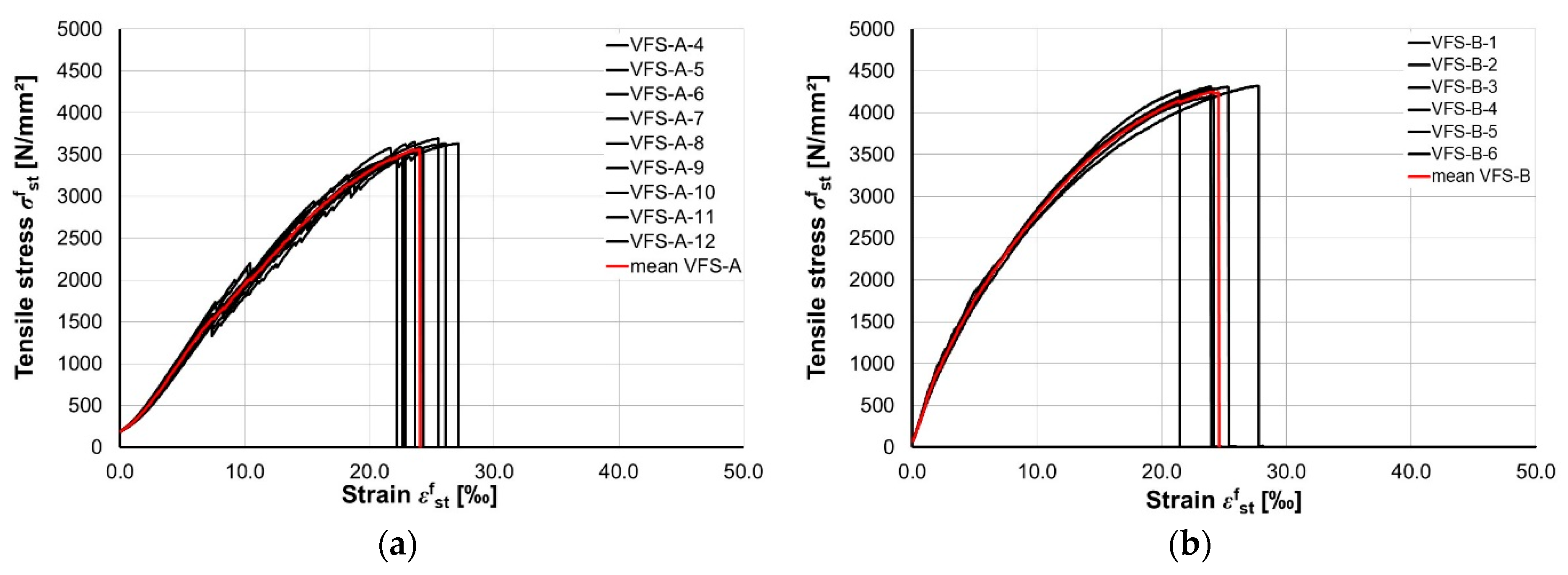
- The stress–strain relationship of the high-strength micro steel fibres showed no considerable ductility like conventional steel. The failure is brittle.
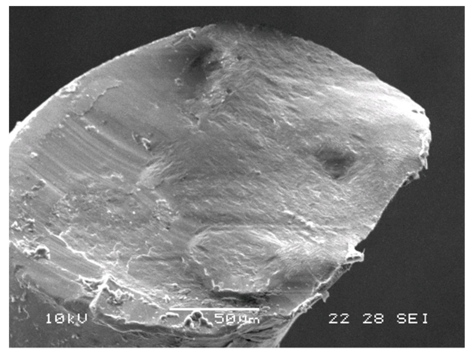
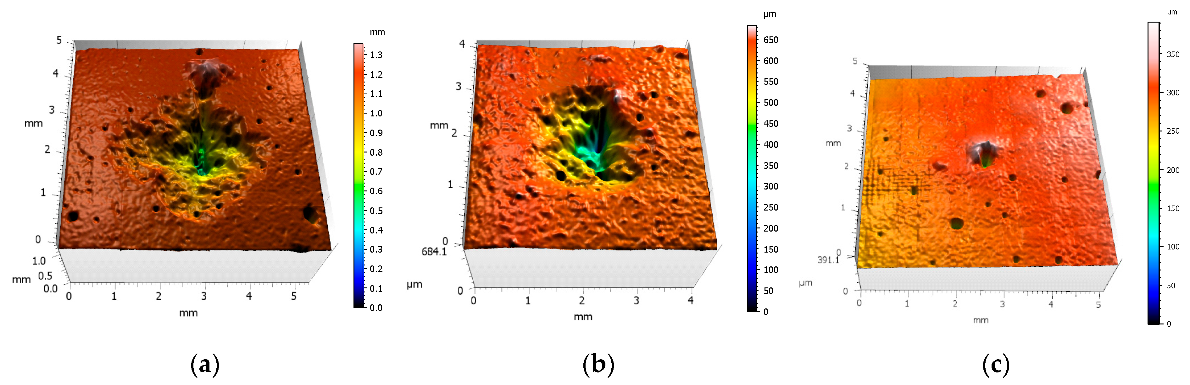
- The brass coating of the high-strength micro steel fibre hides gouges located in the longitudinal direction of the fibre underneath. The gouges reduce the cross-sectional insignificantly and do not affect the tensile strength in a considerable manner.
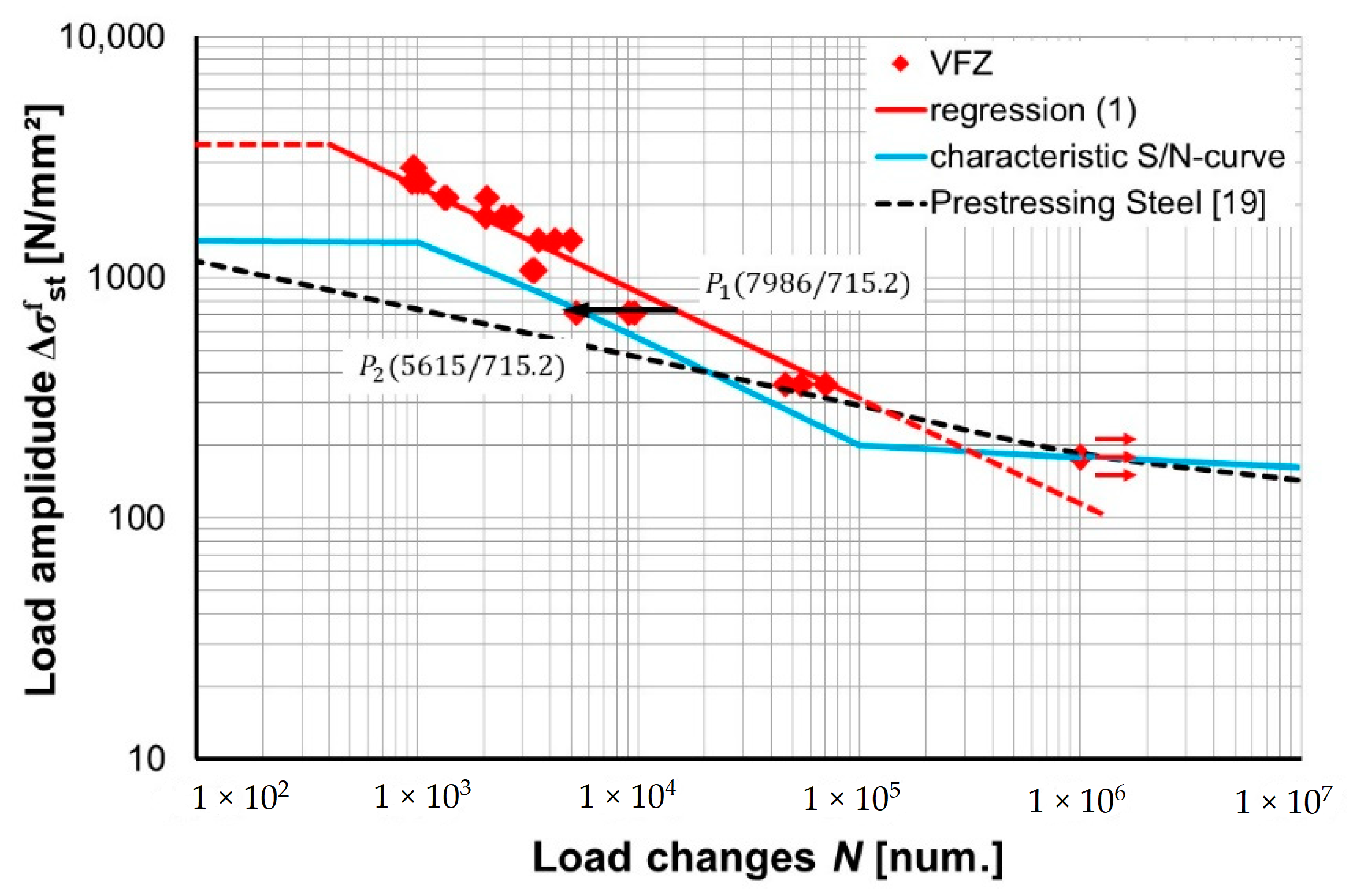
- The mean S/N curve of the high-strength micro steel fibre showed in the first instance no good agreement with prestressing steel. After converting the mean S/N curve into characteristic values, a comparison with prestressing steel was possible and provided relatively good agreement for the high-cycle fatigue. Equation (4) provides a recommendation for a mathematical formulation of the S/N curve.
- The used high-strength steel fibres always pulled out of the concrete matrix under monotonic loading, i.e., no fibre rupture occurred. The maximal pullout resistance in the test program was approximately one-third of the fibre’s tensile strength. After the peak load, the pullout curves show an almost linear decreasing course of curves.
- Under cyclic loading, fibre rupture occurred partly at orientations of 60° but not for 30° and 90°. The fatigue curves of the un-cracked micro steel fibres showed the typical course of curves like fatigue of concrete: strain stabilisation, linear strain increase, and exponential strain increase.
Author Contributions
Funding
Acknowledgments
Conflicts of Interest
References
- Schmidt, M. Sustainable Building with Ultra-High-Performance Concrete (UHPC)—Coordinated Research Program in Germany. In Proceedings of the Hipermat 2012, 3rd International Symposium on UHPC and Nanotechnology for High Performance Construction Materials, Kassel, Germany, 7–9 March 2012; pp. 17–25. [Google Scholar]
- Graybeal, B.A. Ultra-High Performance Concrete: A State-of-the-Art Report or the Bridge Community; United States Federal Highway Administration: McLean, VA, USA, 2013.
- Schweizerischer Ingenieur- und Architektenverein (SIA). Ultra-Hochleistungs-Faserbeton (UHFB)—Baustoffe, Bemessung und Ausführung; SIA: Zurich, Switzerland, 2016; Volume 1. [Google Scholar]
- Association Francaise de Normalisation (AFNOR). National Addition to Eurocode 2—Design of Concrete Structures: Specific Rules for Ultra-High Performance Fibre-Reinforced Concrete (UHPFRC); Association Francaise de Normalisation (AFNOR): Paris, France, 2016. [Google Scholar]
- Fahrat, F.A. High-performance fibre-reinforced cementitious composites (CARDIFRC)—Performance and application to retrofitting. Eng. Fract. Mech. 2007, 74, 151–167. [Google Scholar]
- Graybeal, B.A.; Hartman, J.L. Ultra-High Performance Concrete Material Properties. In Proceedings of the 2003 Transportation Research Board Conference, Washington, DC, USA, 12–16 January 2003. [Google Scholar]
- Behloul, M.; Chanvillard, G.; Pimienta, P.; Pineaud, A.; Rivillon, P. Fatigue Flexural Behavior of Pre-Cracked Specimens of Special UHPFRC; American Concrete Institute: Lansing, MI, USA, 2005; Volume 228, pp. 1253–1268. [Google Scholar]
- Abrishambaf, A.; Pimentel, M.; Nunes, S. A meso-mechanical model to simulate the tensile behaviour of ultra-high performance fibre-reinforced cementitious composites. Compos. Struct. 2019, 222, 110911. [Google Scholar] [CrossRef]
- Cao, Y.; Yu, Q.; Brouwers, H.; Chen, W. Predicting the rate effects on hooked-end fiber pullout performance from Ultra-High Performance Concrete. Cem. Concr. Res. 2019, 120, 164–175. [Google Scholar] [CrossRef]
- McSwain, A.C.; Berube, K.A.; Cusatis, G.; Landis, E.N. Confinement effects of fiber pullout forces for ultra-high-performance concrete. Cem. Concr. Compos. 2018, 91, 53–58. [Google Scholar] [CrossRef]
- Wille, K.; Naaman, A.E. Effect of Ultra-High-Performance Concrete on Pullout Behaviour of High-Strength Brass-Coated Steel Fibers. ACI Mater. J. 2013, 110, 451. [Google Scholar]
- Matika, T.; Brühwiler, E. Tensile fatigue behaviour of ultra-high performance fibre reinforced concrete (UHPFRC). Mater. Struct. 2014, 47, 475–491. [Google Scholar] [CrossRef]
- Lappa, E.S. High Strength Fibre Reinforced Concrete: Static and Fatigue Behaviour in Bending. Ph.D. Thesis, TU Delft, Delft, The Netherlands, 28 June 2007. [Google Scholar]
- Bornemann, R.; Faber, S. UHPC with steel- and non-corroding high-strength polymer fibres under static and cyclic loading. In Proceedings of the International UHPC Symposium, Kassel, Germany, 13–15 September 2004; pp. 673–682. [Google Scholar]
- Oettel, V.; Lanwer, J.-P.; Empelmann, M. Auszugverhalten von Mikrostahlfasern aus UHPC unter monoton steigender und zyklischer Belastung. Bauingenieur 2021, 96, 1–10. [Google Scholar] [CrossRef]
- Stürwald, S. Versuche zum Biegetragverhalten von UHPC mit Kombinierter Bewehrung; Forschungsbericht; Fachgebiet Massivbau, Fachbereich Bauingenieurwesen, Universität Kassel: Kassel, Germany, 2011. [Google Scholar]
- Lanwer, J.-P.; Oettel, V.; Empelmann, M.; Höper, S.; Kowalsky, U.; Dinkler, D. Bond behaviour of micro streel fibres embedded in ultra-high performance subjected to monotonic and cyclic loading. Struct. Concr. 2019, 20, 1243–1253. [Google Scholar] [CrossRef]
- Radaj, D.; Vormwald, M. Ermüdungsfestigkeit. 3. Auflage; Springer: Berlin/Heidelberg, Germany, 2007. [Google Scholar]
- Fib—Fédération Internationale du Béton. Fib Model Conde for Concrete Structures; Ernst & Sohn: Berlin, Germany, 2013. [Google Scholar]
- Yoo, D.-Y.; Park, J.-J.; Kim, S.-W. Fiber pullout behavior of HPFRCC: Effects of matrix strength and fiber type. Compos. Struct. 2017, 174, 263–276. [Google Scholar] [CrossRef]
- Abdallah, S.; Fan, M.; Cashell, K.A. Pull-out behaviour of straight and hooked-end steel fibres under elevated temperatures. Cem. Concr. Res. 2017, 96, 132–140. [Google Scholar] [CrossRef]
- Li, V.C.; Baker, S. Effect of inclining angle, bundling and surface treatment on synthetic fibre pull-out from a cement matrix. Composites 1990, 21, 132–140. [Google Scholar] [CrossRef]
- Empelmann, M.; Oettel, V.; Lanwer, J.-P.; Dinkler, D.; Kowalsky, U.; Höper, S. Cyclic Deterioration of Bond Zone between Fibres and UHPC. In Proceedings of the HiPerMat, Kassel, Germany, 11–13 March 2020; pp. 141–142. [Google Scholar]


| Name | Number | Diameter | Ultimate Tensile Strength | Ultimate Strain |
|---|---|---|---|---|
| [-] | [Num.] | [mm] | [N/mm2] | [‰] |
| VFS-A | 9 | 0.19 | 3575.8±80.2 | 22.8±0.7 |
| VFS-B | 6 | 0.13 | 4250.4±95.2 | 24.6±2.3 |
| Name | Tensile Strength | Standard Deviation | 5%-Quantile of | |
|---|---|---|---|---|
| [-] | [mm] | [N/mm2] | [N/mm2] | [N/mm2] |
| VFS-A | 0.19 | 3575.8 | 80.2 | 3462.4 |
| VFS-B | 0.13 | 4250.4 | 95.2 | 4080.7 |
| Name | Quantity | Upper Stress Level | Lower Stress Level | Load Amplitude | Load Amplitude | Load Cycles |
|---|---|---|---|---|---|---|
| [-] | [num.] | [-] | [-] | [-] | [N/mm2] | [num.] |
| VFZ-1 | 3 | 0.90 | 0.10 | 0.80 | 2860.7 | 962±5 |
| VFZ-2 | 3 | 0.80 | 0.10 | 0.70 | 2503.1 | 1008±46 |
| VFZ-3 | 3 | 0.70 | 0.10 | 0.60 | 2145.5 | 1593±344 |
| VFZ-4 | 3 | 0.60 | 0.10 | 0.50 | 1787.9 | 2382±260 |
| VFZ-5 | 3 | 0.50 | 0.10 | 0.40 | 1430.3 | 4240±580 |
| VFZ-6 | 3 | 0.40 | 0.10 | 0.30 | 1072.7 | 3364±40 |
| VFZ-7 | 3 | 0.30 | 0.10 | 0.20 | 715.2 | 7986±1963 |
| VFZ-8 | 3 | 0.20 | 0.10 | 0.10 | 357.6 | 57,375±10,073 |
| VFZ-9 | 3 | 0.15 | 0.10 | 0.05 | 178.8 | 1,000,000±0 |
| Reinforcing Steel Bars: | High-Strength Micro Steel Fibre: | |
|---|---|---|
| ||
| ||
|
| Components | UHPC-1017 |
|---|---|
| [-] | [kg/m3] |
| Cement CEM I | 795.0 |
| Silica fume | 168.6 |
| Superplasticiser | 24.1 |
| Quartz powder | 198.4 |
| Quartz sand 0.125/0.5 mm | 971.0 |
| Water | 189.9 |
| Name | Number | Orientation | Length | Max. Pullout Resistance | Displacement at Max. | Load Changes Num | Failure Mode |
|---|---|---|---|---|---|---|---|
| [-] | [No.] | [°] | [mm] | [N/mm2] | [mm] | [No.] | [-] |
| VMS30-1 | 3 | 30° | 3.25 | 376.9±41.2 | 1.46 | - | Pullout |
| VMS30-2 | 3 | 6.50 | 993.6±66.6 | 2.28 | - | Pullout | |
| VMS60-1 | 3 | 60° | 3.25 | 480.7±71.0 | 0,63 | - | Pullout |
| VMS60-2 | 3 | 6.50 | 1176.3±26.7 | 0.60 | - | Pullout | |
| VMS90-1 | 3 | 90° | 3.25 | 568.7±42.4 | 0.45 | - | Pullout |
| VMS90-2 | 3 | 6.50 | 1159.1±53.3 | 0.50 | - | Pullout | |
| VMZ30-1 | 3 | 30° | 3.25 | - | - | 158±116 | Pullout |
| VMZ30-2 | 3 | 6.50 | - | - | 250±42 | Pullout | |
| VMZ60-1 | 3 | 60° | 3.25 | - | - | 88±19 | Pullout |
| VMZ60-2 | 3 | 6.50 | - | - | 848±442 | Pullout/Rupture | |
| VMZ90-1 | 3 | 90° | 3.25 | - | - | 455±399 | Pullout |
| VMZ90-2 | 3 | 6.50 | - | - | 373±12 | Pullout | |
| ∑ 36 | |||||||
Publisher’s Note: MDPI stays neutral with regard to jurisdictional claims in published maps and institutional affiliations. |
© 2021 by the authors. Licensee MDPI, Basel, Switzerland. This article is an open access article distributed under the terms and conditions of the Creative Commons Attribution (CC BY) license (https://creativecommons.org/licenses/by/4.0/).
Share and Cite
Lanwer, J.-P.; Empelmann, M. Fundamental Investigations on the Performance of Micro Steel Fibres in Ultra-High-Performance Concrete under Monotonic and Cyclic Tensile Loading. Appl. Sci. 2021, 11, 9377. https://doi.org/10.3390/app11209377
Lanwer J-P, Empelmann M. Fundamental Investigations on the Performance of Micro Steel Fibres in Ultra-High-Performance Concrete under Monotonic and Cyclic Tensile Loading. Applied Sciences. 2021; 11(20):9377. https://doi.org/10.3390/app11209377
Chicago/Turabian StyleLanwer, Jan-Paul, and Martin Empelmann. 2021. "Fundamental Investigations on the Performance of Micro Steel Fibres in Ultra-High-Performance Concrete under Monotonic and Cyclic Tensile Loading" Applied Sciences 11, no. 20: 9377. https://doi.org/10.3390/app11209377
APA StyleLanwer, J.-P., & Empelmann, M. (2021). Fundamental Investigations on the Performance of Micro Steel Fibres in Ultra-High-Performance Concrete under Monotonic and Cyclic Tensile Loading. Applied Sciences, 11(20), 9377. https://doi.org/10.3390/app11209377