SLA-DQTS: SLA Constrained Adaptive Online Task Scheduling Based on DDQN in Cloud Computing

Abstract

Task scheduling is key to performance optimization and resource management in cloud computing systems. Because of its complexity, it has been defined as an NP problem. We introduce an online scheme to solve the problem of task scheduling under a dynamic load in the cloud environment. After analyzing the process, we propose a server level agreement constraint adaptive online task scheduling algorithm based on double deep Q-learning (SLA-DQTS) to reduce the makespan, cost, and average overdue time under the constraints of virtual machine (VM) resources and deadlines. In the algorithm, we prevent the change of the model input dimension with the number of VMs by taking the Gaussian distribution of related parameters as a part of the state space. Through the design of the reward function, the model can be optimized for different goals and task loads. We evaluate the performance of the algorithm by comparing it with three heuristic algorithms (Min-Min, random, and round robin) under different loads. The results show that the algorithm in this paper can achieve similar or better results than the comparison algorithms at a lower cost.

1. Introduction

With the rapid development of computer technology and the internet economy, cloud computing, as the cornerstone of big data and artificial intelligence (AI), is one of the most promising and valuable research directions, and efficient task scheduling has always been the goal and challenge of research in this field [1]. Considering that the services and resources provided by cloud service providers have increased significantly in the past ten years, and their workloads exhibit a high degree of dynamic change, how to adapt to the online task scheduling environment with dynamic changes has become an important issue [2].

AI is an emerging research topic, and it can be used to solve complex problems and find optimized solutions in many applications and fields. Hence, it can potentially solve the task scheduling problem in software as a service (SaaS). The benefits of AI in science, medicine, technology, and the social sciences have been proven. With the popularity and development of cloud computing, the process of task scheduling will generate a large number of records, and these data can be used to establish a data-driven AI task scheduling system. Training through the data continuously generated during scheduling helps in the formation of strategies according to the current environment. Although AI technology has made significant progress, its use in systems that require reliability, transparency, and maintainability is still in its infancy.

Task scheduling and resource allocation in the cloud environment usually have the optimization goals of reducing makespan, improving resource utilization, load balancing, cost optimization, and reducing energy consumption [3]. Previous studies have proposed a solution for scheduling optimization for one goal or even multiple goals [4]. Practical research must consider multiple cloud computing task scheduling objectives. Current methods can be categorized as heuristic algorithms, meta-heuristic algorithms, and reinforcement learning (RL) [5]. Most schemes consider the scheduling of offline batch tasks, and cannot be applied to dynamically changing workloads in online task scheduling [2].

We model the online task scheduling problem of cloud computing and propose server-level agreement constraint adaptive online task scheduling algorithm based on double deep Q-learning (SLA-DQTS), an algorithm based on deep reinforcement learning (DRL) [6] under server level agreement (SLA) constraints. We consider the dynamic change of the cloud computing environment and task load through the design of the state space and reward function to adaptively learn the scheduling strategy between the task load and number of VMs, and we use reinforcement learning to maximize the cumulative reward to acquire a long-term decision-making strategy. The main contributions of this work are summarized as follows:

•

With the widespread application of DRL in task scheduling, we propose an intelligent task scheduling framework using DDQN in cloud computing online task scheduling to optimize the allocation decision of online tasks to virtual machines (VM). In the makespan and cost optimization problems under the constraints of the SLA, the corresponding scheduling strategy is learned according to the load situation.

•

Considering the dynamics of the cloud environment, we design a state-action space and reward function. As the environment load changes, the reward function switches the main optimization goal. Using the Gaussian distribution of related features as the state space, the input dimension of the model remains unchanged under different numbers of VMs. The reward function allows the model to adapt to changes in the task load. The fixed-dimensional state space makes it unnecessary to change the model with the number of VMs.

The rest of this article is organized as follows. Related research is discussed in Section 2. Section 3 introduces the key stages of online task scheduling and proposes a problem model. Section 4 introduces the design of the algorithm, and Section 5 discusses our simulation experiments to test its performance. Section 6 relates our conclusions and discusses our future work.

2. Related Work

Since there is no effective polynomial algorithm, task scheduling is a well-known NP problem [7]. For this reason, researchers have proposed many algorithms for related problems to obtain suitable solutions, whose optimization goal is usually to minimize the makespan and cost. With the development of AI technology, reinforcement learning (RL) is being used to solve this problem. RL possesses general intelligence sufficient to solve some complex problems, and has reached the human level in some chess, card, and electronic games.

Heuristic methods prioritize generality and are easy to understand and implement, but they are not self-adaptive and cannot adjust strategies according to the corresponding environment to achieve ideal performance [8]. Min-Min and Max-Min are well-known heuristic scheduling algorithms that assign smaller and larger tasks, respectively, to VMs with fast processing speed [9]. Pan et al. [10] proposed a critical-path-duration-estimation-based (CPDE) VM selection strategy to address the performance-variation-aware workflow scheduling problem. Mboula et al. [11] proposed cost–time trade-off efficient workflow scheduling (CTTWS) to minimize both user-defined budgets and deadlines in commercial cloud environments. Zhao et al. [12] proposed dynamic workflow scheduling based on autonomic fault-tolerant scheme selection in uncertain environments. Lin et al. [13] proposed a hierarchical iterative application partition (HIAP) to partition an application into a set of dependent tasks, cooperating with online scheduling algorithms to finish workflows with a low average payment.

Particle swarm optimization (PSO), ant colony optimization (ACO), and genetic algorithms (GAs) are commonly used in metaheuristics. Rodriguez et al. [14] proposed a PSO algorithm based on metaheuristic optimization to minimize the overall execution cost of a workflow while meeting deadline constraints. Chen et al. [15] proposed soft real-time task scheduling based on PSO for cloud computing to maximize profits while meeting deadlines considering load balancing. Chen et al. [16] proposed PSO based on an AC algorithm, which performed well in terms of cost, makespan, convergence, and results. Hall et al. [17] proposed a dynamic task scheduling algorithm (IGATS) based on an improved GA, considering the dynamic characteristics of the cloud computing environment, and introduced the concept of load priority. Good performance was achieved in terms of response and execution times. Al-Zoubi et al. [18] proposed a grasshopper optimization algorithm (GOA) to reduce makespan. Reddy et al. [19] proposed a regressive whale optimization (RWO) algorithm for workflow scheduling in a cloud computing environment to reduce the time and cost of execution. Khodar et al. [20] proposed a PSO-based multipurpose algorithm to optimize task-transfer and execution times at the least expense. Zhou et al. [21] proposed a task scheduling optimization algorithm, modified PSO (M-PSO), to handle the local optimum and slow convergence problem. Chen et al. [22] proposed an exact formulation based on linear programming to produce optimal allocation schemes for tasks, and a population-based approach to allocate tasks to resources to minimize the total time cost.

RL is a process in which agents make action decisions through learning to maximize cumulative reward. Barrett et al. [23] showed the initial architecture of a cloud workflow scheduler and the preliminary results of combining RL technology to efficiently schedule workflows in the cloud computing environment in the form of continuous state-action space to minimize monetary costs under deadlines. Aiming at the precisely scaled cloud computing environment and efficient task scheduling under resource constraints, Peng et al. [24] proposed a task scheduling scheme. They used RL to develop a cloud computing scheduling model and optimize the response time under given cloud computing resources to minimize problem. The experimental results show that the proposed task scheduling scheme can optimize cloud resource utilization and load balancing to obtain the minimum response time under resource constraints. Xiao et al. [25] aimed at hybrid cloud, which is a joint service of multiple clouds. They modeled the problem of each scheduler as MDP, proposed a hybrid cloud distributed scheduling algorithm, and used Q-learning to obtain a suitable scheduling strategy. The result proves that compared with the five typical dynamic scheduling algorithms (opportunistic load balancing, shortest execution time, shortest completion time, handover algorithm, and k-percent best), the scheme has a short average response time and high collaboration efficiency. Soualhia et al. [26] proposed a dynamic, fault-aware framework that can be integrated into a Hadoop scheduler. The framework relies on ML algorithms and a Markov decision process (MDP) to generate scheduling strategies. The framework was deployed with ATLAS+, an adaptive fault-aware scheduler for Hadoop. The performance of ATLAS+ was compared with that of the FIFO, Fair, and Capacity Hadoop schedulers, and it was found to be better in terms of the number of failed jobs, total execution time, and resource utilization. Riera et al. [27] describes TeNOR, a micro-service-based network function virtualization orchestrator capable of effectively addressing resource and network service mapping. One of the resource mapping strategies uses reinforcement learning. Through iterative learning of the best strategy for resource mapping, the acceptance rate of the RL method in large-scale NS has increased significantly in experiments.

People have gradually turned their attention to DRL, with its potential for long-term learning and decision making, and it has been applied to some scheduling problems in cloud computing. Jayswal [28] proposed GA-ANN, a neural-network-based scheduling algorithm providing better QoS. Kaur et al. [29] proposed the DQ-HEFT algorithm, combining DRL and the heterogeneous earliest completion time algorithm, using DQL for task sequencing and heterogeneous earliest finish time (HEFT) for task allocation. Cui et al. [30] proposed a job scheduling scheme based on RL to optimize VM resources and deadlines while minimizing the construction time and average waiting time (AWT). Tong et al. [31] proposed an AI algorithm, deep Q learning task scheduling (DQTS), to solve the task scheduling problem of a directed acyclic graph (DAG). Li et al. [32] proposed a deep job scheduling (DeepJS) algorithm based on deep reinforcement learning to minimize makespan, and proved its convergence and generalization. Ran et al. [2] proposed a deep deterministic gradient strategy (DDPG) to find the optimal allocation plan that meets the requirements of the SLA and minimizes the average response time. It performed well at reducing average response time and balancing loads. Dong et al. [33] proposed a task scheduling algorithm based on a deep reinforcement learning architecture (RLTS) to minimize the task execution time.

RL technology has been widely used in cloud computing, but the huge state space and action space of the cloud computing system make the traditional RL technology inapplicable [34]. Therefore, DRL technology has also begun to emerge in this area, and has shown its ability to solve high-dimensional problems.

3. Proposed Online Task Scheduling Model

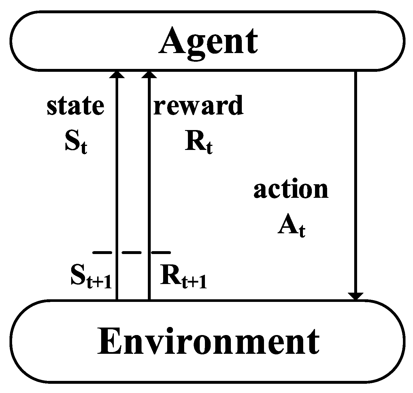
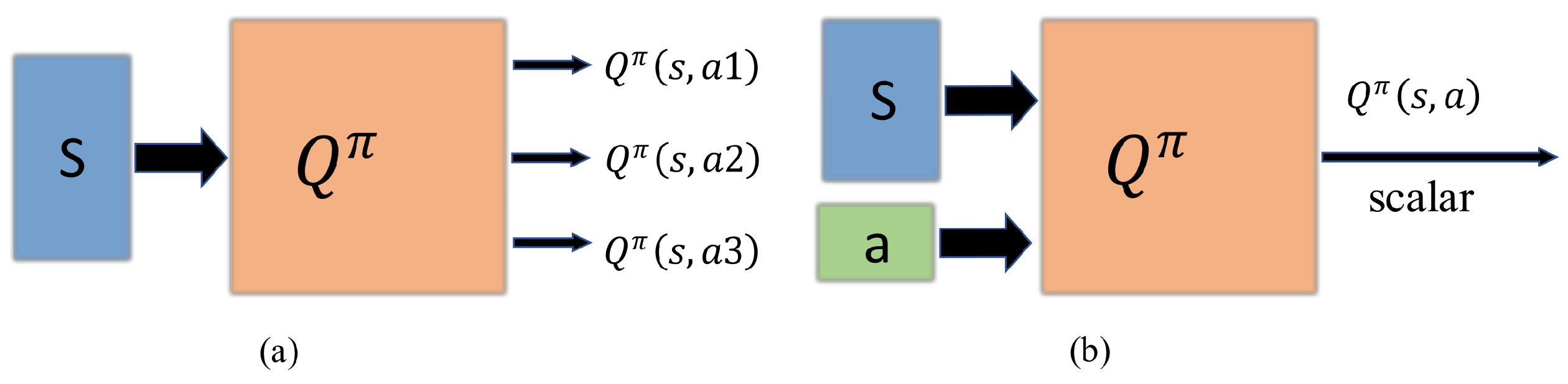
3.1. Deep Learning Technique

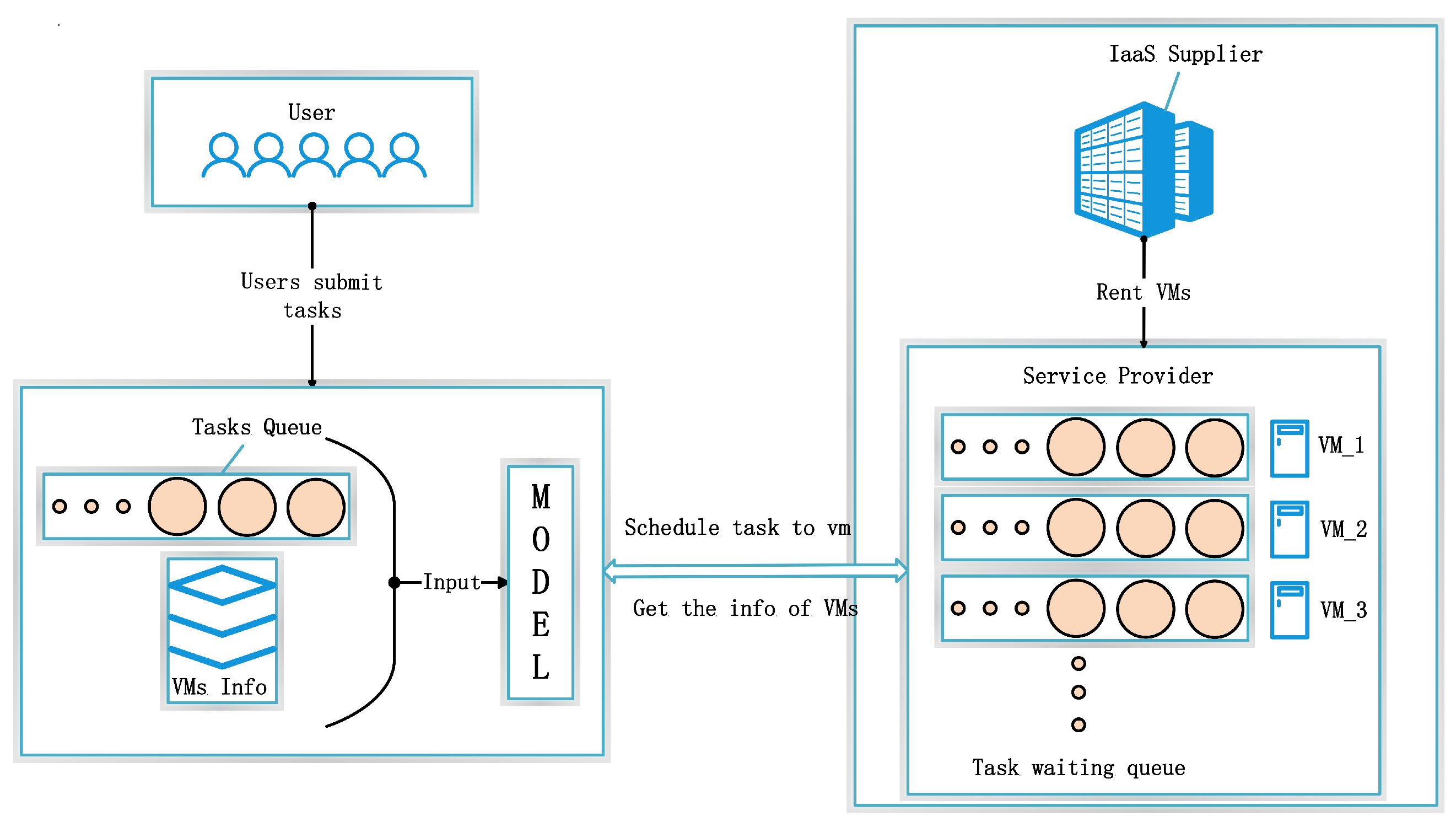
RL is a branch of ML, which learns continuously through the agent’s interaction with the environment based on the rewards or punishments obtained, to better adapt to the environment [35]. RL can learn without a priori knowledge of the environment and obtain the decision-making ability of the corresponding environment through repeated interactive learning. Figure 1 shows a classic RL model. In each step, the agent makes a decision based on the strategy $\pi$ through the state $S_t$ obtained from the environment and takes action $a=\pi \left(s\right)$. The environment transfers accordingly from state $S_t$ to state $S_{t+1}$. The agent obtains $R_t$ returned by this process. RL assumes the process has a Markov property, i.e., the probability and reward of state transition only depend on $S_t$ and $A_t$, and have nothing to do with the state action before $t-1$. Through interaction with the environment, the agent can record these quantities for learning, so as to maximize the expected cumulative reward $G_t$. Therefore, RL can obtain decision-making strategies through observation and learning without prior knowledge of the environment.

The strategy used by the agent to make decisions in RL is defined by the probability distribution $\pi \left(a\right|s)$ of action a under state s. In the classic reinforcement learning algorithm Q-learning, it is composed of state and action. Q-table is used for storage, and the s-a mapping with the highest Q-value in state s is selected from the table when making a decision.

In Q-learning, the optimal strategy is that ${arg\; max}_{a\in A}\left(Q\left(a\right|S_t)\right)$ is the maximum cumulative return of the selection action an in state $S_t$. If Q can predict the cumulative return of each action in the current state, the optimal decision can be made. The following is the updated formula of Q:

$$Q(S_t,A_t)=Q(S_t,A_t)+\alpha [R_t+\lambda ma{x}_{a}Q(S_{t+1},a)-Q(S_t,A_t)]$$

(1)

The $R_t$ is the return of the action $A_t$ in the state $S_t$. The $\lambda$ is the discount factor, which is used to calculate the cumulative return. Take the currently observed return $R_t$ plus $\lambda$ multiplied by the maximum cumulative return of the next state $S_{t+1}$ as the current maximum cumulative return. Make the difference between it and the expected return of the current state $S_t$ to obtain the loss, and multiply the loss by the learning factor $\alpha$ to update the current prediction value. After repeated iterations, the more accurate the prediction of Q, the smaller the loss value, and the more stable the value predicted by Q until convergence. At the same time, to make the algorithm converge faster and more stable, it needs suitable training samples, a suitable exploration strategy. The most common strategy is the $ϵ$-greedy policy, which is a simple strategy. During exploration, it is determined whether to randomly select an action or choose the action with the highest return under Q prediction according to the probability $ϵ$. In the early stage of training, a higher $ϵ$ value is required to enhance the exploration to accelerate the convergence. In the later stage, the $ϵ$ value can be reduced to increase the convergence accuracy.

Actual problems have a large number of state actions. It is inappropriate to store the probability distribution in the form of a table, and if a state has never appeared, Q-learning cannot handle it. That is, it lacks generalization ability, so a function with a certain number of parameters is generally used for fitting. As the amount of data and number of features increase, the advantages of deep neural networks have become more obvious, and DRL, which combines deep neural networks and RL, has achieved good results in many fields. The algorithm prototype based on this article, the deep Q network (DQN) [6], combines deep neural networks and Q-learning. Q-table is fitted through a deep neural network to solve the problem of excessive state space.

3.2. System Model

Our task scheduling system considers a common cloud computing scenario, SaaS. It includes users who submit tasks, service providers, and IaaS providers [36]. Service providers build their resource pools from VM instances rented by IaaS providers, and provide users with services through the network. Service providers receive various types of tasks submitted by end-users through the network. An efficient and flexible task scheduler that can take into account multiple goals is necessary to balance the profit of the service provider against the user experience (e.g., response time and throughput).

In cloud computing, tasks submitted by users are allocated to cloud nodes based on a set scheduling strategy. Hence, the choice of scheduling strategy is important to the task completion time and cost. Figure 2 shows the online dynamic task scheduling model of a typical cloud computing scenario. The user can submit a task at any time. After submission, the scheduling center allocates a task to the task waiting queue of the VM according to its demand and the scheduling strategy. We proposed SLA-DQTS for this process. It uses the virtual machine and task information obtained by the scheduler to determine the VM that executes the task. After the decision, the task is added to the task waiting queue of the selected VM. We stipulate that each VM maintains its task waiting queue, and processes tasks in a first-come-first-served manner and space share model according to the queue. The VM processes the tasks in a first-come-first-served manner according to the task queue. In this article, tasks whose number and resource requirements are unknown are dynamically submitted to the scheduler. We take scheduling time, cost, and SLA as optimization goals, and design a scheduling plan that can adapt to different loads.

In our problem model, users can submit any number of tasks at the same time, which do not require consistent resource requirements, and can be of multiple types. Therefore, the submission time, number, and type are unpredictable. Application service providers can change the numbers of VMs according to the load, so we consider the adaptation of the model to a variable number of VMs.

The scheduling center can obtain the status information of all VMs, including tasks in the queue. After a task arrives, the scheduling center reads its resource demand, calculation amount, and expected completion time, and matches it to a VM. At the end of each batch of tasks, the scheduling center records decisions and task execution-related results, such as VMs assigned to tasks, starting and ending execution times, and costs.

3.3. Problem Formulation

Our simulation environment is somewhat simplified. We consider the task-related attributes of million instructions per second (MIPS), bandwidth, amount of calculation, bandwidth transmission, and expected completion time, and ignore failure situations that may occur in the real environment. Tasks arrive at the data center in batches, and their arrival times conform to a Poisson distribution. The number of tasks and resource requirements in different batches of tasks are randomly generated within a certain range. The scheduler assigns a task to the task cache queue of the appropriate machine.

Tasks are submitted online. The scheduler cannot predict resource requirements and numbers of tasks. Based on this assumption, we define that a batch can contain multiple tasks, expressed as $CLU\_T=\left\{t_i|i\in N+\right\}$, where $\left|CLU\_T\right|$ is the number of tasks in a batch. Each task can be expressed as

$$t_i=\left\{\begin{array}{c}{t}_i^{mips},t_i^{bw},t_i^{mips\_l}{t}_i^{bw\_l},t_i^{dead}\\ t_i^{load},t_i^{finish}{t}_i^{start},t_i^{cost}\end{array}\right\},$$

(2)

where i is the number of a task; $t_i^{mips}$ and $t_i^{bw}$ respectively represent the task’s requirements for computing and bandwidth resources; $t_i^{mips\_l}$, $t_i^{bw\_l}$ respectively indicate the lengths of tasks corresponding to computing and bandwidth resources; $t_i^{dead}=\frac{t_i^{mips\_l}}{t_i^{mips}}+\frac{t_i^{bw\_l}}{t_i^{bw}}$ indicates the task processing time expected by the user; $t_i^{load},t_i^{start},t_i^{finish}$, and $t_i^{cost}$ are respectively the time when a task is submitted, time the task is executed by the node, time the task is completed, and execution cost. Prices differ according to the resources of VMs, so the cost of a task is determined by the VM and the execution time.

After submission to the data center, a task is scheduled to the VM, which will be occupied until the end of execution, with no preemption. The VM set in the cluster is defined as $CLU\_VM=\left\{{vm}_j|j\in N+\right\}$, where $\left|CLU\_VM\right|$ is the number of the VM. A VM instance is defined as

$${vm}_j=\left\{{vm}_j^{mips},{vm}_j^{bw},{vm}_j^{price}\right\},$$

(3)

where j is the number of the VM, ${vm}_j^{mips}$ is the number of instructions per second executed by the VM, ${vm}_j^{bw}$ is the bandwidth of the VM, and ${vm}_j$ can perform the task only when

$$\begin{array}{c}\hfill {t_i^k\le vm}_j^k\forall k\in \left[mips,bw\right]\end{array},$$

(4)

where ${vm}_j^{price}$ is the price per hour of a VM. We refer to Alibaba cloud resource pricing to determine pricing. Computing resources have linear pricing, bandwidth resources have tiered pricing, and the price ratio (this article is set as 0.0003/MIPS, (0.063,0.248)/mb) is calculated as

$$\begin{array}{cc}\hfill {vm}_{mips}^{price}& ={vm}^{mips}\ast mip{s}_{price}\hfill \\ \hfill {vm}_{bw}^{price}& =\left\{\begin{array}{c}\begin{array}{c}{vm}^{bw}\ast b{w}_{price1}\end{array}\left({vm}^{bw}<b{w}_{basic}\right)\\ \\ \begin{array}{c}b{w}_{basic}\ast b{w}_{price1}+({vm}^{bw}-b{w}_{basic})\ast b{w}_{price2}\end{array}\left(else\right)\end{array}\right.\hfill \\ \hfill {vm}^{price}& ={vm}_{mips}^{price}+{vm}_{bw}^{price}\hfill \end{array},$$

(5)

where $b{w}_{basic}$ is the critical point of bandwidth ladder pricing; $b{w}_{price1}\left(0.063\right)$ and $b{w}_{price2}\left(0.248\right)$ are respectively the first- and second-stage prices of bandwidth; and $mip{s}_{price}$ is the price of computing resources.

The execution time if task $t_i$ is assigned to $v{m}_j$ is

$$\begin{array}{c}\hfill {ET}_{ij}=\frac{t_i^{mips-l}}{{vm}_j^{mips}}+\frac{t_i^{bw-l}}{{vm}_j^{bw}}({t_i^k\le vm}_j^k\forall k\in \left[mips,bw\right])\end{array}.$$

(6)

The time from the completion of all of the tasks assigned to $v{m}_j$ calculated by the clock at the current moment until the VM is idle is

$${vm}_j^{busytime}=\sum _{i\in {vm}_j^T}^{i=1}{ET}_{ij}-clock+t_{j1}^{start},$$

(7)

where ${vm}_j^T$ is the task queue at the current time of $v{m}_j$; $t_{j1}$ is the task being executed by $v{m}_j$; $clock$ is the time when the decision is made; and $t_{j1}^{start}$ is the start time of the task.

We define ${OT}_{ij}$ the $t_i$ overdue time calculation equation for task $t_i$ allocated to $v{m}_j$ at the current moment, as

$$\begin{array}{c}\hfill {OT}_{ij}={vm}_j^{busytime}+{ET}_{ij}+clock-t_i^{load}-t_i^{dead}\end{array},$$

(8)

where ${vm}_j^{busytime}$, ${ET}_{ij}$, and $clock$ are mentioned above, and they are added to the expected completion time of $t_i$ under $v{m}_j$, and $t_i^{load}$ and $t_i^{dead}$ are respectively the time when the task arrives at the scheduler and the expected execution time of the user of the task, so ${OT}_{ij}$ is defined as the overdue time if it is less than 0, which means it is completed before the user expects it.

4. Algorithm Design

We propose SLA-DQTS, an intelligent decision algorithm based on double DQN (DDQN) [6] to solve the multi-objective optimization online task scheduling problem under SLA constraints. All of the Q values in DQN are obtained by the greedy rule, i.e., during training, the max method is used to take the action and make the Q value corresponding to the action the largest. Although this can quickly bring the Q value closer to the optimization goal, it can easily cause unequal sampling. Overestimation makes the Q value greater than the actual value, and the model is more likely to oscillate and diverge. DDQN uses two Q-value networks, for normal updates and independent delayed updates, for action selection and calculation of Q values to reduce the impact of overestimation, respectively, reducing the possibility of training shock divergence, and ensuring more stability than DQN.

Aiming at the multi-objective optimization problem of online task scheduling, a new model is designed through the state, action, and reward of the reinforcement learning model.

Most DRL schemes used in cloud computing scheduling use the approach shown in Figure 3a [35]. The input vector is generally the feature of the task plus the feature of each VM as the state space, so its input dimension changes with the environment. The change, i.e., the dimension of the action space, generally equals the number of VMs, which makes it necessary to readjust the model and retrain according to the environment when the number of VMs changes. For this reason, we adopt the design plan of Figure 3b to take the state and action as input, and use the feature engineering method in ML to use the mean and standard deviation of the VM features as the state, which is the Gaussian distribution of the relevant features. This can reflect the state of the environment in a fixed dimension, the VM-related features to be allocated are taken as actions, and the output is their matching score. The input and output dimensions of the model are fixed. As the number of VMs changes, we do not need to modify the model structure to adapt to the changes in the state space caused by the change in the number of VMs; we need to add the same scheduling model when scheduling.

4.1. Input

We represent the environment state and action of the system as a 15-dimensional vector. To realize a fixed input dimension, we represent the VM set state by the mean and standard deviation calculations of some features, and represent the mean and standard deviation of set X by $M\left(X\right)$ and $S\left(X\right)$, respectively. In the first four dimensions of the vector, we use the mean and standard deviation of VM busy time and cost to represent the load of the current cluster. In the last four dimensions, we use the characteristics and expected results of tasks in a VM as the action space, and the remaining part uses average and standard deviations of the expected result of the task performed on the VM that satisfies Equation (4), so as to represent the overall environment information and distributable VM information. We define the VM set of executable $t_i$ requirements as

$$t_i\_AVM=\left\{\begin{array}{c}v{m}_j|v{m}_j\in CLU\_VM,\\ {t_i^k\le vm}_j^k\forall k\in \left[mips,bw\right]\end{array}\right\}.$$

(9)

For task $t_i$, the state action set of input is $S_i=\left\{s_{ik}|v{m}_k\in t_i\_AVM\right\}$, and the $s_{ik}$ input is a 15-dimensional vector,

$$\begin{array}{c}{s}_{ik}=\left\{\begin{array}{c}|CLU\sim T|,M\left(\left\{{vm}_j^{busytime}\right\}\right),S\left(\left\{{vm}_j^{busytime}\right\}\right),\\ M\left(\left\{{vm}_j^{busytime}\ast {vm}_j^{price}\right\}\right),{vm}_k^{busytime},{ET}_{ik},\\ {vm}_k^{price}\ast {ET}_{ik},max\left(O{T}_{ik},0\right),M\left(\left\{{ET}_{il}\right\}\right),\\ S\left(\left\{{ET}_{il}\right\}\right),M\left(\left\{{vm}_l^{price}\right\}\right),S\left(\left\{{vm}_l^{price}\right\}\right),\\ M\left(\left\{max(O{T}_{il},0)\right\}\right),S\left(\{max\left(O{T}_{il},0)\right\}\right),|t_i\_AVM|,\end{array}\right\}\\ (v{m}_j\in CLU\_VM,v{m}_l\in t_i\_AVM)\end{array},$$

(10)

where $v{m}_j$ represents all VMs in the cluster, and its related parameters are the overall characteristics of the environment. $v{m}_l$ is a set of VMs that can be used to execute $t_i$, and its related parameters are the local features of available $t_i$, which are used to measure related features of $v{m}_k$. The remaining parameters are all mentioned above; see

Table 1. Main notation used in this paper.

Notation	Description
$t_i$	Task instance i
$t_i^{mips}$	Computing resource requirements for task i
$t_i^{bw}$	Bandwidth resource requirements for task i
$t_i^{mips\_l}$	Number of tasks corresponding to computing resources for task i
$t_i^{bw\_l}$	Number of tasks corresponding to bandwidth resources for task i
$t_i^{dead}$	Task processing time expected by user for task i
$t_i^{load}$	Time when task i is submitted to task center
$t_i^{start}$	Time when task i is executed by node
$t_i^{finish}$	Time when task i is completed
$t_i^{cost}$	Execution cost for task i
${vm}_j$	VM instance j
${vm}_j^{mips}$	Number of instructions executed per second by VM
${vm}_j^{bw}$	Bandwidth of VM
${vm}_j^{price}$	Price per second of VM
${ET}_{ij}$	Time to execute $t_i$ by ${vm}_j$
${vm}_j^{busytime}$	Time from completion of all tasks assigned to $v{m}_j$ calculated by clock at current moment until VM is idle
$t_i\_AVM$	Machine set of executable $t_i$ requirements
$CLU\_VM$	VM set in cluster
$O{T}_{ij}$	Overdue time calculation equation for task $t_i$ allocated to $v{m}_j$ at current clock
r	Reward function
$r^1$	Average task processing speed of this batch
$r^2$	Task cost performance of this batch
$r^3$	Average task overdue time of batch
$r_{rate}^1$	Weight value of $r^1$ in reward
$r_{rate}^2$	Weight value of $r^2$ in reward
$tim{e}_{start}^{finish}$	Time from submission until all batch tasks completed
$t_k^{et}$	Value by which task exceeds expected value; if not exceeded, it is zero, so it is always greater than or equal to 0

.

4.2. Reward

We prioritize task overdue time to ensure it when the load changes. To this end, we consider the two goals of makespan and task cost.

However, these goals conflict. For example, a low-cost strategy will increase the utilization rate of low processing power VM, which will increase the time spent. If makespan is the main goal, the utilization rate of high processing power VM will increase. Therefore, it is necessary to balance the importance of goals, and the dimensions between them must be as close as possible. Our tasks arrive in batches, so we calculate the reward of a batch and take the average value as the reward of each task in it.

In the reward function, we set the overdue time as the main factor to optimize the task overdue time under high load, while under low load, we balance the cost and throughput according to the set weight. Thus, we define the reward function as

$$\begin{array}{cc}\hfill r=\left(r^1\ast r_{rate}^1+r_i^2\ast r_{rate}^2\right)& \ast max\left(1-r^3,0.1\right)-r^3\hfill \\ \hfill & \mathrm{Subject}\mathrm{to}(r_{rate}^1+r_{rate}^2=1)\hfill \end{array},$$

(11)

where $r^1$, $r^2$, and $r^3$ are related to makespan, task cost, and task overdue time, respectively. When $r^3$ is greater than 1, task overdue time becomes the main goal, and the proportions of $r^1$ and $r^2$ are reduced to a very low level. When $r^3$ returns to the low-load state, $r^3$ is 0, and the reward is only related to $r^1$ and $r^2$ to achieve the dynamic switching of scheduling strategy between high and low loads.

We calculate $r^1$, the average task processing speed of a batch, by dividing the task workload of this batch by its difference of start and end times,

$$\begin{array}{c}{time}_{start}^{finish}=max\left(\left\{t_k^{finish}\right\}\right)-min\left(\left\{t_k^{start}\right\}\right)(t_k\in CLU\_T)\hfill \\ r_i^1=\frac{{\sum }_{k=1}^{t_k\in CLU\_T}(t_k^{mips-l}+t_k^{bw-l})\ast {\alpha }_r^1}{\left|CLU\_T\right| \ast tim{e}_{start}^{finish}}\hfill \end{array},$$

(12)

where $CLU\_T$ is the task set of the current batch, $|CLU\_T|$ is the task load of the batch, the numerator is the sum of the calculation and transmission amounts of all of the tasks in the batch, and $tim{e}_{start}^{finish}$ is the time from submission of batch tasks until all are completed.

$r^2$ is the task cost performance of this batch, which is obtained by dividing the task cost by the task amount,

$$r_i^2=\frac{{\sum }_{k=1}^{t_k\in CLU\_T}\left(t_k^{mips-l}+t_k^{bw-l}\right)}{\left|CLU\_T\right|\ast {\sum }_{k=1}^{t_k\in CLU\_T}{t}_k^{cost}}\ast {\alpha }_r^2.$$

(13)

In this paper, ${\alpha }_r^1=1/2000,{\alpha }_r^2=1/125$. This parameter is used to make the upper limit of return of $r^1$ and $r^2$ similar, so that the weight setting between the two remains meaningful. The $r^3$ is the average task overdue time of the batch. It is obtained from the average execution time exceeding the user’s expectation,

$$\begin{array}{cc}\hfill t_k^{et}& =max\left(t_k^{finish}-t_k^{load}-t_k^{dead},0\right)\hfill \\ \hfill r_i^3& =\frac{{\sum }_{k=1}^{t_k\in CLU\_T}{t}_k^{et}}{\left|CLU\_T\right|}\hfill \end{array},$$

(14)

where $t_k^{et}$ is the amount by which the task exceeds the expected value, and is defined as zero if it is not exceeded, so $t_k^{et}$ is always greater than or equal to 0. Table 1 lists the above notation.

4.3. Model Training

We use a simple, fully connected neural network as the brain. Algorithm 1 presents the decision-making process of a batch task. As mentioned above, the dimension of our network input vector is fixed, and the number of task–VM pairs in the environment is dynamic. Calculating the fitness scores of all of the task–VM pairs, the agent uses the value of $ϵ\left(\right[0,1\left]\right)$ as a probability to decide whether to randomly select an action for exploration or the task–VM with the highest adaptability as a scheduling decision. A number is randomly selected from a Poisson distribution in units of batches, tasks generated in each batch are denoted as $task\_list$, and $vms\_with\left(t\right)$ represents the set of VMs that can execute task t in the cluster. The relevant information of each decision is saved; r is calculated until all of the tasks of a batch are completed.

Algorithm 1 Agent Scheduling Process

Input: $\mathit{task}\_\mathit{list}$: list of tasks waiting to be scheduled; $\mathit{vm}\_\mathit{list}$: list of VMs in cluster; $\mathit{memory}\_\mathit{list}$: store decision-making information at each step   1: for each t in $task\_list$ do   2:    if $random\left(\right)<ϵ$ then   3:       $a=randomInt\left(len\left(vm{s}_{w}ith\left(t\right)\right)\right)$   4:    else   5:       $S=\left\{S_{ik}\right|v{m}_k\in vms\_with\left(t\right)\}$   6:       $a=argmaxQ\left(S\right)$   7:    end if   8:    Schedule task t to VM with number a   9:    Store transition $(S,a,r,S_{next},done)$ in $memory\_list$ 10: end 11: After $task\_list$ is executed, calculate reward r according to Equation (11) 12: return$memory\_list$

Algorithm 2 is the process of model training, in which we randomly sample the decision information record of $memory\_list$ according to the size of $mini\_batch$ to obtain training samples. We then use Q and $TQ$ to calculate the expected reward with states S and $S_{next}$. We use smooth_L1 as the loss function to calculate the TD-error for back gradient propagation, update the target Q network (TQ) after every C times of training, and perform partial updates at a rate of 20%.

Algorithm 2 Training Algorithm

Input: $\mathit{memory}\_\mathit{list}$: Stored transition $(S,a,r,$$S_{next})$; $\mathit{minibatch}$: number of samples used for training each time; $\mathit{Q}$: Q value model; $\mathit{TQ}$: Target Q value model; 1: $(S,A,R,S_{next})$: Random sampling $mini-$$batch$ from $memory\_list$ 2: $q\_list=Q\left(S\right)$ 3: $tq\_list=TQ\left(S_{next}\right)$ 4: select q from $q\_list$ with A 5: select $tq$ from $tq\_list$ with $argmax($$tq\_list)$ 6: $y=r+\gamma \ast tq$ 7: $L=smoot{h}_l{1}_{l}oss(q,y)$ 8: Perform a gradient descent step on L with respect to the Q network parameters; calculate gradient by L and then update Q model 9: Every C steps reset $TQ=0.8\ast TQ+0.2\ast Q$

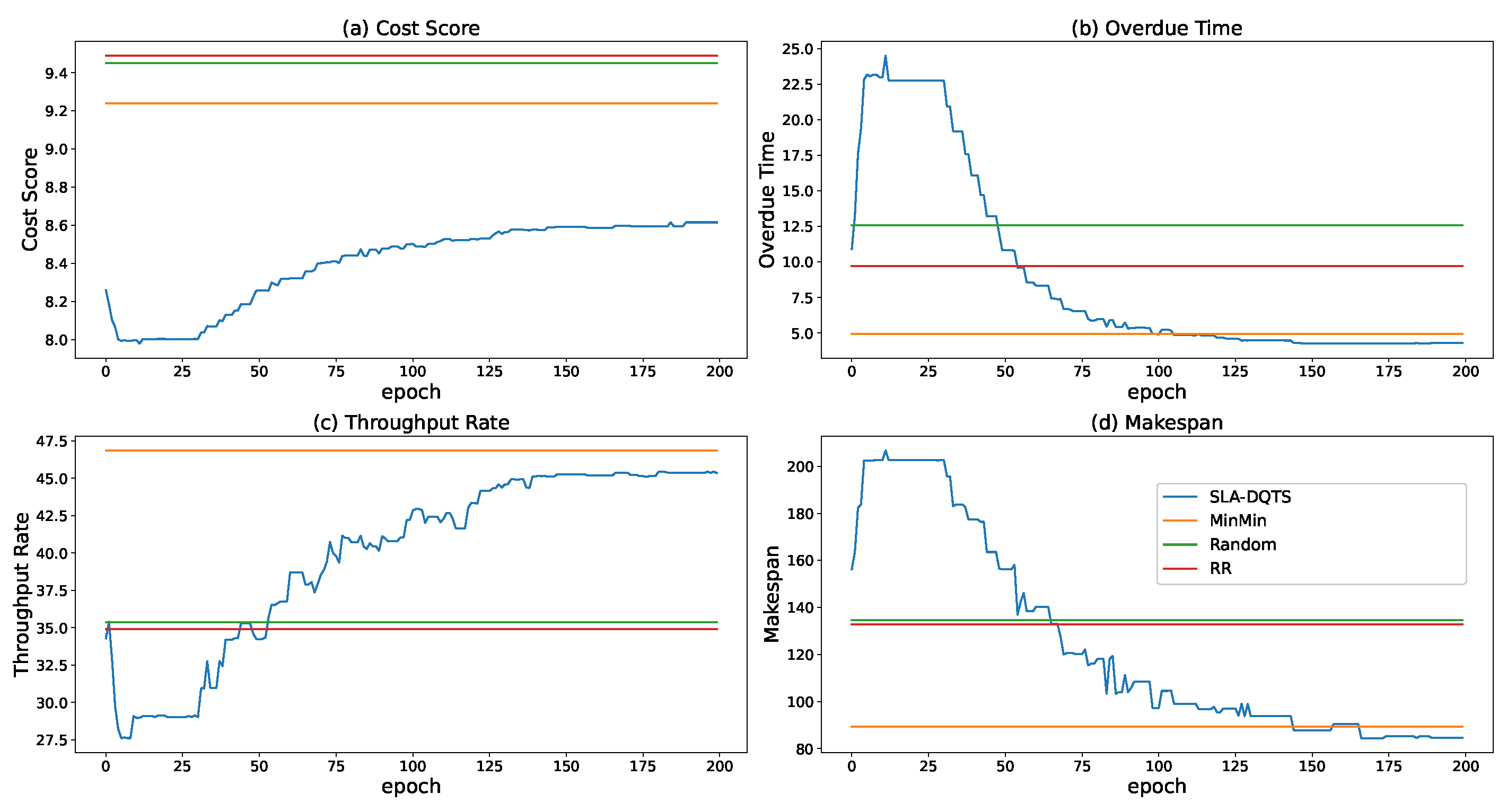
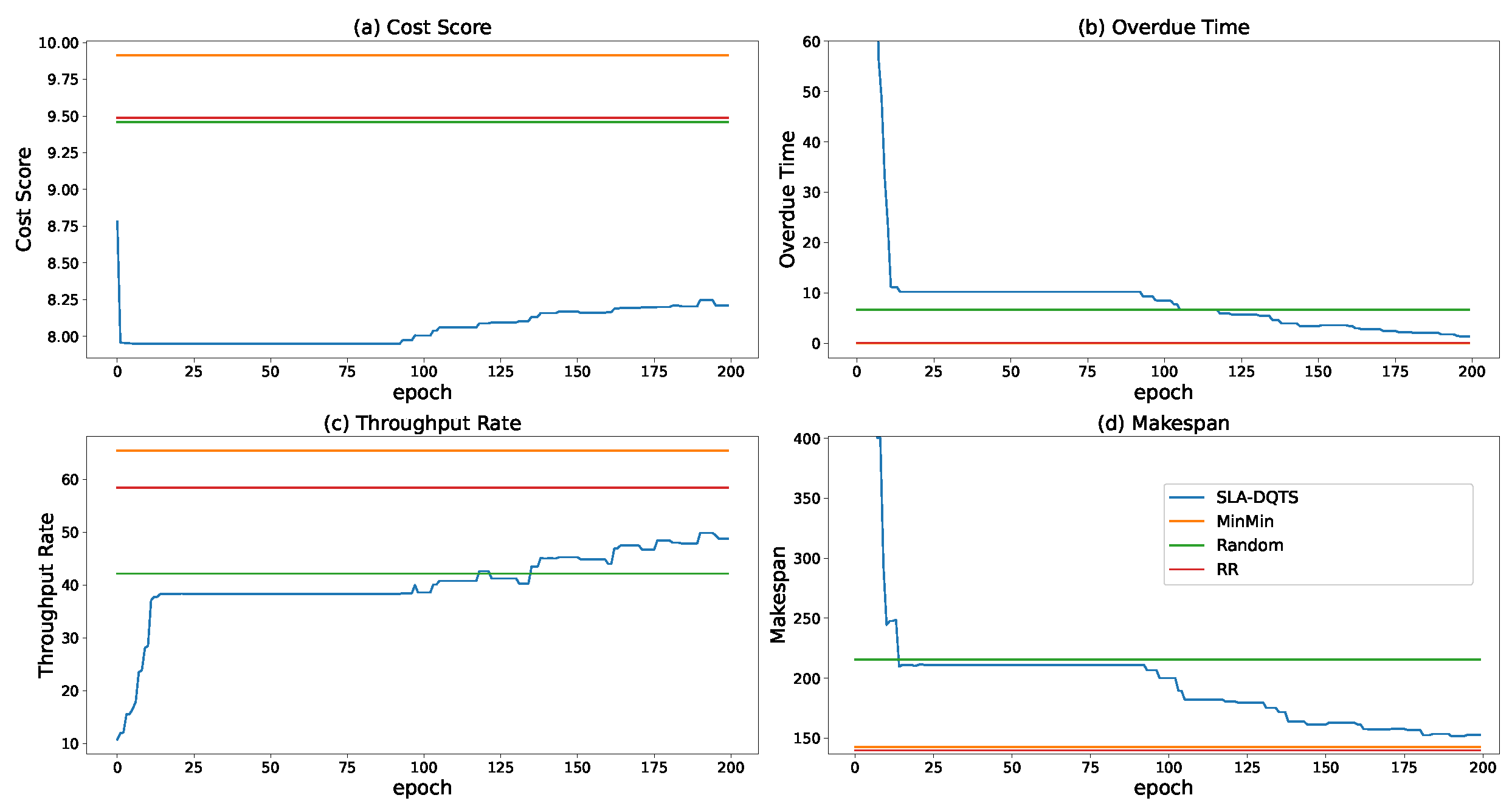
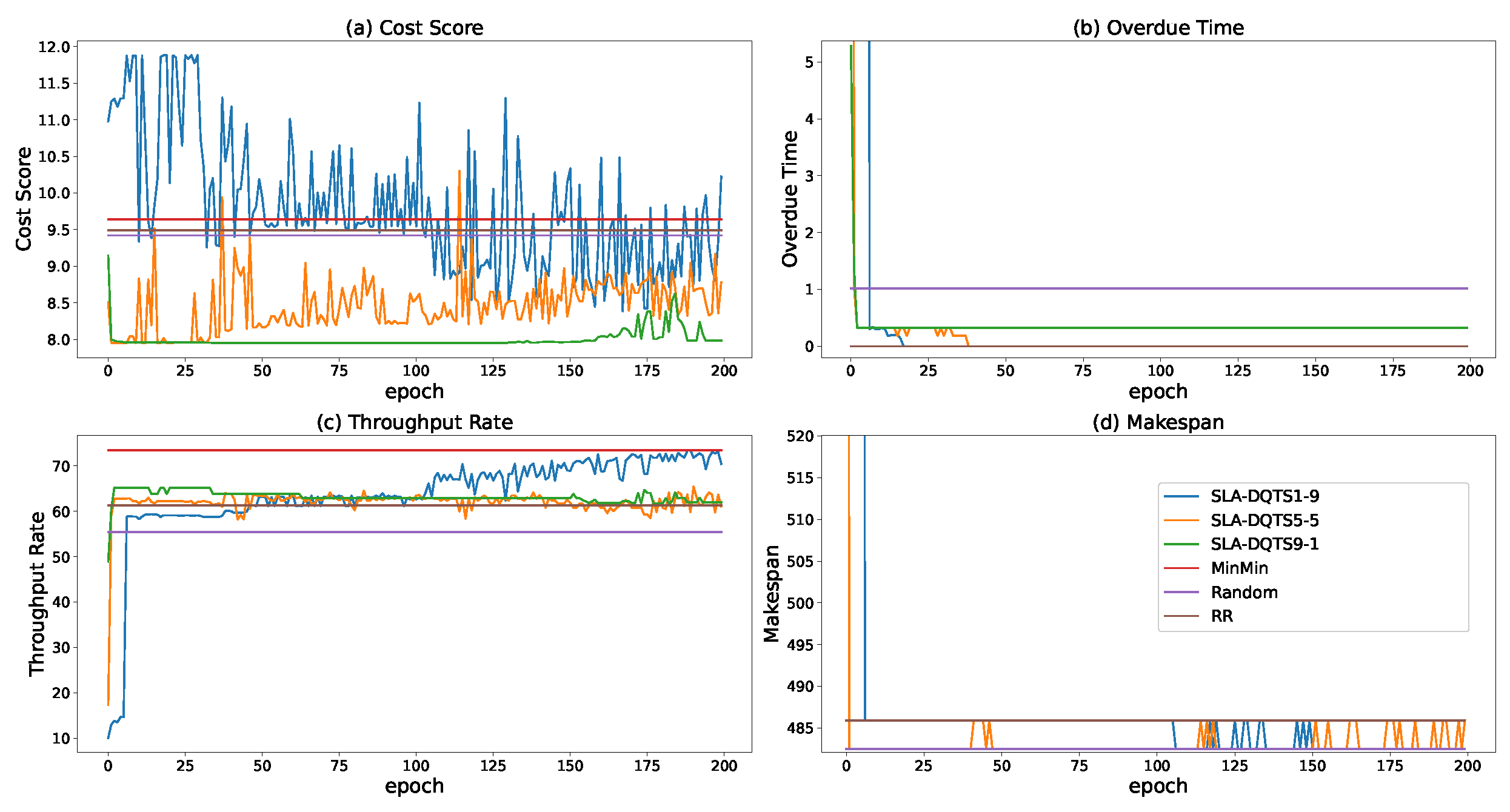
5. Performance Evaluation

We carried out experimental simulations to analyze the performance of our proposed scheme. We first introduce the design and evaluation objectives of the simulations. We compare it with existing scheduling algorithms designed in similar environments.

5.1. SETUP

To facilitate training and testing, based on the above modeling of the problem using CloudSim [37], an open-source toolkit for cloud computing, we used the Python language to build the simulation environment, assigning task scheduling to 54 VM instances.

The task was automatically generated by the program according to set parameters, and arrived in a Poisson distribution according to the set arrival rate. We simulate different loads by modifying the task reach speed in the simulation environment. Based on the phenomenon that human behavior conforms to the normative Poisson distribution to a certain extent, we use the Poisson distribution to calculate the user’s submission interval. Parameters include the number of tasks in each batch, task durations, resource requirements of tasks, and the lower limit and floating range. The relevant parameters of this experiment can be seen in

Table 2. Task generator parameters.

Parameter	Range
number	[2, 5)
mips	[100, 5100)
bw	[40, 290)
duration	[5, 35)

.

The three comparison algorithms were random (scheduling tasks to random clusters), round robin (scheduling tasks to different clusters by polling), and Min-Min (finding the task with the least load every time, and scheduling it to the earliest completed computing node). The performance indicators used in the evaluation are as follows.

• Makespan: completion time of the last task;
• Cost: the product of the execution time of each task and the price of the corresponding VM;
• Throughput: the sum of the task calculation and transmission amounts of each batch of tasks divided by the difference between the start and end times of the batch;
• Overdue time: the difference between the completion and loading times of each task compared with the expected completion time of the task. If it is less than the expected completion time, it is 0, and the difference if it is higher.

5.2. Experimental Results and Analysis

We compared the performance of the algorithm under three loads, taking the task arrival rate, i.e., $\lambda$ in the Poisson distribution, as the variable to control the load. The overdue time performance of the comparison function was used as a measure of the load level. Overdue times exceeding 1, in the range 0–1, and less than zero are regarded as high, medium, and low environmental loads, respectively. We believe that the optimization goal should depend on the load environment. In a high-load environment, user demand is high, and should be met first, i.e., the task should be completed within the expected completion time, and the timeout period should be minimized. In a medium-load environment, the task load and resource supply are balanced, user needs and costs are the main optimization goals, and the timeout period is allowed to fluctuate among values less than 1. In this article, users are set to have an insignificant perception of timeout periods less than 1. In a low-load environment, the resource supply far exceeds the task load, cost should be the main optimization goal, and high-cost VM usage should be reduced to maximize benefits.

High load: By modifying the task arrival rate to 1, the average overdue time of the comparison algorithm exceeds 1, indicating that the load is too high at this time, and the performance of the algorithm is tested. Figure 4 shows the changes in the evaluation indicators during training.

The overdue time under high load is greater than 1. According to the reward function (11), it can be seen that the reward is negative at this time. In the early stage, due to the fluctuation of the weights of exploration and early learning, the rate of return of the learning strategy decreases. With the increase in the number of learning samples, the model tends to be stable, and returns gradually increase. After the model converges, it can be seen that the algorithm in this paper has obvious advantages in cost and can minimize the overdue time. Since the Min-Min algorithm transfers the task to the VM that can complete it soonest, its throughput is dominant, and it can achieve excellent results in both timeout period and makespan. However, due to the lack of utilization of low-performance VMs, its cost is relatively high, and under high load, the timeout period and makespan cannot be optimized. Under high load, it can be clearly seen that task assignment to VMs has a greater impact on subsequent assignments, which reduces the fault tolerance rate. Therefore, the simple distribution methods of random and round robin perform poorly under high load.

Low load: By modifying the arrival rate to 0.05, the average overdue times of the comparison algorithms, except for the random algorithm, are 0. At this time, according to the reward function (11), the main source of reward is no longer overdue time, but cost and throughput. Three weight ratios are set to verify the function of the weight and performance of the algorithm under low load, with weights of 0.9–0.1, 0.5–0.5, and 0.1–0.9. The experimental results are shown in Figure 5.

As shown in Figure 5, in a low-load environment, the overdue time can easily converge to a target range of 0 or close to 0. According to the setting of the reward function, when the overdue time is less than 1, the proportion of the return comes from throughput, cost and overdue time, and the closer to 0, the larger the proportion of the first two items. SAL-DQTS9-1 takes cost as the main reward, so the use of more low-performance machines leads to low throughput and overdue tasks. Since the overdue time is close to zero, the penalty value is too small. The return from cost reduction can offset the corresponding penalty. The remaining two items tend to be balanced and have high throughput, so their overdue time converges to 0. From the comparison of the target curves of SAL-DQTS9-1 and SAL-DQTS1-9, the weight obviously has a certain influence on the effects of different indicators. A comparison with SAL-DQTS5-5 shows that in terms of cost, the convergence trend tends to the middle, while the throughput performance is similar to that of SAL-DQTS1-9. This is because the relationship between throughput and cost is not simple. After all, the cost is also related to time. Due to marginal effects, when the throughput is close to the maximum value, the throughput increase caused by the equal cost keeps dropping. At this time, the setting of the weight can make the optimization direction biased to the side with the higher weight. Moreover, the correction parameter ${\alpha }_r^1$, ${\alpha }_r^2$ in the reward functions (12) and (13) is set according to their respective maximum returns, so these two parameters constitute the upper limit of the return values under a single target similar. Moreover, the reward function curves of the two are not the same, so the weight cannot strictly make the optimization result and the weight ratio consistent. However, it is possible to modify the weight ratio to show the optimization tendency of a certain target. Through comparison, it can be seen that more balanced performance can be obtained in all aspects with a weight of 0.5–0.5. The advantage of the SAL-DQTS algorithm under low load is not obvious except in cost optimization. Min-Min will still adopt the earliest completion strategy under low load, so it will still tend to use high-performance VMs. Although the expiration time, throughput, and makespan are optimized, the cost increases accordingly. Under low load, there is no need to pursue such a high throughput rate and makespan. The appropriate sacrifice of some performance can still meet the demand and decrease the cost. Therefore, in the comparison function under low load, round robin has better overall performance.

Medium load: We modify the arrival rate to 0.2. At this time, the task overdue time under the comparison function scheduling is between 0 and 1, and the task load intensity is medium. Since the overdue time is less than one, according to the reward function (11), it can be seen that the return is affected by the trio of $r^1$, $r^2$, and $r^3$, and as the overdue gets closer to one the first two items become smaller. It can be seen from the low-load experiment that the weights of $r^1$ and $r^2$ are set to 0.5 and 0.5, respectively, so it is recommended to set this ratio in the medium-load experiment.

As shown in Figure 6, the overdue time of SAL-DQTS under moderate load and makespan is close to the optimal comparison algorithm. Although it is not as successful as Min-Min and round robin in throughput, it has obvious advantages in cost. Because it is a medium load, Min-Min has consistent performance with RR on overdue time and makespan, but because it prefers high-performance VMs to pursue higher throughput rates, the cost is higher than with RR. Under medium load, we believe that the performance supply is comparable to the task demand, and a small part of the response time and the makespan’s lower cost of zone change can be sacrificed within a certain range to achieve greater benefits. Based on this implementation, the comprehensive performance of RR is better than that of Min-Min.

Through the above three experiments, it can be seen that the proposed algorithm can dynamically adapt to changes of load in the environment and learn the corresponding strategies, meet user requirements as much as possible in the dynamic cloud environment, achieve excellent overdue time and makespan, and realize obvious advantages in task cost.

Complexity:

Table 3. Algorithm complexity.

Algorithm	Flops	Memory	Complexity	Execution Time
SLA_DQTS	N*247 k	124 k	247 k	0.01362
Min-Min	-	1	N*M	0.00477
Random	-	1	1	0.00296
RR	-	1	1	0.00165

shows the relevant indicators of the complexity of the algorithm, including the flops [38], memory, time complexity, and simulation execution time. Due to the model structure, the calculation amount is proportional to the number of VMs, which is $N\ast 247 \mathrm{kFlops}$, where N is the number of VMs. This process is parallel, so the calculation time is not linear with the number of VMs, and the time complexity is 247 k. The Min-Min needs to select the smallest task and the earliest completed VM, so the complexity is $N\ast M$, and M is the number of tasks. The Random and RR algorithms only use random and polling methods, respectively, so their complexity is 1. The last column in the table is the scheduling time of a single task of each comparison algorithm in the simulation environment. It can be seen that SLA_DQTS is significantly higher than the comparison algorithm. Although the training and decision making of the model can be asynchronous, compared with the traditional heuristic algorithm, deep reinforcement learning requires additional training costs and cannot be ignored.

6. Conclusions

In tackling the online task scheduling problem with SLA constraints, an artificial intelligence scheduling algorithm based on DDQN was proposed, using a Gaussian distribution of relevant features as input to make the input vector dimension of the model fixed to adapt to the change in the number of VMs. The reward function uses the throughput rate, expense rate, and average overdue time as the main components of the return. Considering the user experience, a reward function with average overdue time as the main optimization objective was proposed to adapt to the change of load in the cloud environment. We used the average overdue time as a standard to measure different loads and evaluate the performance of the algorithm under different loads through simulations. Our method involved shorter task overdue times and lower costs under SLA constraints, and could be adapted to cloud computing in different load environments.

In a large-scale task scheduling problem, the complexity will inevitably increase with the increase of the problem size, and it is extremely resource-intensive to train each model from zero. In the future, we plan to expand and improve our solutions in terms of hierarchical scheduling and migration learning to cope with large-scale online task scheduling in cloud computing, and to enable it to learn more quickly.

References

1. Kumar, K.; Hans, A.; Sharma, A.; Singh, N. Towards the various cloud computing scheduling concerns: A review. In Proceedings of the 2014 Innovative Applications of Computational Intelligence on Power, Energy and Controls with Their Impact on Humanity (CIPECH), Ghaziabad, India, 28–29 November 2014; pp. 482–485. [Google Scholar]
2. Ran, L.; Shi, X.; Shang, M. SLAs-aware online task scheduling based on deep reinforcement learning method in cloud environment. In Proceedings of the 2019 IEEE 21st International Conference on High Performance Computing and Communications, IEEE 17th International Conference on Smart City, IEEE 5th International Conference on Data Science and Systems (HPCC/SmartCity/DSS), Zhangjiajie, China, 10–12 August 2019; pp. 1518–1525. [Google Scholar]
3. Keivani, A.; Tapamo, J.R. Task Scheduling in Cloud Computing: A Review. In Proceedings of the 2019 International Conference on Advances in Big Data, Computing and Data Communication Systems (icABCD), Winterton, South Africa, 5–6 August 2019; pp. 1–6. [Google Scholar]
4. Almansour, N.; Allah, N.M. A Survey of Scheduling Algorithms in Cloud Computing. In Proceedings of the 2019 International Conference on Computer and Information Sciences (ICCIS), Chengdu, China, 2–3 November 2019; pp. 11–18. [Google Scholar]
5. Ma, Y.; Yang, L.; Hu, F. Research on a cloud resource scheduling strategy based on asynchronous reinforcement learning. In Proceedings of the 2021 IEEE International Conference on Power Electronics, Computer Applications (ICPECA), Shenyang, China, 22–24 January 2021; pp. 920–923. [Google Scholar]
6. Van Hasselt, H.; Guez, A.; Silver, D. Deep reinforcement learning with double q-learning. In Proceedings of the AAAI Conference on Artificial Intelligence, Phoenix, AZ, USA, 12–17 February 2016; Volume 30. [Google Scholar]
7. Shen, W. Distributed manufacturing scheduling using intelligent agents. IEEE Intell. Syst. 2002, 17, 88–94. [Google Scholar] [CrossRef]
8. Singh, P.; Dutta, M.; Aggarwal, N. A review of task scheduling based on meta-heuristics approach in cloud computing. Knowl. Inf. Syst. 2017, 52, 1–51. [Google Scholar] [CrossRef]
9. Patil, N.; Aeloor, D. A review-different scheduling algorithms in cloud computing environment. In Proceedings of the 2017 11th International Conference on Intelligent Systems and Control (ISCO), Tamilnadu, India, 5–6 January 2017; pp. 182–185. [Google Scholar]
10. Pan, Y.; Wang, S.; Wu, L.; Xia, Y.; Zheng, W.; Pang, S.; Zeng, Z.; Chen, P.; Li, Y. A Novel Approach to Scheduling Workflows upon Cloud Resources with Fluctuating Performance. Mobile Netw. Appl. 2020, 25, 690–700. [Google Scholar] [CrossRef]
11. Mboula, J.E.N.; Kamla, V.C.; Djamegni, C.T. Cost-time trade-off efficient workflow scheduling in cloud. Simul. Model. Pract. Theory 2020, 103, 102107. [Google Scholar] [CrossRef]
12. Zhao, C.; Wang, J. Dynamic Workflow Scheduling based on Autonomic Fault-Tolerant Scheme Selection in Uncertain Cloud Environment. In Proceedings of the 2020 6th International Symposium on System and Software Reliability (ISSSR), Chengdu, China, 24–25 October 2020; pp. 38–45. [Google Scholar]
13. Lin, B.; Guo, W.; Lin, X. Online optimization scheduling for scientific workflows with deadline constraint on hybrid clouds. Concurr. Comput. Pract. Exp. 2016, 28, 3079–3095. [Google Scholar] [CrossRef]
14. Rodriguez, M.A.; Buyya, R. Deadline based resource provisioningand scheduling algorithm for scientific workflows on clouds. IEEE Trans. Cloud Comput. 2014, 2, 222–235. [Google Scholar] [CrossRef] [Green Version]
15. Chen, H.; Guo, W. Real-time task scheduling algorithm for cloud computing based on particle swarm optimization. In Proceedings of the Second International Conference on Cloud Computing and Big Data in Asia, Huangshan, China, 17–19 June 2015; pp. 141–152. [Google Scholar]
16. Chen, X.; Long, D. Task scheduling of cloud computing using integrated particle swarm algorithm and ant colony algorithm. Clust. Comput. 2019, 22, 2761–2769. [Google Scholar] [CrossRef]
17. Hall, J.; Moessner, K.; Mackenzie, R.; Carrez, F.; Foh, C.H. Dynamic Scheduler Management Using Deep Learning. IEEE Trans. Cogn. Commun. Netw. 2020, 6, 575–585. [Google Scholar] [CrossRef] [Green Version]
18. Al-Zoubi, H. Efficient Task Scheduling for Applications on Clouds. In Proceedings of the 2019 6th IEEE International Conference on Cyber Security and Cloud Computing (CSCloud)/2019 5th IEEE International Conference on Edge Computing and Scalable Cloud (EdgeCom), Paris, France, 21–23 June 2019; IEEE: New York, NY, USA, 2019; pp. 10–13. [Google Scholar]
19. Reddy, G.N.; Kumar, S.P. Regressive Whale Optimization for Workflow Scheduling in Cloud Computing. Int. J. Comput. Intell. Appl. 2019, 18, 1950024. [Google Scholar] [CrossRef]
20. Khodar, A.; Chernenkaya, L.V.; Alkhayat, I.; Al-Afare, H.A.F.; Desyatirikova, E.N. Design Model to Improve Task Scheduling in Cloud Computing Based on Particle Swarm Optimization. In Proceedings of the 2020 IEEE Conference of Russian Young Researchers in Electrical and Electronic Engineering (EIConRus), Saint Petersburg, Russia, 27–30 January 2020; pp. 345–350. [Google Scholar]
21. Zhou, Z.; Chang, J.; Hu, Z.; Yu, J.; Li, F. A modified PSO algorithm for task scheduling optimization in cloud computing. Concurr. Comput. Pract. Exp. 2018, 30, e4970. [Google Scholar] [CrossRef]
22. Chen, J.; Han, P.; Liu, Y.; Du, X. Scheduling independent tasks in cloud environment based on modified differential evolution. Concurr. Comput. Pract. Exp. 2021. [Google Scholar] [CrossRef]
23. Barrett, E.; Howley, E.; Duggan, J. A learning architecture for scheduling workflow applications in the cloud. In Proceedings of the 2011 IEEE Ninth European Conference on Web Services, Lugano, Switzerland, 14–16 September 2011; pp. 83–90. [Google Scholar]
24. Peng, Z.; Cui, D.; Zuo, J.; Li, Q.; Xu, B.; Lin, W. Random task scheduling scheme based on reinforcement learning in cloud computing. Clust. Comput. 2015, 18, 1595–1607. [Google Scholar] [CrossRef]
25. Xiao, Z.; Liang, P.; Tong, Z.; Li, K.; Khan, S.U.; Li, K. Self-adaptation and mutual adaptation for distributed scheduling in benevolent clouds. Concurr. Comput. Pract. Exp. 2017, 29, e3939. [Google Scholar] [CrossRef]
26. Soualhia, M.; Khomh, F.; Tahar, S. A dynamic and failure-aware task scheduling framework for hadoop. IEEE Trans. Cloud Comput. 2018, 8, 553–569. [Google Scholar] [CrossRef]
27. Riera, J.F.; Batallé, J.; Bonnet, J.; Días, M.; McGrath, M.; Petralia, G.; Liberati, F.; Giuseppi, A.; Pietrabissa, A.; Ceselli, A.; et al. TeNOR: Steps towards an orchestration platform for multi-PoP NFV deployment. In Proceedings of the 2016 IEEE NetSoft Conference and Workshops (NetSoft), Seoul, Korea, 6–10 June 2016; pp. 243–250. [Google Scholar]
28. Jayswal, A.K. Hybrid Load-Balanced Scheduling in Scalable Cloud Environment. Int. J. Inf. Syst. Model. Des. (IJISMD) 2020, 11, 62–78. [Google Scholar] [CrossRef]
29. Kaur, A.; Singh, P.; Singh Batth, R.; Peng Lim, C. Deep-Q learning-based heterogeneous earliest finish time scheduling algorithm for scientific workflows in cloud. Software Pract. Exp. 2020. [Google Scholar] [CrossRef]
30. Cui, D.; Peng, Z.; Xiong, J.; Xu, B.; Lin, W. A reinforcement learning-based mixed job scheduler scheme for grid or iaas cloud. IEEE Trans. Cloud Comput. 2017, 8, 1030–1039. [Google Scholar] [CrossRef]
31. Tong, Z.; Chen, H.; Deng, X.; Li, K.; Li, K. A scheduling scheme in the cloud computing environment using deep Q-learning. Inf. Sci. 2020, 512, 1170–1191. [Google Scholar] [CrossRef]
32. Li, F.; Hu, B. Deepjs: Job scheduling based on deep reinforcement learning in cloud data center. In Proceedings of the 2019 4th International Conference on Big Data and Computing, Guangzhou, China, 10–12 May 2019; pp. 48–53. [Google Scholar]
33. Dong, T.; Xue, F.; Xiao, C.; Li, J. Task scheduling based on deep reinforcement learning in a cloud manufacturing environment. Concurr. Comput. Pract. Exp. 2020, 32, e5654. [Google Scholar] [CrossRef]
34. Liu, N.; Li, Z.; Xu, J.; Xu, Z.; Lin, S.; Qiu, Q.; Tang, J.; Wang, Y. A hierarchical framework of cloud resource allocation and power management using deep reinforcement learning. In Proceedings of the 2017 IEEE 37th International Conference on Distributed Computing Systems (ICDCS), Atlanta, GA, USA, 5–8 June 2017; pp. 372–382. [Google Scholar]
35. Sutton, R.S.; Barto, A.G. Reinforcement Learning: An Introduction; MIT Press: Cambridge, MA, USA, 2018. [Google Scholar]
36. Armbrust, M.; Fox, A.; Griffith, R.; Joseph, A.D.; Katz, R.H.; Konwinski, A.; Lee, G.; Patterson, D.A.; Rabkin, A.; Stoica, I.; et al. Above the Clouds: A Berkeley View of Cloud Computing; Technical Report UCB/EECS-2009-28; EECS Department, University of California: Berkeley, CA, USA, 2009; Volume 28. [Google Scholar]
37. Calheiros, R.N.; Ranjan, R.; Beloglazov, A.; De Rose, C.A.; Buyya, R. CloudSim: A toolkit for modeling and simulation of cloud computing environments and evaluation of resource provisioning algorithms. Softw. Pract. Exp. 2011, 41, 23–50. [Google Scholar] [CrossRef]
38. Molchanov, P.; Tyree, S.; Karras, T.; Aila, T.; Kautz, J. Pruning convolutional neural networks for resource efficient inference. arXiv 2016, arXiv:1611.06440. [Google Scholar]
Figure 1. Reinforcement learning paradigm.
Applsci 11 09360 g001
Figure 2. Task scheduling framework.
Applsci 11 09360 g002
Figure 3. Q value mode (a) S Q ( s , a n ) mode, (b) S , a Q ( a ) mode.
Applsci 11 09360 g003
Figure 4. Performance of SAL-DQTS algorithm and comparison algorithms under high-load environment.
Applsci 11 09360 g004
Figure 5. Performance of SAL-DQTS algorithm with different weights and comparison algorithm in a low-load environment.
Applsci 11 09360 g005
Figure 6. Performance of SAL-DQTS and comparison algorithms under medium-load environment.
Applsci 11 09360 g006