Concrete Crack Detection Based on Well-Known Feature Extractor Model and the YOLO_v2 Network

Abstract

This paper compares the crack detection performance (in terms of precision and computational cost) of the YOLO_v2 using 11 feature extractors, which provides a base for realizing fast and accurate crack detection on concrete structures. Cracks on concrete structures are an important indicator for assessing their durability and safety, and real-time crack detection is an essential task in structural maintenance. The object detection algorithm, especially the YOLO series network, has significant potential in crack detection, while the feature extractor is the most important component of the YOLO_v2. Hence, this paper employs 11 well-known CNN models as the feature extractor of the YOLO_v2 for crack detection. The results confirm that a different feature extractor model of the YOLO_v2 network leads to a different detection result, among which the AP value is 0.89, 0, and 0 for ‘resnet18’, ‘alexnet’, and ‘vgg16’, respectively meanwhile, the ‘googlenet’ (AP = 0.84) and ‘mobilenetv2’ (AP = 0.87) also demonstrate comparable AP values. In terms of computing speed, the ‘alexnet’ takes the least computational time, the ‘squeezenet’ and ‘resnet18’ are ranked second and third respectively; therefore, the ‘resnet18’ is the best feature extractor model in terms of precision and computational cost. Additionally, through the parametric study (influence on detection results of the training epoch, feature extraction layer, and testing image size), the associated parameters indeed have an impact on the detection results. It is demonstrated that: excellent crack detection results can be achieved by the YOLO_v2 detector, in which an appropriate feature extractor model, training epoch, feature extraction layer, and testing image size play an important role.

1. Introduction

Timely detection of cracks in concrete structures is an important step of structural health monitoring (SHM) [1]. In recent years, due to aging and environmental impacts, surface cracks of infrastructures, especially concrete structures, are a hidden danger that needs to be focused on [2]. Therefore, it is necessary to detect the cracks of concrete structures to prevent any further losses in their durability. In general, inspectors collect images or videos through on-site optical instruments, process the collected data, and finally draw the inspection conclusions; this is an effective method for simple tasks, but it is unsuitable for large-scale inspection due to its low efficiency and high cost [3]. The detection of bridge surface defects based on images is highly repetitive work [4]. In the case of a large amount of data, manual detection is tedious, inefficient, and expensive [5]. Therefore, it is essential to investigate some automated methods, e.g., artificial intelligence (AI) technology, to undertake this labor-intensive work.

AI technology provides a more advanced method for SHM, which has the ability to perform various tasks (such as classification or regression) with outstanding performance. A number of AI-based image processing methods can be used for bridge defect detection [5,6]. Fujita et al. detected cracks in an asphalt pavement surface using a support vector machine (SVM); Shi et al. detected road cracks using random structured forests (RSF) [7]. Furthermore, as an emerging AI algorithm, the artificial neural network (ANN) [8] has been used to classify rail surface cracks [9], and detect potholes on an asphalt pavement surface [10], which has become a popular technique in the SHM field. However, the practical application of this method is limited due to its slow convergence, over-fitting, and high computational cost, etc. [11]. Therefore, a fast and automatic feature extraction algorithm [12,13] is needed to process the huge monitoring data [12].

The application of deep convolutional neural network (DCNN) algorithms further improve the detection method, and can automatically extract features from the raw data and gradually obtain advanced features through multiple processing layers [14]. In the field of SHM, the CNN can extract the signal distribution features from the images of fused time and frequency domain information [15], extract the frequency features from the acceleration signals [12], and extract the structural damage features from the modal shapes [13]. Meanwhile, a DCNN uses partial connections and pooling of neurons, thus, requires less computation, has better robustness, which makes the DCNN an effective and fast SHM method. A lot of research has been conducted for SHM based on the DCNN [16,17] by using vibration signals [12,18,19] and defect images [16,20,21]. In the field of defect images-based SHM [22], image classification is a popular method for automatic defect detection. The DCNN has been used in image classification for pavement cracks [23,24], sewer defects [21], and road damages [25]. In further research to determine the location of defects, a basic method was proposed to scan the image with a fixed size sliding window and then apply the trained DCNN to each small window. With this method, Cha et al. proposed a DCNN model to classify whether there are concrete cracks in each image block [16]. Liang et al. employed a transfer learning model (‘vgg-16’) [26] to classify two types of defects: cracking and spalling [27]. These studies confirmed that the location of cracks in an image can be obtained by using a sliding window. However, the challenge of this sliding window method is to find the appropriate window size when dealing with defects of different scales. Moreover, the computational cost of this method is very high, because the DCNN classifier must be applied to every window in every image many times. To improve the efficiency of detecting and locating an object (such as a crack), more advanced object detection technology needs to be further explored.

Region-based classification or object detection provides a state-of-the-art method for SHM. This method creates a bounding box around the region of interest (ROI), such as cracks, spalls, components, etc. Common methods include two-stage and one-stage algorithms. Two-stage algorithms include region-based CNN (R-CNN), Fast R-CNN, and Faster R-CNN. The R-CNN has been applied to post-event building reconnaissance with an accuracy of nearly 60% [28], and the related research shows that its computation speed is low [29]. As an advanced version of the R-CNN, the Fast R-CNN is proposed to improve computational efficiency and accuracy, and it is used to detect different defects and locations of concrete structures [30]. Then a faster R-CNN (Faster R-CNN) is proposed by introducing a region proposal network (RPN) [29], and it is employed to automatically detect structural components of the RC bridge system [31] and cracks for asphalt pavements [32]. Although the above studies demonstrated the ideal accuracy of two-stage detectors, their detection is not very fast. High-speed detection is essential for the development of real-time automatic inspection systems, which seem to be the future trend of the industry [33]. Due to the above limitations, one-stage detectors have been proposed. The popular one-stage models include You Only Look Once (YOLO) and single-shot multi-box detector (SSD). These are faster than two-stage deep learning object detectors, such as region-based CNN (i.e., Faster R-CNN) [34]. Recent studies employed the YOLO network to detect multiple concrete bridge defects [6] and pavement cracks [35]; the SSD was also applied to detect road defects in real-time [25]. However, some researchers found that locating defects using one-stage detectors could compromise the accuracy of the detection [36]. The above research results show that the crack detection method based on an object detection algorithm has become a hot topic, and both two-stage and one-stage algorithms need a feature extractor (i.e., a CNN model), but the effect of different feature extractors on image feature extraction is not clear. With the continuous updating of neural networks, some well-known CNN models are widely used to complete different situations, which will provide more suitable feature extractors for defect detection. Therefore, the influence of different feature extractors on crack detection is a problem worthy of in-depth investigation.

The application of transfer learning technology provides a state-of-the-art method for feature extraction. As the well-known CNN models have strong feature extraction ability, it will save a lot of time (no-training process) to use these CNN models as feature extractors. Therefore, this paper compares various CNN models (e.g., ‘alexnet’, ‘resnet18’, etc.) as the feature extractor of the YOLO_v2 to identify a model with high precision and fast computational speed. Meanwhile, parametric studies are implemented to confirm the effect of the relevant parameters on the detection results. Finally, the influence of different feature layers on the detection results is revealed by feature visualization.

2. Methods

Popular programming languages such as Java, C++, Python, and MATLAB (MathWorks Inc., Natick, MA, USA) are usually used to build the YOLO_v2, among which MATLAB is more suitable for non-professional programmers. In this paper, the YOLO_v2 was established by using MATLAB, in which 11 CNN models were used respectively as the feature extractor of the YOLO_v2 network. The precision and computational cost were compared by using different feature extractors.

2.1. YOLO_v2

The YOLO_v2 object detector is a one-stage detection network, which runs a CNN model (Figure 1) on an input image to produce feature images from a feature extraction layer. Then, these feature images are input into the YOLO_v2 detection layer and the classification and anchor box of the detection object are obtained. Therefore, the selection of the feature extractor model would be an interesting focus for object detection. It should be noted that the detailed feature extractor contains the convolution, pooling, and ReLU layers [18].

Furthermore, anchor boxes (Figure 2) were adopted to detect classes of objects in the image. Anchor boxes are a set of predefined bounding boxes of certain heights and widths. These boxes (defined based on the object sizes of the samples) capture the scale and aspect ratio of the specific object classes to be detected. The use of anchor boxes significantly improves the efficiency of object detection [37], making real-time detection possible.

For the detection layer, the YOLO_v2 predicted the location of the anchor box by the following four steps (Figure 2):

• Step 1: Obtained feature images from the feature extractor;
• Step 2: The predefined anchor boxes were tiled across the image;
• Step 3: To generate the final object detections, tiled anchor boxes that belonged to the background class were removed;
• Step 4: The location error (the distance between refined and predefined anchor box) was gradually reduced by minimizing the loss function. As shown in Figure 2, the upper left coordinates of the predefined anchor box were (x₁, y₁), and the refined anchor box was (x₂, y₂). During training, the precise location of the anchor box was obtained by minimizing the loss function (squared error loss, SEL):

  $$SEL={(x_2-x_1)}^2+{(y_2-y_1)}^2$$

  (1)

Finally, the most suitable anchor box (crack location) and the highest classification score (crack or background) were obtained. As a result, the YOLO_v2 predicted the class probability (i.e., how precisely the model found the object) and the crack location (i.e., using anchor box) for each image.

2.2. Transfer Learning-Based Feature Extractors

Transfer learning technology is the reuse of a pre-trained model on a new problem. With transfer learning technology, we transferred the weights that CNN had learned at ‘Question A’ to a new ‘Question B’. Some well-known CNN models (e.g., alexnet, googlenet, etc.) were trained on the ImageNet database [22] which was used in the ImageNet Large-Scale Visual Recognition Challenge (ILSVRC) [38]. These CNN models had strong feature extraction ability and could classify images into 1000 object categories. Therefore, we employed these excellent CNN models as feature extractors of the YOLO_v2.

In this paper, 11 well-known CNN models were employed as the YOLO_v2 feature extractor. including: ‘alexnet’, ‘googlenet’, ‘mobilenetv2’, ‘inceptionv3’, ‘squeezenet’, ‘resnet18’, ‘resnet50’, ‘resnet101’, ‘vgg16’, ‘vgg19’, and ‘inceptionresnetv2’, which were named as TN1, TN2, …, TN11, respectively.

Table 1. The properties of these well-known convolutional neural network (CNN) models.

Network	TN1	TN2	TN3	TN4	TN5	TN6	TN7	TN8	TN9	TN10	TN11
Depth (layers)	8	22	53	48	18	18	50	101	16	19	164
Model size (MB)	227	27	13	89	4.6	44	96	167	515	535	209

lists their properties;

Table 2. The feature extraction layer of these well-known CNN models [39].

Network	Feature Extraction Layer	Network	Feature Extraction Layer
TN1	‘relu5’	TN7	‘activation_40_relu’
TN2	‘inception_4d-output’	TN8	‘res4b22_relu’
TN3	‘block_13_expand_relu’	TN9	‘relu5_3’
TN4	‘mixed7’	TN10	‘relu5_4’
TN5	‘fire5-concat’	TN11	‘block17_20_ac’
TN6	‘res4b_relu’

lists the feature extraction layer of these well-known CNN models, the details are referred to in the manual of the MATLAB [39]. The network included a series of processing layers, e.g., convolutional layer, pooling layer, fully connected layer, etc. RGB (three channels) images were used as the input for all networks.

2.3. Experimental Setup and Performance Evaluation

An image dataset included 990 RGB crack images (namely CR, 227 × 227 pixels) of a concrete bridge. Among them, 90% of the images were used for training (891 images) and 10% for testing (99 images) the performance of the YOLO_v2. The ‘Image labeler’ toolbox in MATLAB was employed to label cracks (including the classification and location of cracks with anchor boxes). Figure 3 shows two examples of the labeled images. The YOLO_v2 was built using Deep Learning Toolbox in MATLAB. The specific parameters included: (1) Optimizer: sgdm [40]; (2) Mini-batch-size: 8; (3) Maximum epoch: 30; (4) Learning rate: 0.001. The training platform was performed on a computer with NVIDIA GTX GeForce 1650 GPU, Intel Core i7-4790 @ 3.60 GHz CPU, windows 10.

The performance of the YOLO_v2 was investigated by comparing four factors:

(1) Feature extractor model. The 11 well-known CNN models (illustrated in Section 2.2) were used as the feature extractor of the YOLO_v2;

(2) Maximum epoch. An epoch was a full circle in the entire training dataset. When the precision of the YOLO_v2 reached a plateau and was clearly no longer improving, the starting epoch of the plateau was defined as the maximum epoch. In this paper, 1~30 epochs were designed to observe the change of detection results with epochs.

(3) Feature images in different CNN layers. The optimal model obtained in Step (2) was the feature extractor, and feature images of multiple layers were obtained and used as the input of the YOLO_v2 detection layer, the influence of feature images of different layers on the detection results was studied.

(4) Testing image size. On the basis of Step (3), different sized (32 × 32, 64 × 64, 128 × 128, 256 × 256, 512 × 512, 1024 × 1024, 2048 × 2048) images were used as the testing data. The influence of testing image size on detection results was studied.

Computational cost and detection precision are important indexes to evaluate the performance of the YOLO detector. The computation time (the unit is seconds) was the processing time of the entire detection process, which included feature extraction and detector training. Detection precision included precision, recall, and average precision (AP). The following is a detailed explanation of these three terms:

Precision: represented the classification effect of the classifier, which was the ratio of true positive instances to the total positive instances (Equation (2)). Recall: was a ratio of true positive instances to the sum of true positives and false negatives in the detection (Equation (3)).

$$P=\frac{TP}{TP+FP}$$

(2)

$$R=\frac{TP}{TP+FN}$$

(3)

where TP (true positive instances): positive instances that were predicted to be positive instances. FN (false negative instances): positive instances that were predicted to be negative instances. FP (false positive instances): negative instances that were predicted to be positive instances.

AP was used to reflect the detection precision, which was a combined outcome of the precision and recall metrics.

$$AP={\displaystyle \sum _{k=1}^{N}P(k)\Delta R(k)}$$

(4)

where k = 1, 2, …, N; and N is the number of samples, P(k) is the precision of the k-th sample, and is the difference of $\Delta R(k)$ the recall between the k-th sample and k − 1-th sample.

3. Results and Discussion

3.1. Crack Detection Results of the YOLO_v2

The testing images described in Section 2.3 were input into the trained YOLO_v2, the detection results of using 11 CNN models as the feature extractors are illustrated in

Table 3. The results of different feature extractors in locating cracks.

Models	Detection Precision (AP)	Computational Cost (s)
alexnet	0	2,266
googlenet	0.84	4,451
mobilenetv2	0.87	8,763
inceptionv3	0.16	9,720
squeezenet	0.60	2,873
resnet18	0.89	3,299
resnet50	0.02	10,321
resnet101	0.73	17,457
vgg16	0	13,580
vgg19	0.23	15,719
inceptionresnetv2	0.86	22,523

. The feature extractor based on six transfer learning models achieved superior detection results, the AP values were higher than 0.6. Among them, ‘resnet18’ achieved the best detection results with the AP value reaching 0.89, and ‘googlenet’ (AP = 0.84) and ‘mobilenetv2’ (AP = 0.87) also had comparable AP values. The performance of some feature extractors (i.e., ‘alexnet’, ‘resnet50’, ‘vgg16’) was unsatisfactory, and the AP value tended to 0.

The computational cost was an important index to evaluate whether the model was suitable for fast and real-time detection. In this paper, the computation time of the 11 models was recorded and illustrated in Table 3. The ‘alexnet’ took the least computation time, the ‘squeezenet’ and ‘resnet18’ were ranked second and third respectively in terms of the computation time; the ‘inceptionresnetv2’ used the most computation time which was more than 10 times that of ‘alexnet’. For a certain series of networks, the computational cost would increase with the increase of network complexity, e.g., in the series of ‘resnet18’, resnet50’, and ‘resnet101’. On the whole, ‘resnet18’ was the best detector in the trade-off between detection precision and computational cost.

3.2. Parametric Study

Three parameters of the YOLO_v2 using ‘resnet18’ (as the feature extractor) were studied, (1) Influence of the training epochs on detection results; (2) Influence of the feature extraction layer on detection results; (3) Influence of the testing image size on detection results.

(1) A case study for the maximum epoch was therefore performed on a training set with 891 training images to determine the optimal epoch for the training. The AP value and computing time were recorded in Figure 4, 22–30 epochs corresponded to the most stable AP value, meanwhile, the computational cost increased with the increase of the epoch number. Therefore, an optimal epoch of 22 was chosen for the best balance between speed and precision.

By studying the influence of epoch on detection results, the optimal detection precision could be achieved with fewer epochs. Because once the detection precision was stable, with the increase of epoch number, the computational cost would increase, which was not necessary.

(2) Eight layers (L1~L8 in Figure 5) of the ‘resnet18’ were employed as the feature extraction layers of the YOLO_v2 respectively. These networks were trained with the training data, the computational cost was recorded, and then the testing data were input into the eight YOLO_v2 detectors. The results are illustrated in

Table 4. The detection results of different feature extraction layers (‘resnet18’).

Layers	Detection Precision (AP)	Computational Cost (s)
L1	0.18	2411
L2	0.40	2558
L3	0.82	2637
L4	0.80	2767
L5	0.86	2944
L6	0.89	3299
L7	0.87	3739
L8	0	4155

. The AP value increased first, and then decreased with the increase of the layer depth; ‘L6’ achieved the best detection results. However, the computational time increased gradually by selecting a deeper layer as the feature extraction layer.

(3) According to the optimal network obtained above (the YOLO_v2 with ‘resnet18’, and ‘L6’ as the feature extraction layer), seven testing image sets (Section 2.3) with different sizes were input into the YOLO_v2 respectively to evaluate the influence of image resolution (image size) on detection results (

Table 5. Detection results of different sizes of testing images.

Image Size	Detection Precision (AP)	FPS
32 × 32	0	20
64 × 64	0.15	17
128 × 128	0.81	14
256 × 256	0.88	13
512 × 512	0.88	11
1024 × 1024	0.89	10
2048 × 2048	0.88	5

). The results indicated that: with the increase of resolution, the AP value increased gradually and tended to become stable. However, The FPS (frames per second), which evaluates the testing speed, decreased gradually with the increase of resolution. Therefore, the image with an appropriate resolution could achieve the optimal combination of precision and computing speed.

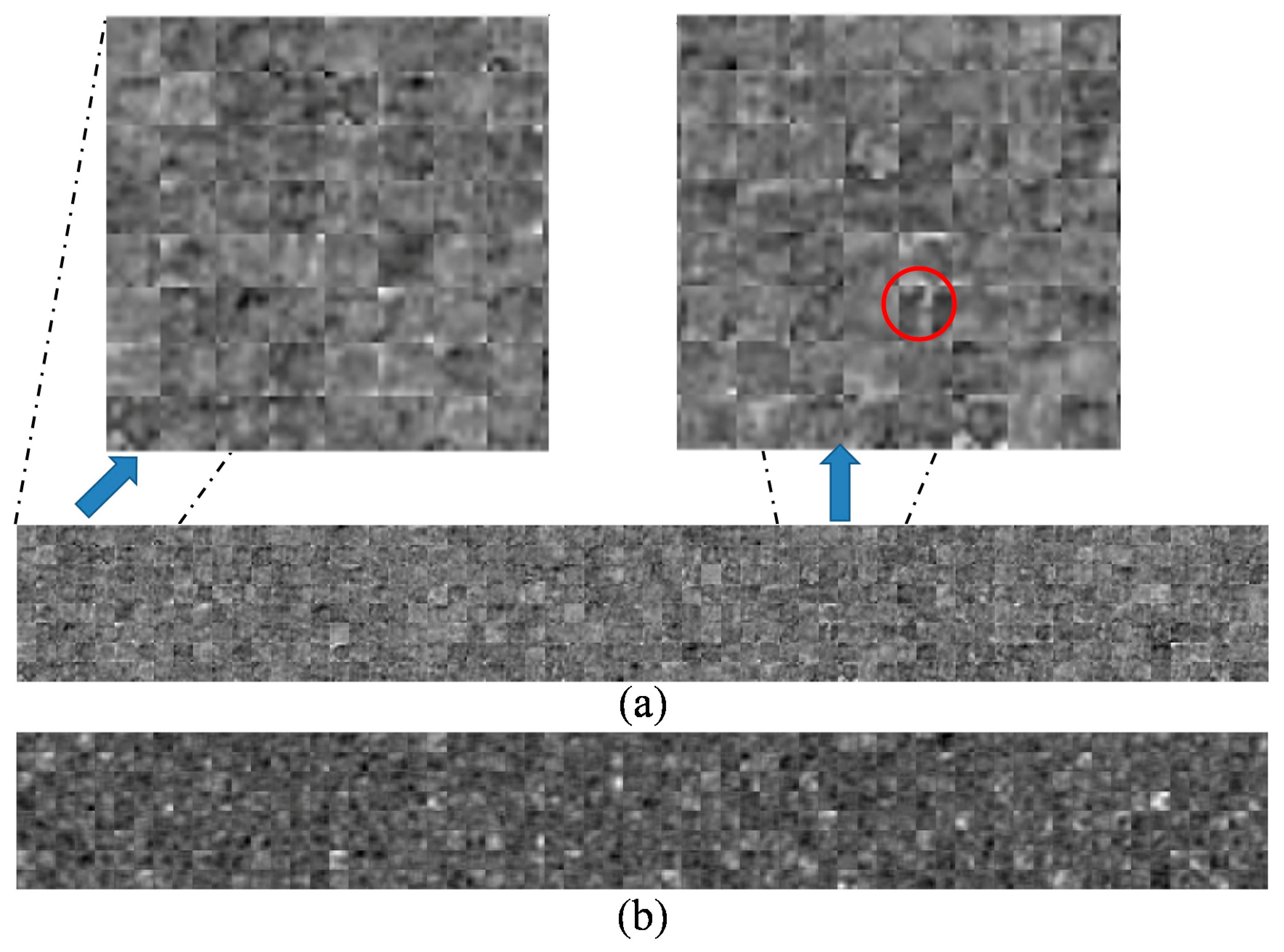
3.3. Visualization of Features

As the feature extractor of the YOLO_v2, the deep CNN network was a key component. In this paper, the features extracted by ‘resnet18’ were visualized to explain the influence of the feature extraction process on the detection results. The feature images of L1~L8 (Figure 5) were displayed respectively. Figure 6 is the feature images of L1 and L2, and 64 feature images were obtained for each layer. Some feature images showed the outline of the crack. But there was interference by other non-target objects (some grass and background).

Figure 7 is the feature images of L3 and L4, and 128 feature images were obtained for each layer. Compared with L1 and L2, the resolution of the feature images was reduced due to the convolution process. Some extra interference was filtered out. The ideal feature (crack shape, marked by a red circle) of the crack was extracted from some feature images. Therefore, using L3 and L4 as a feature extraction layer, the detection effect (Table 4) was better than L1 and L2.

Figure 8 is the feature images of L5 and L6, and 256 feature images were obtained for each layer. The resolution continued to decrease and the features were still visible, as shown in the marked location in Figure 8. Using L5 and L6 as feature extraction layers, the detection performance (Table 4) remained at a high level.

Figure 9 is the feature images of L7 and L8, and 512 feature images were obtained for each layer. At this point, the resolution continued to decrease. At L7, the crack features were still visible, but at L8, the image became extremely fuzzy and the visual features disappeared. This was also confirmed in Table 4 (detection results).

In general, a deeper network layer (deeper layer to get lower resolution feature image) could help to filter out some non-target objects (grass and background). However, it did not mean that the lower the resolution, the better the detection results. If the resolution was too low, it was easy to ignore the features of the object (crack), which can be confirmed in Table 4. Therefore, the selection of the feature extraction layer was worth further studying, which determined the feature information obtained by the YOLO_v2 detection layer. Figure 10 shows some results of crack feature extraction (‘resnet18’ with ‘L6’ feature extraction layer).

4. Conclusions

In this paper, we have compared the detection performance of 11 well-known CNN models as the YOLO_v2 feature extractors and identified an excellent feature extractor based on the precision and computational cost. Then, the parametric studies were carried out: (1) Influence of the training epochs on detection results. (2) The influence of different feature extraction layers on the detection results was compared. (3) The size of the testing images also affects the detection results. The associated parameters indeed have an impact on the detection results. Finally, the working mechanism of the feature extractor was explained by visualizing the features obtained by the feature extractor.

Based on the above research results, this paper draws the following conclusions:

• The comparison of 11 well-known network models indicated that the ‘resnet18’ has a high precision (AP = 0.89) and fast computing speed.
• Influence of relevant parameters on detection results:

  (a)

  Once the detection precision is stable, there is no need to increase the epoch number, which will increase the computing cost.

  (b)

  An appropriate selection of the feature extraction layer can help to improve the detection results. Too shallow or too deep layers can also lead to unsatisfactory detection results.

  (c)

  The detection precision increases with the resolution of the images used; but once it reaches the optimal value, it is meaningless to further increase the image resolution, as it means more detection time.

• In the process of feature visualization, the feature extractor can extract effective crack features and confirms the conclusion of 2 (b).

References

1. Koch, C.; Georgieva, K.; Kasireddy, V.; Akinci, B.; Fieguth, P. A review on computer vision based defect detection and condition assessment of concrete and asphalt civil infrastructure. Adv. Eng. Inform. 2015, 29, 196–210. [Google Scholar] [CrossRef] [Green Version]
2. Prakash, G.; Narasimhan, S.; Al-Hammoud, R. A two-phase model to predict the remaining useful life of corroded reinforced concrete beams. J. Civil Struct. Health Monit. 2019, 9, 183–199. [Google Scholar] [CrossRef]
3. Xu, J.; Gui, C.; Han, Q. Recognition of rust grade and rust ratio of steel structures based on ensembled convolutional neural network. Comput. Aided Civil Infrastruct. Eng. 2020, 35, 1160–1174. [Google Scholar] [CrossRef]
4. Cha, Y.J.; Choi, W.; Suh, G.; Mahmoudkhani, S.; Buyukozturk, O. Autonomous Structural Visual Inspection Using Region-Based Deep Learning for Detecting Multiple Damage Types. Comput. Aided Civil Infrastruct. Eng. 2018, 33, 731–747. [Google Scholar] [CrossRef]
5. Li, G.; Ren, X.; Qiao, W.; Ma, B.; Li, Y. Automatic bridge crack identification from concrete surface using ResNeXt with postprocessing. Struct. Control Health Monit. 2020, 27, e2620. [Google Scholar] [CrossRef]
6. Zhang, C.; Chang, C.C.; Jamshidi, M. Concrete bridge surface damage detection using a single-stage detector. Comput. Aided Civil Infrastruct. Eng. 2019, 35, 389–409. [Google Scholar] [CrossRef]
7. Shi, Y.; Cui, L.; Qi, Z.; Meng, F.; Chen, Z. Automatic Road Crack Detection Using Random Structured Forests. IEEE Trans. Intell. Transp. Syst. 2016, 17, 3434–3445. [Google Scholar] [CrossRef]
8. Jain, A.K.; Mao, J.; Mohiuddin, K.M. Artificial Neural Networks: A Tutorial. Computer 2015, 29, 31–44. [Google Scholar] [CrossRef] [Green Version]
9. Wang, L.; Zhuang, L.; Zhang, Z. Automatic Detection of Rail Surface Cracks with a Superpixel-Based Data-Driven Framework. J. Comput. Civil Eng. 2019, 33, 04018053. [Google Scholar] [CrossRef]
10. Hoang, N.D. An Artificial Intelligence Method for Asphalt Pavement Pothole Detection Using Least Squares Support Vector Machine and Neural Network with Steerable Filter-Based Feature Extraction. Adv. Civil Eng. 2018, 4, 1–12. [Google Scholar] [CrossRef] [Green Version]
11. Yao, X. Evolutionary Artificial Neural Networks. Int. J. Neural Syst. 1993, 4, 203–222. [Google Scholar] [CrossRef]
12. Lin, Y.Z.; Nie, Z.H.; Ma, H.W. Structural Damage Detection with Automatic Feature extraction through Deep Learning. Comput. Aided Civil Infrastruct. Eng. 2017, 32, 1–22. [Google Scholar] [CrossRef]
13. Zhong, K.; Teng, S.; Liu, G.; Chen, G.; Cui, F. Structural Damage Features Extracted by Convolutional Neural Networks from Mode Shapes. Appl. Sci. 2020, 10, 4247. [Google Scholar] [CrossRef]
14. Lecun, Y.; Bengio, Y.; Hinton, G. Deep learning. Nature 2015, 521, 436. [Google Scholar] [CrossRef] [PubMed]
15. Tang, Z.; Chen, Z.; Bao, Y.; Li, H. Convolutional neural network-based data anomaly detection method using multiple information for structural health monitoring. Struct. Control Health Monit. 2019, 26, e2296. [Google Scholar] [CrossRef] [Green Version]
16. Cha, Y.; Choi, W.; Büyüköztürk, O. Deep Learning-Based Crack Damage Detection Using Convolutional Neural Networks. Comput. Aided Civil Infrastruct. Eng. 2017, 32, 361–378. [Google Scholar] [CrossRef]
17. Rafiei, M.H.; Adeli, H. A novel machine learning-based algorithm to detect damage in high-rise building structures. Struct. Des. Tall Spec. Build. 2017, 26, e1400. [Google Scholar] [CrossRef]
18. Teng, S.; Chen, G.; Gong, P.; Liu, G.; Cui, F. Structural damage detection using convolutional neural networks combining strain energy and dynamic response. Meccanica 2019, 55, 945–959. [Google Scholar] [CrossRef]
19. Teng, S.; Chen, G.; Liu, G.; Lv, J.; Cui, F. Modal Strain Energy-Based Structural Damage Detection Using Convolutional Neural Networks. Appl. Sci. 2019, 9, 3376. [Google Scholar] [CrossRef] [Green Version]
20. Gao, Y.; Mosalam, K.M. Deep Transfer Learning for Image-Based Structural Damage Recognition. Comput. Aided Civil Infrastruct. Eng. 2018, 33, 748–768. [Google Scholar] [CrossRef]
21. Kumar, S.S.; Abraham, D.M.; Jahanshahi, M.R.; Iseley, T.; Starr, J. Automated defect classification in sewer closed circuit television inspections using deep convolutional neural networks. Autom. Constr. 2018, 91, 273–283. [Google Scholar] [CrossRef]
22. Krizhevsky, A.; Sutskever, I.; Hinton, G.E. ImageNet Classification with Deep Convolutional Neural Networks. In Proceedings of the International Conference on Neural Information Processing Systems, Lake Tahoe, NV, USA, 3–6 December 2012; pp. 1097–1105. [Google Scholar]
23. Zhang, A.; Wang, K.C.P.; Li, B.; Yang, E.; Dai, X.; Peng, Y.; Fei, Y.; Liu, Y.; Li, J.Q.; Chen, C. Automated Pixel-Level Pavement Crack Detection on 3D Asphalt Surfaces Using a Deep-Learning Network. Comput. Aided Civil Infrastruct. Eng. 2017, 32, 805–819. [Google Scholar] [CrossRef]
24. Li, B.; Wang, K.C.P.; Zhang, A.; Yang, E.; Wang, G. Automatic classification of pavement crack using deep convolutional neural network. Int. J. Pavement Eng. 2020, 21, 457–463. [Google Scholar] [CrossRef]
25. Hiroya, M.; Yoshihide, S.; Toshikazu, S.; Takehiro, K.; Hiroshi, O. Road Damage Detection and Classification Using Deep Neural Networks with Smartphone Images. Comput. Aided Civil Infrastruct. Eng. 2018, 33, 1127–1141. [Google Scholar]
26. Kaur, T.; Gandhi, T.K. Automated Brain Image Classification Based on VGG-16 and Transfer Learning. In Proceedings of the 2019 International Conference on Information Technology (ICIT), Bhubaneswar, India, 19–21 December 2019. [Google Scholar]
27. Liang, Y.; Bing, L.; Wei, L.; Liu, Z.; Xiao, J. Deep Concrete Inspection Using Unmanned Aerial Vehicle Towards CSSC Database. In Proceedings of the 2017 IEEE/RSJ International Conference on Intelligent Robots and Systems, Vancouver, BC, Canada, 24–28 September 2017; pp. 24–28. [Google Scholar]
28. Yeum, C.M.; Dyke, S.J.; Ramirez, J. Visual data classification in post-event building reconnaissance. Eng. Struct. 2018, 155, 16–24. [Google Scholar] [CrossRef]
29. Ren, S.; He, K.; Girshick, R.; Sun, J. Faster R-CNN: Towards Real-Time Object Detection with Region Proposal Networks. IEEE Trans. Pattern Anal. Mach. Intell. 2017, 39, 1137–1149. [Google Scholar] [CrossRef] [Green Version]
30. Xu, Y.; Wei, S.; Bao, Y.; Li, H. Automatic seismic damage identification of reinforced concrete columns from images by a region-based deep convolutional neural network. Struct. Control Health Monit. 2019, 26, e2313. [Google Scholar] [CrossRef]
31. Liang, X. Image-based post-disaster inspection of reinforced concrete bridge systems using deep learning with Bayesian optimization. Comput. Aided Civil Infrastruct. Eng. 2018, 3, 112–119. [Google Scholar] [CrossRef]
32. Tran, V.P.; Tran, T.S.; Lee, H.J.; Kim, K.D.; Baek, J.; Nguyen, T.T. One stage detector (RetinaNet)-based crack detection for asphalt pavements considering pavement distresses and surface objects. J. Civil Struct. Health Monit. 2020. [Google Scholar] [CrossRef]
33. Lattanzi, D.; Miller, G. Review of Robotic Infrastructure Inspection Systems. J. Infrastruct. Syst. 2017, 23, 04017004. [Google Scholar] [CrossRef]
34. Yin, X.; Chen, Y.; Bouferguene, A.; Zaman, H.; Kurach, L. A deep learning-based framework for an automated defect detection system for sewer pipes. Autom. Constr. 2019, 109, 102967. [Google Scholar] [CrossRef]
35. Liu, J.; Yang, X.; Lau, S.; Wang, X.; Luo, S.; Lee, V.C.-S.; Ding, L. Automated pavement crack detection and segmentation based on two-step convolutional neural network. Comput. Aided Civil Infrastruct. Eng. 2020, 35, 1291–1305. [Google Scholar] [CrossRef]
36. Li, R.; Yuan, Y.; Zhang, W.; Yuan, Y. Unified Vision-Based Methodology for Simultaneous Concrete Defect Detection and Geolocalization. Comput. Aided Civil Infrastruct. Eng. 2018, 33, 527–544. [Google Scholar] [CrossRef]
37. Redmon, J.; Divvala, S.; Girshick, R.; Farhadi, A. You Only Look Once: Unified, Real-Time Object Detection. In Proceedings of the IEEE Conference on Computer Vision and Pattern Recognition, Las Vegas, NV, USA, 27–30 June 2016; pp. 779–788. [Google Scholar]
38. Russakovsky, O.; Deng, J.; Su, H.; Krause, J.; Satheesh, S.; Ma, S.; Huang, Z.; Karpathy, A.; Khosla, A.; Bernstein, M. ImageNet Large Scale Visual Recognition Challenge. Int. J. Comput. Vis. 2015, 115, 211–252. [Google Scholar] [CrossRef] [Green Version]
39. Available online: http://www.mathworks.com/ (accessed on 14 December 2020).
40. Mandt, S.; Hoffman, M.D.; Blei, D.M. Stochastic Gradient Descent as Approximate Bayesian Inference. J. Mach. Learn. Res. 2017, 18, 1–35. [Google Scholar]
Figure 1. The YOLO_v2 architecture.
Applsci 11 00813 g001
Figure 2. Locate the anchor box using the detection layer.
Applsci 11 00813 g002
Figure 3. Labeled images by the ‘Image labeler’ toolbox.
Applsci 11 00813 g003
Figure 4. The AP value and computational cost of different epochs. (a) AP value; (b) computational cost.
Applsci 11 00813 g004
Figure 5. The architecture of the ‘resnet18’.
Applsci 11 00813 g005
Figure 6. Feature images of L1 and L2. (a) Raw image; (b) Feature images of L1 (64 images); (c) Feature images of L2 (64 images).
Applsci 11 00813 g006
Figure 7. Feature images of L3 and L4. (a) Feature images of L3 (128 images); (b) Feature images of L4 (128 images).
Applsci 11 00813 g007
Figure 8. Feature images of L5 and L6. (a) Feature images of L5 (256 images); (b) Feature images of L6 (256 images).
Applsci 11 00813 g008
Figure 9. Feature images of L7 and L8. (a) Feature images of L7 (512 images); (b) Feature images of L8 (512 images).
Applsci 11 00813 g009
Figure 10. Results of crack feature extraction.
Applsci 11 00813 g010