Modified Viterbi Algorithm with Feedback Using a Two-Dimensional 3-Way Generalized Partial Response Target for Bit-Patterned Media Recording Systems

Abstract

The ever-increasing demand for data in recent times has led to the emergence of big data and cloud data. The growth in these fields has necessitated that data be centrally stored in data centers. To meet the need for large-scale storage systems at data centers, innovative technology such as bit-pattern media recording (BPMR) has been developed. With BPMR technology, we are able to achieve significant improvements in high areal density (AD) of magnetic data storage systems. However, two-dimensional (2D) interference is a common issue faced with high AD. Intersymbol interference and intertrack interference occur when the distance between the islands is decreased in the down-track and cross-track, respectively. 2D interference adversely affects the performance of BPMR. In this paper, we propose an improved modified Viterbi algorithm (MVA) exploiting a feedback and a new 2D three-way form of a generalized partial response (GPR) target. The proposed MVA with feedback is superior to the previous MVA by eliminating intertrack interference (ITI) more effectively. With the three-way GPR target, the proposed algorithm achieves more stable performance compared to the previous detection algorithms for the track misregistration effect.

1. Introduction

With the proliferation of electronic devices, more data are constantly being generated and consumed on a daily basis. Initially, massive amounts of data were mainly produced by industrial applications. However, the advent of handhelds and social networks resulted in more data being generated at a faster rate. Additionally, the Internet of Things, which is a system of interrelated devices, is able to create and transmit data. The scale of data owing to the factors mentioned above is commonly described as big data. The data are usually centrally stored in data centers. Data centers are often required to increase their storage capacity owing to the growth in big data and cloud data services. Cloud data services have become very popular owing to their many advantages such as data synchronization across all devices and improved data security. The transition to centralized storage has also been accelerated by the implementation of 5G technology, which offers significantly higher internet speeds. To build data centers with high storage capacity, two technologies exist, namely solid state and magnetic storage. The choice is a trade-off between access speed and price per bit. The price per bit for magnetic storage is much lower than that for solid-state storage [1]. The areal density (AD) for magnetic storage is limited to approximately 1 terabit per square inch (Tb/in²) (0.155 Tb/cm²) owing to the superparamagnetic phenomenon [2]. To combat this problem, several new technologies have been proposed, such as heat-assisted magnetic recording [3], microwave-assisted magnetic recording [4], two-dimensional (2D) magnetic recording [5], and bit-patterned media recording (BPMR) [6].

BPMR is an extremely promising technology to overcome the AD limitations seen in existing magnetic storage. For BPMR-based systems, data bits are stored on magnetic islands. To increase the AD, the distance between the magnetic islands has to be reduced. This increases the intersymbol interference (ISI) and intertrack interference (ITI) in the down-track and cross-track direction, respectively. Owing to the increase in 2D interference, such as ISI and ITI, the BPMR channel performance in terms of bit error rate (BER) is negatively affected.

Error correction codes and modulation code are two common methods to minimize 2D interference in signal processing. Jeong and Lee [7] proposed the use of modulation code and multilayer perceptron decoding for BPMR to reduce and correct errors due to ITI, respectively. Error-correcting 5/6 modulation code was introduced [8] by Nguyen and Lee to reduce 2D interference and correct errors. Buajong proposed a combination of rate-3/4 modulation code and ITI subtraction in [9] to reduce ITI. In addition, we can use an equalizer and detector with a generalized partial response (GPR) target to minimize 2D interference. Additionally, Kim proposed a 2D soft-output Viterbi algorithm (2D SOVA) [10] to reduce the effects of 2D interference. The 2D SOVA method was further developed as an iterative 2D SOVA for bit-patterned media [11]. In addition, the modified Viterbi algorithm (MVA) proposed by Nabavi, Kumar, and Zhu in [12] is widely used [13,14,15,16]. However, the MVA [12] was only used as part of the detector in their study. Therefore, in this paper, we propose a three-way GPR utilizing a three-way MVA [12] with feedback. This is a huge improvement over the original MVA [12] standalone implementation. Besides, there are detection schemes based on the Bahl-Cocke-Jelinek-Raviv (BCJR) algorithm [17,18]. In [17], an iterative row-column soft decision feedback algorithm (IRCSDFA) is presented. Then, in [18], the IRCSDFA reduced the complexity by applying Gaussian approximation (IRCSDFA-GA). Although IRCSDFA-GA has low complexity compared to IRCSDFA, the main detection is still the BCJR algorithm, which is much more complex than the MVA.

The rest of the paper is divided as follows. Section 2 discusses the N-way GPR target and N-way detection. Section 3 explains the proposed model and details of our algorithm. The simulation results and conclusions are discussed in Section 4 and Section 5, respectively.

2. N-Way GPR Target and N-Way Detection

In this study, we propose a method utilizing an N-way GPR target and N-way detection where N is the number of neighboring symbols affecting the current symbol.

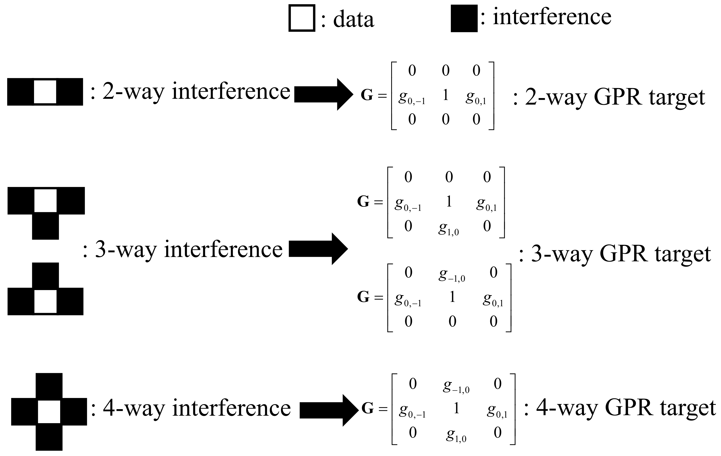
2.1. N-Way GPR Target

To understand the N-way GPR target works, we will first explain N-way interference. Consider a channel with matrix C as follows:

$$C=\left[\begin{array}{ccc}0& c_{-1,0}& 0\\ c_{0,-1}& c_{0,0}& c_{0,1}\\ 0& c_{1,0}& 0\end{array}\right]$$

(1)

If we send a serial one-dimensional (1D) signal through the channel C, the interference affecting both sides of the current symbol, also known as a two-way interference, is represented by the coefficients c_0,−1 and c_0,1. If we send a 2D signal through the channel, the interference affecting the signal will instead be on four sides of the current symbol represented by the coefficients c_0,−1, c_0,1, c_−1,0, and c_1,0. This is referred to as four-way interference. For three-way interference, we look at the data edge of the 2D signal (as shown in Figure 1). At the data edges, the interference coefficient is equal to 0 at one of the four-way interference paths, because there is no signal at that interference coefficient. For example, for the data at the left edge, the interference coefficient c_0,−1 becomes zero, and at the top edge, coefficient c_−1,0 is equal to zero.

To estimate the coefficient of the N-way interference, we utilize its associated N-way GPR target. In Figure 2, we summarize the N-way GPR target.

The first example illustrates the interference from the left and right side of the current data. In this case, it is referred to as two-way interference and a two-way GPR target. In the second example, the interference is from the left, right, and upper (or lower) sides of the data. This is referred to as three-way interference and a three-way GPR target. In the final one, we have interference coming from the left, right, upper, and lower sides of the data. This is referred to as four-way interference and a four-way GPR target.

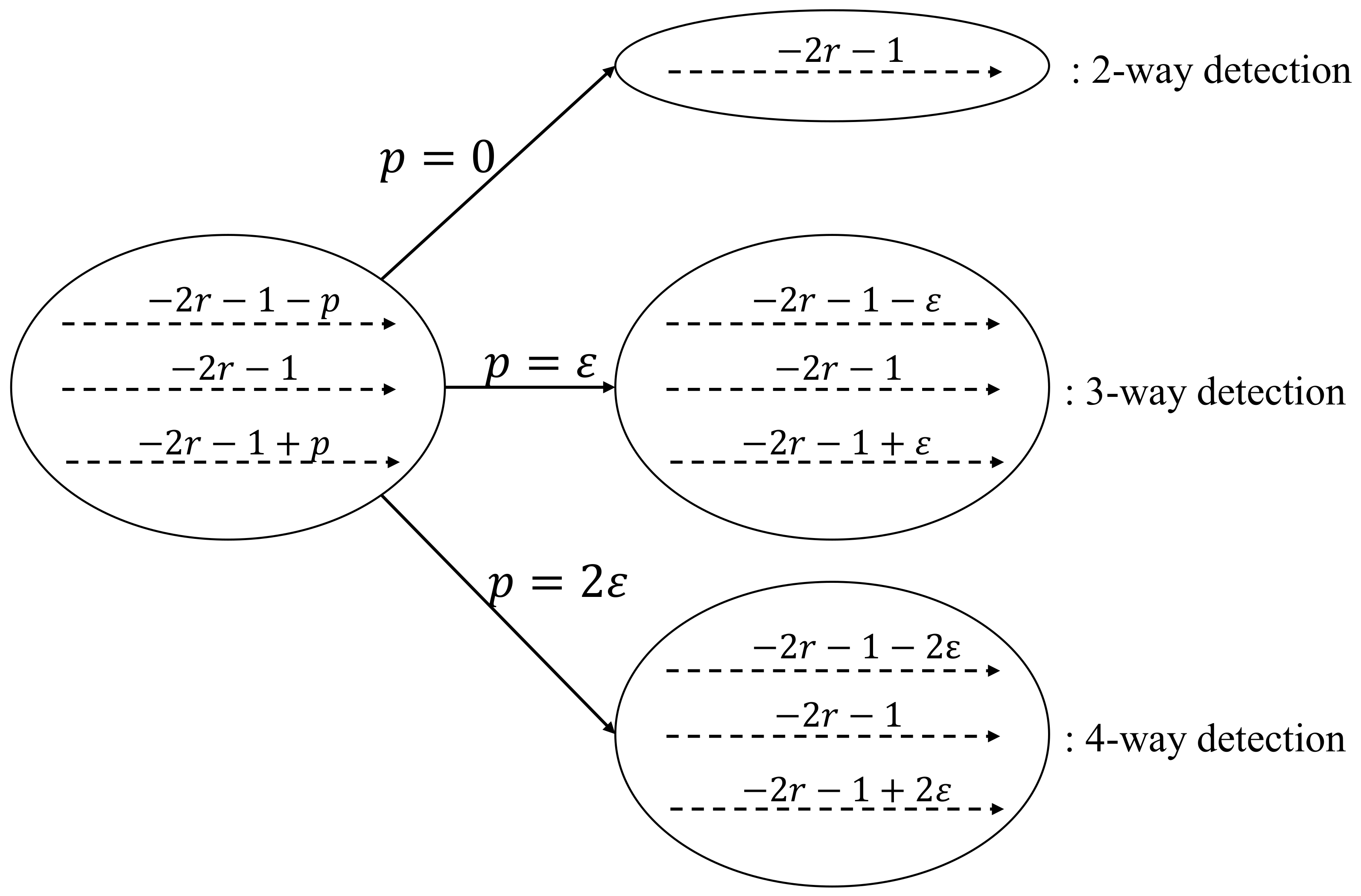
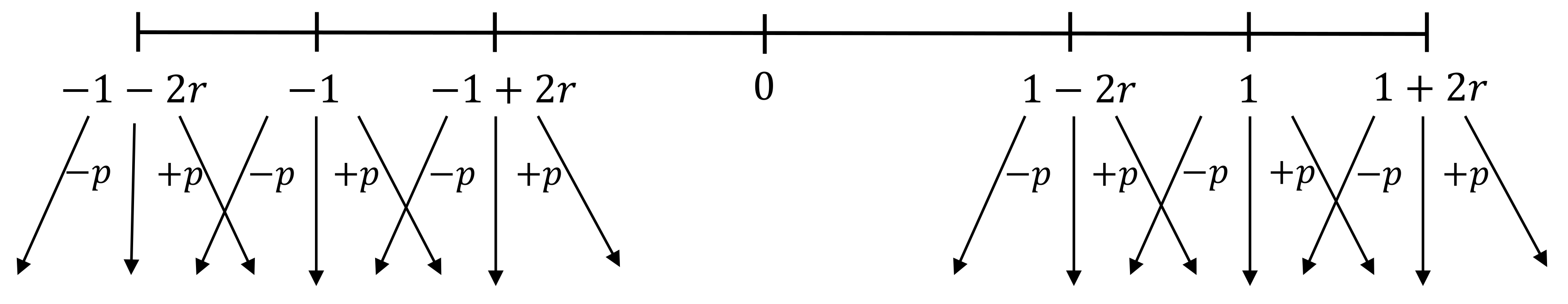
2.2. N-Way Detection

When estimating a GPR target, the output signal will be similar to the original signal passing through the target. Therefore, the target structure has an effect on the value of the output signal. As the channels are usually symmetrical, we can assume that the 2D target will be in the following form irrespective of ITI.

$$G=\left[\begin{array}{ccc}0& 0& 0\\ r& 1& r\\ 0& 0& 0\end{array}\right]$$

(2)

The output signal for this target, which includes [−2r − 1, −1, 2r − 1, −2r + 1, 1, 2r + 1], is listed in the form of a trellis diagram as shown in Figure 3:

The detection scheme described above is known as the conventional Viterbi algorithm (VA). To implement the MVA [12], we would need to add and subtract a small coefficient p to the output value in each branch. The trellis diagram of the MVA is shown in Figure 4.

In the MVA, the upper and lower channel interference coefficients are denoted by $\epsilon$, corresponding to four-way interference. Therefore, the detection for four-way interference is equivalent to four-way detection. In addition, as $\epsilon$ interference originates from above and below the signal, p = $2\epsilon$. For three-way interference, the trellis diagram for the MVA was used, and the corresponding detection was a three-way detection with p = $\epsilon$. This is due to the $\epsilon$ interference originating only from above or below the signal. Finally, in the case of two-way interference, the corresponding detection is a two-way detection, where p = 0. The trellis diagram is the same as the conventional Viterbi algorithm (VA). Figure 5 illustrates the branch values for each N-way detection.

In [12], the MVA is a combination of the two-way GPR target and four-way detection to minimize ITI. As the two-way GPR target was used, an appropriate ε had to be determined and kept constant for the algorithm. In our proposal, we used a three-way GPR target to help estimate ε. In other words, ε and the GPR target were estimated simultaneously.

In the proposed model, we use a GPR target represented in matrix form G_u and G_l such as Equation (3). The matrix consists of the three-way interference information relating to ITI interference.

$$G_u=\left[\begin{array}{ccc}0& g_{-1,0}& 0\\ g_{0,-1}& 1& g_{0,1}\\ 0& 0& 0\end{array}\right]\hspace{1em}\mathrm{or}\hspace{1em}{G}_l=\left[\begin{array}{ccc}0& 0& 0\\ g_{0,-1}& 1& g_{0,1}\\ 0& g_{1,0}& 0\end{array}\right]$$

(3)

However, ITI may be added to the signal when applying the three-way interference. Therefore, to eliminate ITI, we implemented a feedback path at the detector. Finally, we use a three-way MVA to match the three-way GPR target. The results show that our proposed model achieves higher BER performance compared to the MVA [12] by itself.

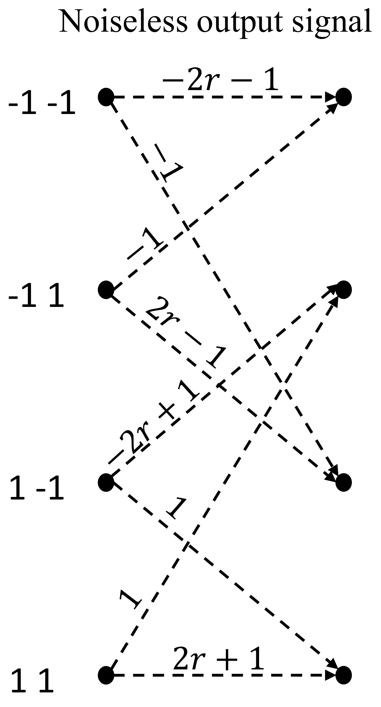
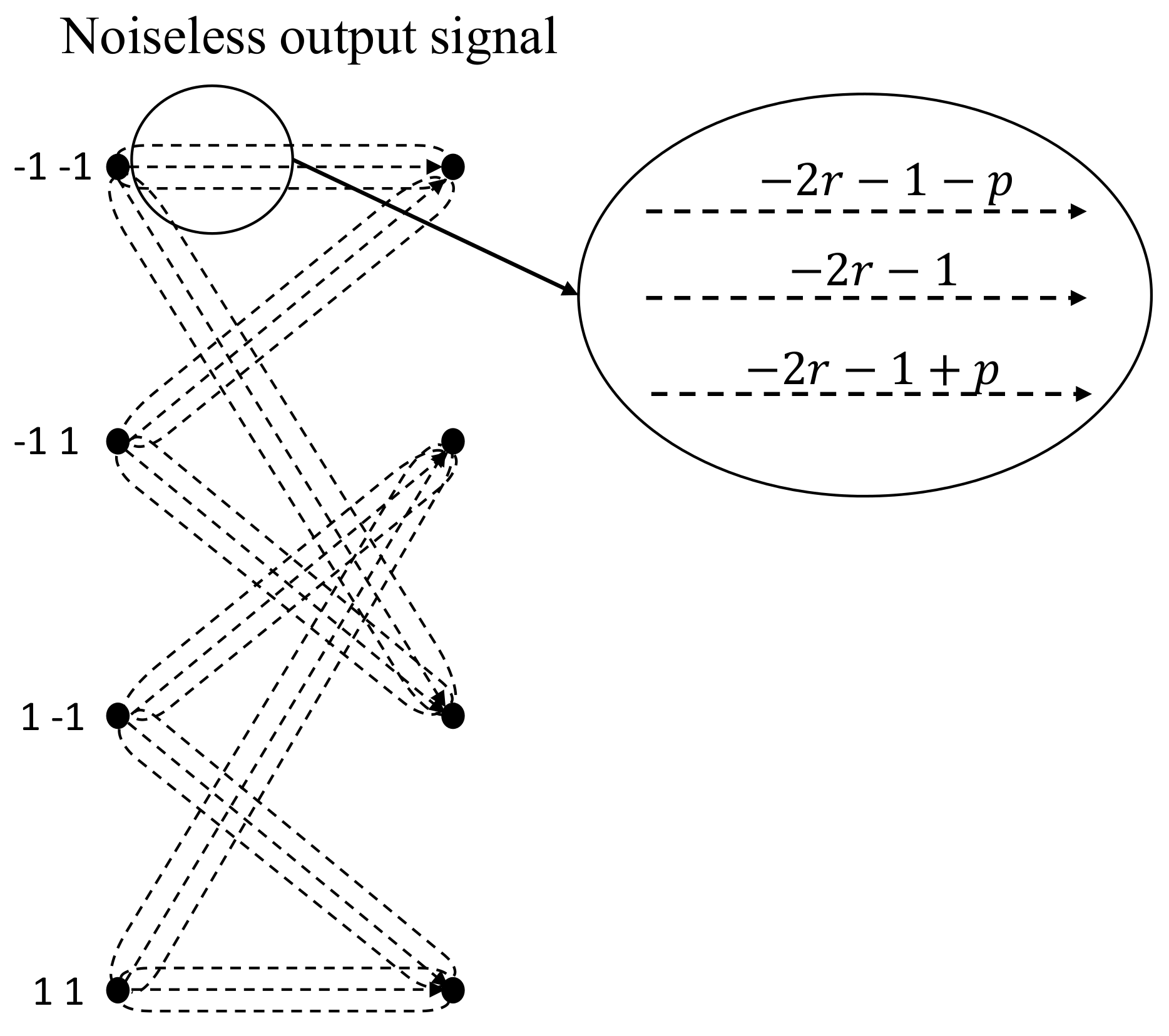
2.3. Alias Phenomenon of the Output Value

Figure 6 illustrates that the output values of the trellis diagram can be aliased if p is large. In conventional trellis, the output value of each branch is distinct because r is a small value compared to 1. For the modified trellis, p is added or subtracted from the output values. Therefore, the output branches can overlap because r is on a similar scale to p. For example, the branch from (−1 −1) to (−1 −1) in conventional trellis will have a value of −2r − 1. However, in modified trellis, there are three possible branch values, namely −2r–1 − p, −2r − 1, and −2r–1 + p. If the p value is too large, the value of −2r–1 + p will be greater than the value of −1 − p or potentially greater than −1. Therefore, the branch from (−1 −1) to (−1 −1) may be confused with the branch from (−1 −1) to (1 −1). We refer to the overlapping of these values as the alias phenomenon. This phenomenon decreases the BER performance, i.e., a higher alias results in lower performance.

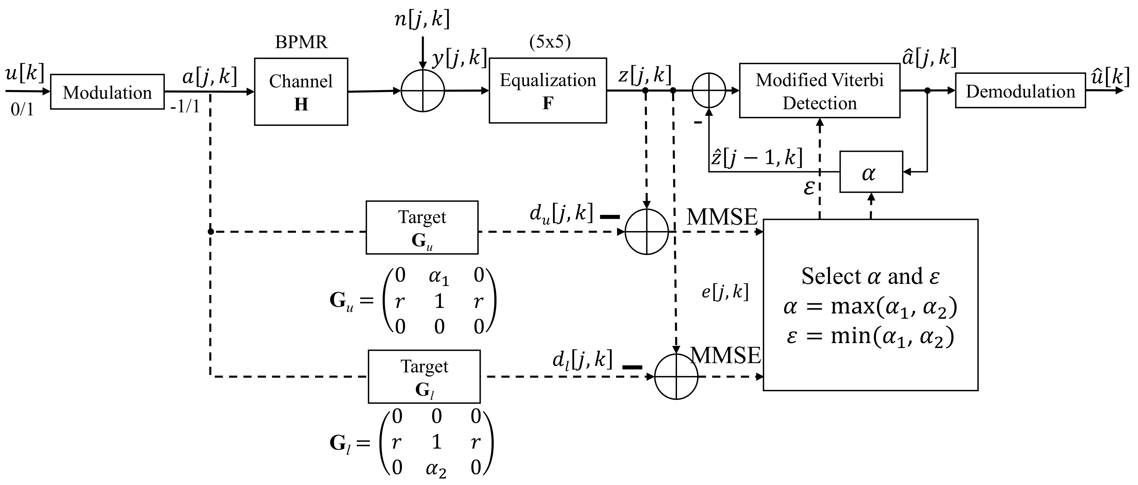
3. Proposed System Model

In this paper, we proposed a 2D three-way GPR target and three-way MVA with feedback. Our model is applied to the BPMR channel. In addition, we use a 2D equalizer instead of a 1D equalizer in the MVA [12]. Our proposed system model is shown in Figure 7.

In the proposed model, the original data u[k] are modulated into a[j,k] and stored on the BPMR system. The BPMR channel, which includes the 2D ISI and electronic and media noise, is presented in Section 3.1. The output of the BPMR channel y[j,k] is balanced by equalization F, which is explained in Section 3.2. The estimation of the equalization F is implemented immediately after the estimation of the target G_u and G_l. After finishing the training process, the parameters $\alpha$ and $\epsilon$ are decided by ${\alpha }_1$ and ${\alpha }_2$ of G_u and G_l, respectively. The equalizer output z[j,k] is detected by the proposed detection algorithm, which is analyzed in Section 3.3. Finally, the output of detector $\widehat{a}\left[j,k\right]\in \left[-1,1\right]$ is demodulated into the original signal $\widehat{u}\left[j,k\right]\in \left[0,1\right]$.

3.1. BPMR Channel

Before putting data through the channel, input data u[k] $\in$ {0,1} are magnetized into 2D data a[j,k] $\in$ {−1,1}. Data a[j,k] are then passed through the BPMR channel. At the receiver, the received data are modeled as additive white Gaussian noise (AWGN). For the simulations, a 2D Gaussian pulse response, representing the 2D island response for the BPMR channel, is expressed as follows [19,20,21]:

$$P\left(x,z\right)=A\exp \left(-\frac{1}{2c^2}\left[{\left(\frac{x+{\Delta }_x}{P{W}_x}\right)}^2+{\left(\frac{z+{\Delta }_z}{P{W}_z}\right)}^2\right]\right),$$

(4)

where x and z are the down- and cross-track directions, respectively; ${\Delta }_x$ and ${\Delta }_z$ are the down- and cross-track bit location fluctuations, respectively; c represents the relationship between the standard deviation of a Gaussian function and PW₅₀, which is the pulse width at half the peak amplitude, and c is 1/2.3548; and PW_x and PW_z are the PW₅₀ components of the down- and cross-track pulses, respectively.

The BPMR 2D channel island pulse response is expressed as follows:

$$h\left[j,k\right]=P\left(j{T}_x,k{T}_z\pm {\Delta }_{off}\right),$$

(5)

where j and k are the discrete indices in the down- and cross-track directions, respectively; T_x and T_z are the bit period and track pitch, respectively; and ${\Delta }_{off}$ is the read-head offset for the cross-track. Track misregistration (TMR) is defined as the head offset size divided by the magnetic-island period and can be expressed as follows:

$$\mathrm{TMR}\left(\%\right)=\frac{{\Delta }_{off}}{T_z}.$$

(6)

Readback signal y[j,k] for BPMR is given by

$$y\left[j,k\right]=a\left[j,k\right]*h\left[j,k\right]+n\left[j,k\right],$$

(7)

where a[j,k], h[j,k], and n[j,k] are the 2D discrete input data, 2D channel response, and electronic noise modeled as AWGN with zero mean and variance ${\sigma }^2$, respectively.

3.2. Equalizer and GPR Target

In Figure 7, the equalizer is combined with the GPR target [22]. Here, the equalizer and GPR target are represented by matrix F and matrix G, respectively.

$$\mathbf{F}=\left[\begin{array}{ccccc}{f}_{-2,-2}& f_{-2,-1}& f_{-2,0}& f_{-2,1}& f_{-2,2}\\ f_{-1,-2}& f_{-1,-1}& f_{-1,0}& f_{-1,1}& f_{-1,2}\\ f_{0,-2}& f_{0,-1}& f_{0,0}& f_{0,1}& f_{0,2}\\ f_{1,-2}& f_{1,-1}& f_{1,0}& f_{1,1}& f_{1,2}\\ f_{2,-2}& f_{2,-1}& f_{2,0}& f_{2,1}& f_{2,2}\end{array}\right]$$

(8)

$$\mathbf{G}=\left[\begin{array}{ccc}{g}_{-1,-1}& g_{-1,0}& g_{-1,1}\\ g_{0,-1}& g_{0,0}& g_{0,1}\\ g_{1,-1}& g_{1,0}& g_{1,1}\end{array}\right]$$

(9)

The output of equalizer z[j,k] is the 2D convolution of equalizer F and channel output y[j,k]. The output of target d[j,k] is also the 2D convolution of target G and input data a[j,k]. These outputs can be expressed as follows:

$$z\left[j,k\right]={\mathbf{f}}^T\mathbf{y}$$

(10)

$$d\left[j,k\right]={\mathbf{g}}^T\mathbf{a}$$

(11)

where

$$\mathbf{f}={\left[\begin{array}{ccccccc}{f}_{-2,-2}& f_{-2,-1}& \dots & 0& \dots & f_{2,1}& f_{2,2}\end{array}\right]}^T$$

(12)

$$\mathbf{g}={\left[\begin{array}{ccccccc}{g}_{-1,-1}& g_{-1,0}& \dots & 0& \dots & g_{1,0}& g_{1,1}\end{array}\right]}^T$$

(13)

$$\mathbf{y}={\left[\begin{array}{ccccccc}{y}_{j+2,k+2}& y_{j+2,k+1}& \dots & 0& \dots & y_{j-2,k-1}& y_{j-2,k-2}\end{array}\right]}^T$$

(14)

$$\mathbf{a}={\left[\begin{array}{ccccccc}{a}_{j+1,k+1}& a_{j+1,k}& \dots & 0& \dots & a_{j-1,k}& a_{j-1,k-1}\end{array}\right]}^T$$

(15)

We define the error signal e[j,k] between the equalizer and GPR target as follows:

$$e\left[j,k\right]=z\left[j,k\right]-d\left[j,k\right]$$

(16)

Using expressions (10), (11), and (16), we can calculate the error as follows:

$$e\left[j,k\right]={\mathbf{f}}^T\mathbf{y}-{\mathbf{g}}^T\mathbf{a}$$

(17)

Then, the mean square error (MSE) can be expressed as follows:

$$\begin{array}{ll}E\left\{{\left(e\left[j,k\right]\right)}^2\right\}& =E\left\{\left({\mathbf{f}}^T\mathbf{y}-{\mathbf{g}}^T\mathbf{a}\right){\left({\mathbf{f}}^T\mathbf{y}-{\mathbf{g}}^T\mathbf{a}\right)}^T\right\}\\ & ={\mathbf{f}}^T\mathbf{Rf}-2{\mathbf{f}}^T\mathbf{Tg}+{\mathbf{g}}^T\mathbf{Ag}\end{array}$$

(18)

where R is the auto-correlation matrix of the channel output data, T is the cross-correlation between the input data and the channel output data, and A is the auto-correlation of the input data. Specifically, R = E{yy^T}, T = E{ya^T}, and A = E{aa^T}, where E denotes the expectation, and T is the transpose operator.

To invalidate the trivial condition of f = g = 0 to minimize the MSE in (18), a different constraint should be imposed on g depending on the N-way GPR targets. First, we will set the constraint for the two-way GPR target. The matrix form G for the two-way GPR target is given below.

$$\mathbf{G}=\left[\begin{array}{ccc}0& 0& 0\\ g_{0,-1}& 1& g_{0,1}\\ 0& 0& 0\end{array}\right]$$

(19)

$$g={\left[\begin{array}{ccccccccc}0& 0& 0& g_{0,-1}& 1& g_{0,1}& 0& 0& 0\end{array}\right]}^T$$

(20)

The constraint can be expressed as follows:

$${\mathbf{E}}^T\mathbf{g}=\mathbf{c}$$

(21)

where

$$\mathbf{c}={\left[\begin{array}{ccccccc}0& 0& 0& 1& 0& 0& 0\end{array}\right]}^T$$

(22)

and

$${\mathbf{E}}^T=\left[\begin{array}{ccccccccc}1& 0& 0& 0& 0& 0& 0& 0& 0\\ 0& 1& 0& 0& 0& 0& 0& 0& 0\\ 0& 0& 1& 0& 0& 0& 0& 0& 0\\ 0& 0& 0& 0& 1& 0& 0& 0& 0\\ 0& 0& 0& 0& 0& 0& 1& 0& 0\\ 0& 0& 0& 0& 0& 0& 0& 1& 0\\ 0& 0& 0& 0& 0& 0& 0& 0& 1\end{array}\right]$$

(23)

For the three-way GPR target on the upper ITI, the matrix form G_u is as follows:

$${\mathbf{G}}_u=\left[\begin{array}{ccc}0& g_{-1,0}& 0\\ g_{0,-1}& 1& g_{0,1}\\ 0& 0& 0\end{array}\right]$$

(24)

$$g={\left[\begin{array}{ccccccccc}0& g_{-1,0}& 0& g_{0,-1}& 1& g_{0,1}& 0& 0& 0\end{array}\right]}^T$$

(25)

The constraint can be expressed as follows:

$${\mathbf{E}}^T\mathbf{g}=\mathbf{c}$$

(26)

where

$$\mathbf{c}={\left[\begin{array}{cccccc}0& 0& 1& 0& 0& 0\end{array}\right]}^T$$

(27)

and

$${\mathbf{E}}^T=\left[\begin{array}{ccccccccc}1& 0& 0& 0& 0& 0& 0& 0& 0\\ 0& 0& 1& 0& 0& 0& 0& 0& 0\\ 0& 0& 0& 0& 1& 0& 0& 0& 0\\ 0& 0& 0& 0& 0& 0& 1& 0& 0\\ 0& 0& 0& 0& 0& 0& 0& 1& 0\\ 0& 0& 0& 0& 0& 0& 0& 0& 1\end{array}\right]$$

(28)

For the three-way GPR target on the lower ITI, the matrix form G_l is as follows:

$${\mathbf{G}}_l=\left[\begin{array}{ccc}0& 0& 0\\ g_{0,-1}& 1& g_{0,1}\\ 0& g_{1,0}& 0\end{array}\right]$$

(29)

$$g={\left[\begin{array}{ccccccccc}0& 0& 0& g_{0,-1}& 1& g_{0,1}& 0& g_{1,0}& 0\end{array}\right]}^T$$

(30)

The constraint can be expressed as follows:

$${\mathbf{E}}^T\mathbf{g}=\mathbf{c}$$

(31)

where

$$\mathbf{c}={\left[\begin{array}{cccccc}0& 0& 0& 1& 0& 0\end{array}\right]}^T$$

(32)

and

$${\mathbf{E}}^T=\left[\begin{array}{ccccccccc}1& 0& 0& 0& 0& 0& 0& 0& 0\\ 0& 1& 0& 0& 0& 0& 0& 0& 0\\ 0& 0& 1& 0& 0& 0& 0& 0& 0\\ 0& 0& 0& 0& 1& 0& 0& 0& 0\\ 0& 0& 0& 0& 0& 0& 1& 0& 0\\ 0& 0& 0& 0& 0& 0& 0& 0& 1\end{array}\right]$$

(33)

Finally, for the four-way GPR target [20], the matrix form G is as follows:

$$\mathbf{G}=\left[\begin{array}{ccc}0& g_{-1,0}& 0\\ g_{0,-1}& 1& g_{0,1}\\ 0& g_{1,0}& 0\end{array}\right]$$

(34)

$$g={\left[\begin{array}{ccccccccc}0& g_{-1,0}& 0& g_{0,-1}& 1& g_{0,1}& 0& g_{1,0}& 0\end{array}\right]}^T$$

(35)

The constraint can be expressed as follows:

$${\mathbf{E}}^T\mathbf{g}=\mathbf{c}$$

(36)

where

$$\mathbf{c}={\left[\begin{array}{ccccc}0& 0& 1& 0& 0\end{array}\right]}^T$$

(37)

and

$${\mathbf{E}}^T=\left[\begin{array}{ccccccccc}1& 0& 0& 0& 0& 0& 0& 0& 0\\ 0& 0& 1& 0& 0& 0& 0& 0& 0\\ 0& 0& 0& 0& 1& 0& 0& 0& 0\\ 0& 0& 0& 0& 0& 0& 1& 0& 0\\ 0& 0& 0& 0& 0& 0& 0& 0& 1\end{array}\right]$$

(38)

With these constraints, we can derive the following Lagrange function:

$$J={\mathbf{f}}^T\mathbf{Rf}-2{\mathbf{f}}^T\mathbf{Tg}+{\mathbf{g}}^T\mathbf{Ag}-2{\mathsf{\lambda }}^T\left({\mathbf{E}}^T\mathbf{g}-\mathbf{c}\right)$$

(39)

where $\lambda$ is a vector containing the Lagrange multipliers. By setting the gradients of J with respect to f, g, and $\lambda$ to zero vectors, we obtain the optimized target and equalizer coefficient vectors as follows:

$$\lambda ={\left({\mathbf{E}}^T{\left(\mathbf{A}-{\mathbf{T}}^T{\mathbf{R}}^{-1}\mathbf{T}\right)}^{-1}\mathbf{E}\right)}^{-1}\mathbf{c}$$

(40)

$$\mathbf{g}={\left(\mathbf{A}-{\mathbf{T}}^T{\mathbf{R}}^{-1}\mathbf{T}\right)}^{-1}\mathbf{E}\mathsf{\lambda }$$

(41)

$$\mathbf{f}={\mathbf{R}}^{-1}\mathbf{Tg}$$

(42)

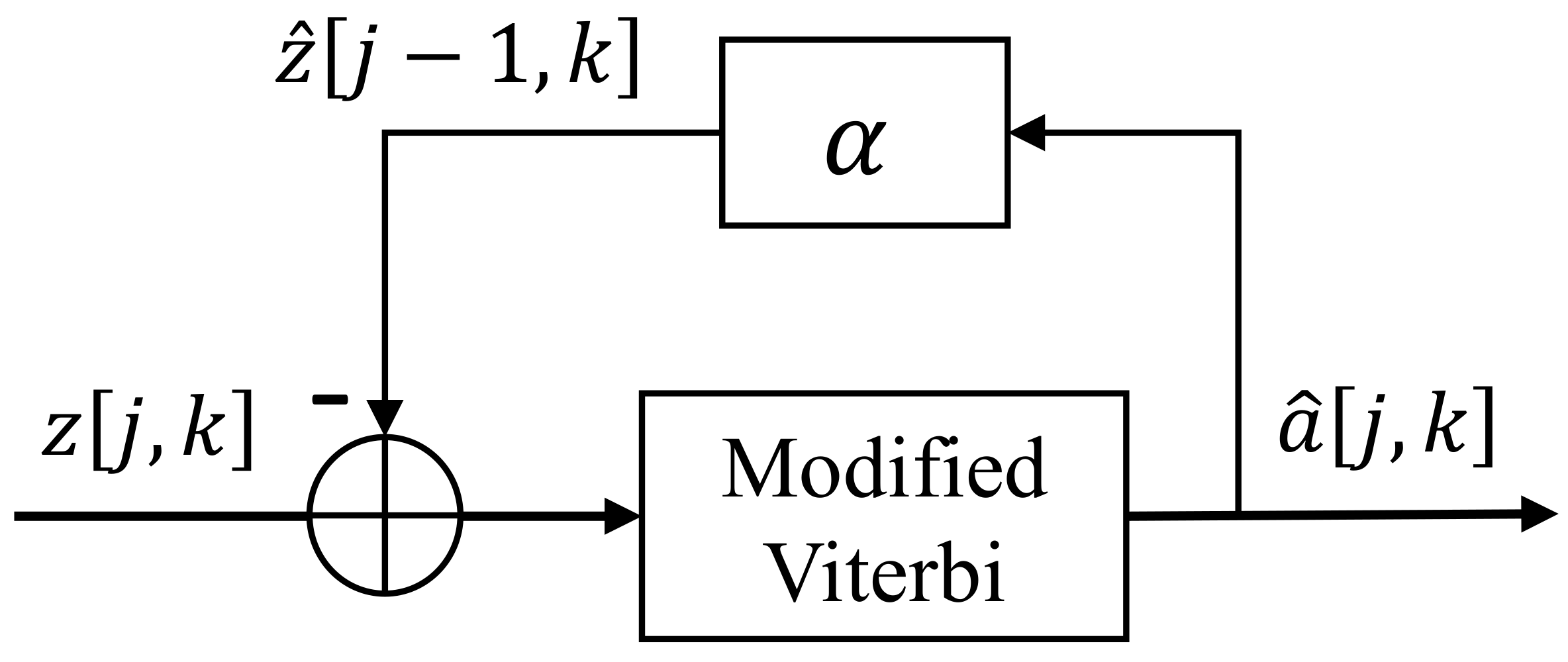
3.3. Three-Way GPR Target and Three-Way MVA with Feedback

In this section, we consider a channel represented by the following matrix form H:

$$H=\left[\begin{array}{ccc}{h}_{-1,-1}& h_{-1,0}& h_{-1,1}\\ h_{0,-1}& h_{0,0}& h_{0,1}\\ h_{1,-1}& h_{1,0}& h_{1,1}\end{array}\right]$$

(43)

The channel output (in the case of zero TMR) can be written as listed below, where * denotes convolution, the h_0,k coefficients are [h_0,−1, h_0,0, h_0,1], the h_−1,k coefficients are [h_−1,−1, h_−1,0, h_−1,1], and the h_1,k coefficients are [h_{1, −1}, h_1,0 h_1,1]:

$$\begin{array}{ll}y[j,k]=& a[j,k]*h_{0,k}\\ & +a[j-1,k]*h_{-1,k}+a[j+1,k]*h_{1,k}+n[j,k]\end{array}$$

(44)

The channel coefficients at the edges of H (i.e., h_−1,−1, h_−1,1, h_1,−1, and h_1,1) often have very small values. Similarly, for the equalizer, the interference coefficients at the edge can be zero (h_−1,−1, h_−1,1, h_1,−1, h_1,1 $\approx$ 0). Therefore, we can rewrite the output of the channel as follows:

$$\begin{array}{ll}y[j,k]\approx & a[j,k]*h_{0,k}\\ & +a[j-1,k]h_{-1,0}+a[j+1,k]h_{1,0}+n[j,k]\end{array}$$

(45)

In our proposed system, we use a three-way GPR target with the matrix form in (46) or (47). These targets are achieved when applying (40)–(42) with the appropriate constraints. The reason we did not choose a two-way GPR target is that it ignores the ITI information. Meanwhile, the four-way GPR target would create a large alias, which degrades the performance. We will explain this based on simulations in Section 4.

If the TMR effect is $+{\Delta }_{off}$, we use the form in (46). If the TMR effect is $-{\Delta }_{off}$, we use the form in (47). In other words, based on g_−1,0 and g_1,0, we choose the form in (46) if g_−1,0 $\ge$ g_1,0 (${\alpha }_1\ge {\alpha }_2$) and we choose the form in (47) if g_−1,0 < g_1,0 (${\alpha }_1<{\alpha }_2$). In this analysis, we assume the TMR effect is $+{\Delta }_{off}.$ The analysis is similar when the TMR effect is $-{\Delta }_{off}$.

$$\mathbf{G}=\left[\begin{array}{ccc}0& {\alpha }_1& 0\\ r& 1& r\\ 0& 0& 0\end{array}\right]$$

(46)

$$\mathbf{G}=\left[\begin{array}{ccc}0& 0& 0\\ r& 1& r\\ 0& {\alpha }_2& 0\end{array}\right]$$

(47)

The output signal d_u[j,k] of the GPR target is expressed as follows:

$$d_u[j,k]=a[j,k]*g_{0,k}+a[j-1,k]{\alpha }_1$$

(48)

where g_0,k coefficients are [r 1 r].

After performing the minimum mean square error (MMSE) algorithm, the output signal of equalizer z[j,k] will be close to the output signal of the GPR target.

$$z[j,k]\approx d_u[j,k]$$

(49)

We can rewrite (49) as follows:

$$y[j,k]*F=a[j,k]*g_{0,k}+a[j-1,k]{\alpha }_1+v\left[j,k\right]$$

(50)

where v[j,k] is the difference between z[j,k] and d_u[j,k]. To increase the accuracy of the expression in (50), we must accurately estimate component v[j,k]. To estimate v[j,k], we will utilize Equations (45) and (48). The ISI component a[j,k]*h_0,k in (45) is represented as a[j,k]*g_0,k in (48), and the ITI component a[j−1,k]h_-1,0 in (45) is converted to a[j−1,k]${\alpha }_1$ in (48). Ideally, the remaining components, a[j+1,k]h_1,0 and n[j,k] in (45), can be suppressed to zero. However, in practice, these components are not zero. In other words, v[j,k] includes the ITI component a[j+1,k] and the noise component n[j,k]. Thus,

$$v[j,k]\approx \epsilon a[j+1,k]+\beta n\left[j,k\right]$$

(51)

Alternatively, we can disregard $\beta$n[j,k], which is relatively small ($\beta \approx$0). Using (51), we replace v[j,k] in (50).

$$y[j,k]*F\approx a[j,k]*g_{0,k}+a[j-1,k]{\alpha }_1+a[j+1,k]\epsilon$$

(52)

For the a[j−1,k]${\alpha }_1$ term, we design a feedback path with a factor of ${\alpha }_1$ to eliminate this component from detection. For a[j+1,k]$\epsilon$, we exploit three-way MVA detection. As a[j+1,k] has a value of {−1,1}, the $\epsilon$ coefficient is added to and subtracted from each branch in the trellis diagram similar to the three-way MVA. (Finding the $\epsilon$ coefficient is presented in Section 4.) This is referred to as the three-way MVA with feedback detection and shown in Figure 8. Our proposed method is summary as Algorithm 1. To easier visualization, we present Algorithm 1 in the Figure 9.

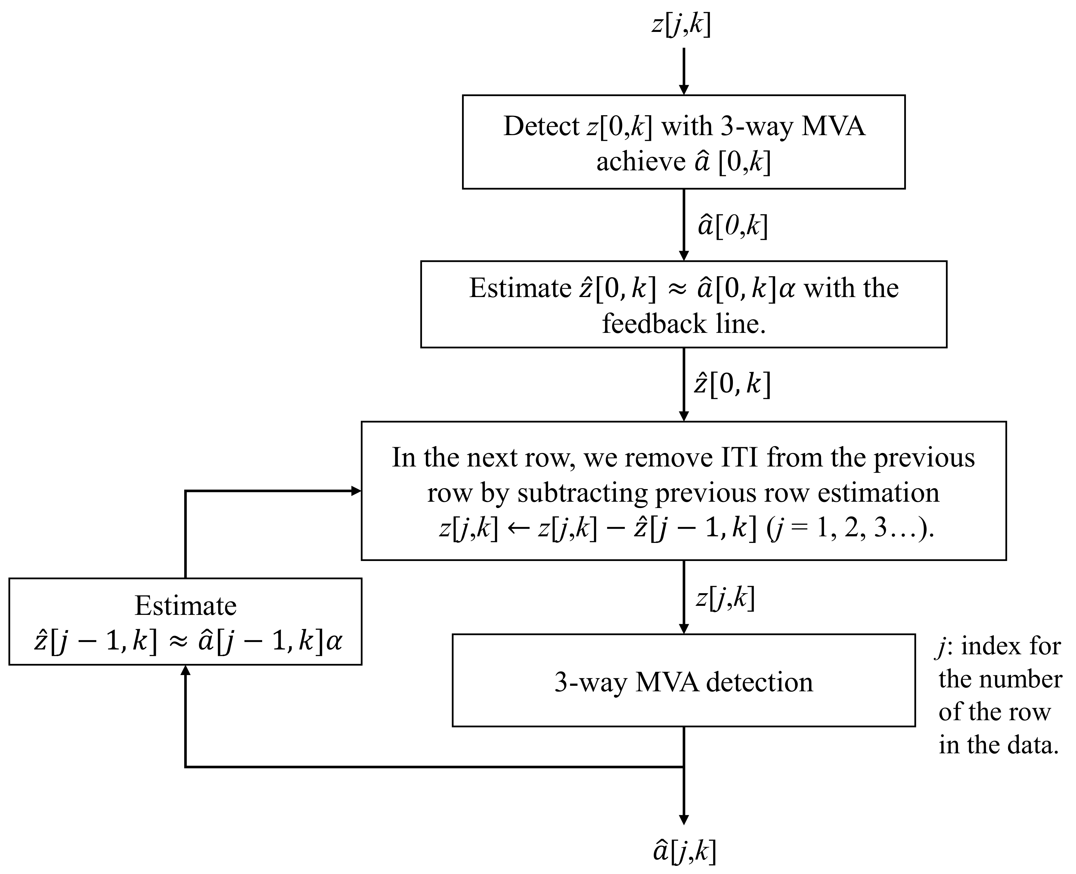
Algorithm 1 Detection procedure of three-way MVA with feedback

Input: Received data $z\left[j,k\right]$. Output: Estimation of original signal $\widehat{a}$[j,k]. 1: Detect the first row of $z\left[j,k\right]$ using a three-way MVA. 2:$j=2$. 3: while$$$\le$ number of rows do 4: Compute $\widehat{z}\left[j-1,k\right]\leftarrow \widehat{a}\left[j-1,k\right]\alpha$.   ($\alpha$ is known from the estimated target.) 5: Calculate $z\left[j,k\right]\leftarrow z\left[j,k\right]-\widehat{z}\left[j-1,k\right]$. 6: Detect $z\left[j,k\right]$ using a three-way MVA. 7:$j\leftarrow j+1$. 8: end while 9: Return $\widehat{a}$[j,k].

4. Simulation Results and Discussion

In this section, we simulated the model as shown in Figure 7. The original signal u[k] $\in$ {0,1} with dimension 1 $\times$ 1,440,000 is converted into a 2D signal a[j,k] $\in$ {−1,1} with dimensions of 1200 $\times$ 1200 by modulation, which is also the size of a data page. Input data a[j,k] pass through the BPMR channel with AWGN. The output of channel y[j,k] becomes the input to a 2D equalizer. We used the 2D equalizer with dimensions 5 $\times$ 5; the equalizer coefficients and the GPR target were estimated by calculating the error signal e[j,k] and applying the MMSE algorithm [20]. Then, the output of equalizer z[j,k] is passed through our detection scheme. Finally, the output $\widehat{a}$[j,k] from the detection scheme is demodulated to obtain $\widehat{u}$[k]. In this paper, we define the channel signal-to-noise ratio (SNR) as 10log₁₀(1/${\sigma }^2$), where ${\sigma }^2$ is the AWGN power. In this experiment, we simulated 10 pages of sample data and an AD of 3 Tb/in² (0.465 Tb/cm²) (T_x = T_z = 14.5 nm) [9]. Our program is built in Matlab R2018a. The coefficients used in the channel simulation are as follows:

$$H=\left[\begin{array}{ccc}0.0824& 0.3876& 0.0824\\ 0.2125& 1& 0.2125\\ 0.0824& 0.3876& 0.0824\end{array}\right]$$

(53)

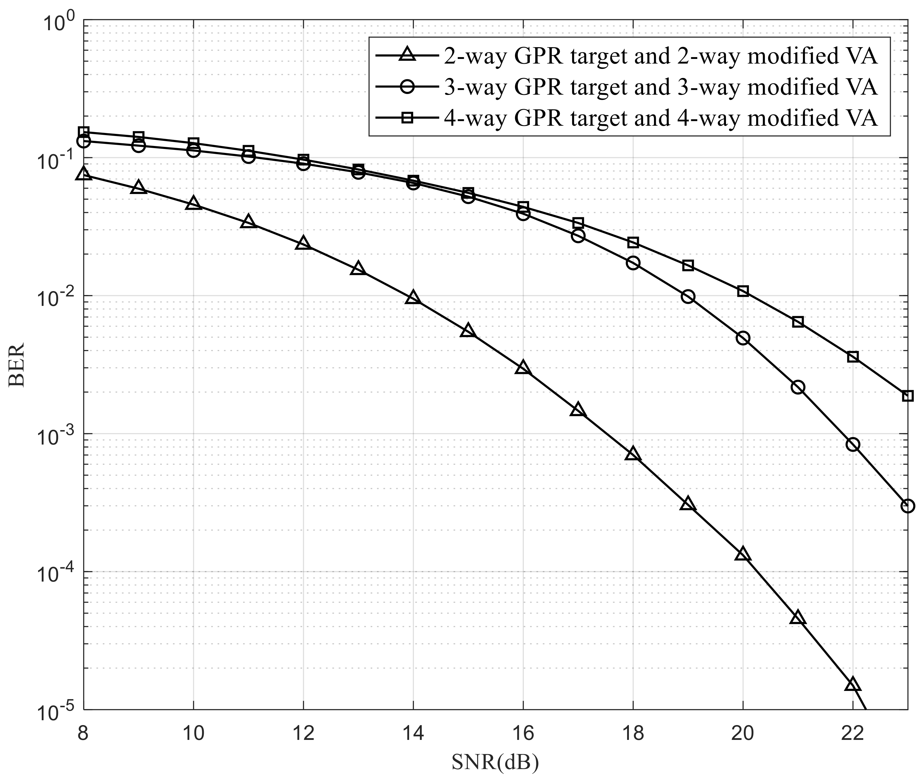
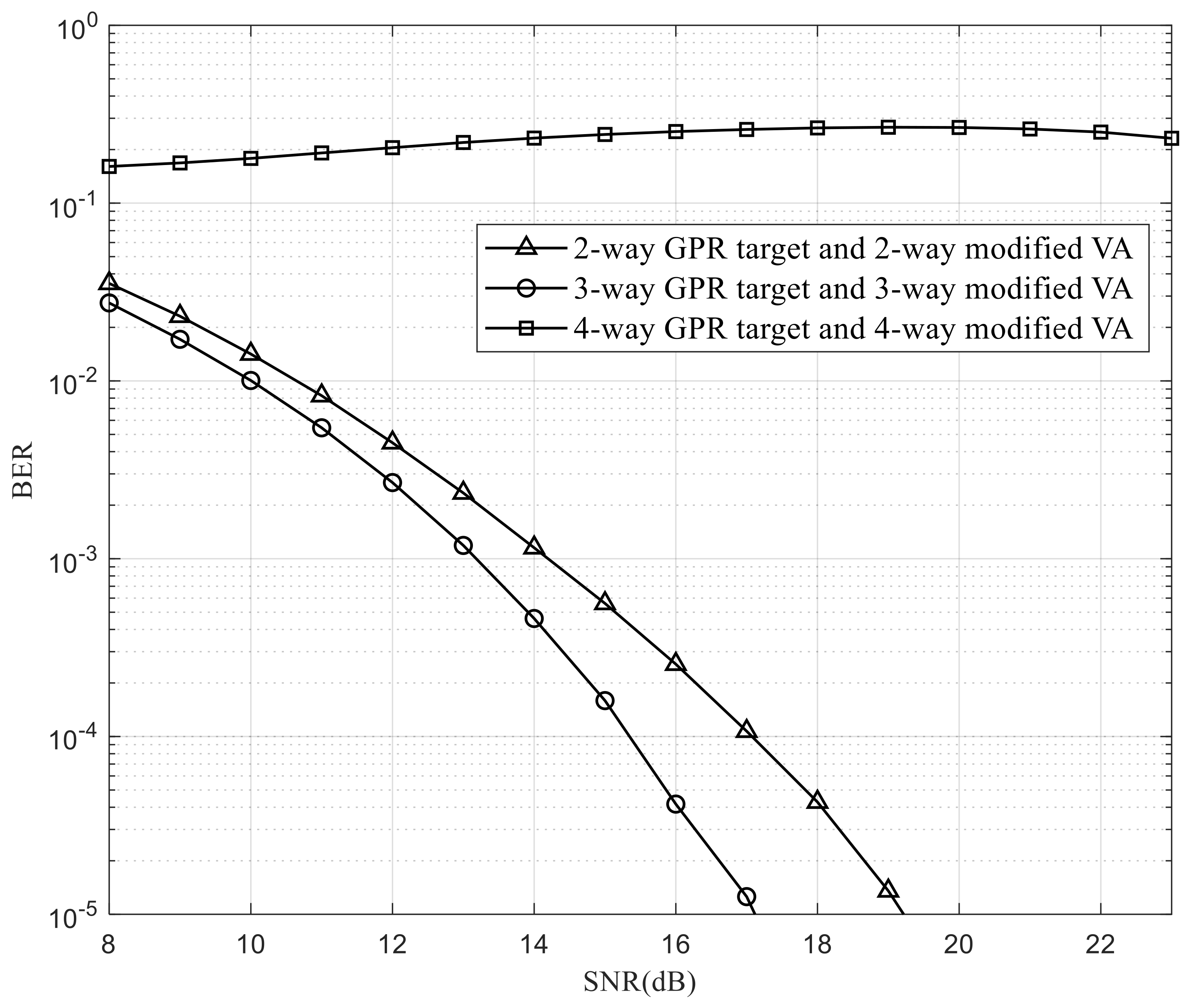
4.1. N-Way GPR Target and N-Way Detection

Figure 10 shows the BER performances for the 2, 3, and 4-way GPR target and its associated 2, 3, and 4-way MVA, respectively. In this experiment, we did not use the feedback path, and the $\epsilon$ coefficient for the N-way MVA was set to the GPR target coefficient such that $\epsilon$ = max (${\alpha }_1,{\alpha }_2$), which is the ITI coefficient from the estimated GPR target. We found that the two-way method, which corresponds to the conventional VA algorithm, achieved the best BER performance. This shows that our signal had additional ITI information when using the three and four-way GPR targets. When the three and four-way MVA were used by themselves, we were not able to take full advantage of the ITI information. For the two-way GPR target, there was no ITI information, whereas for the four-way GPR target, there was too much ITI information, which resulted in a large alias. Therefore, we chose a three-way GPR target with a three-way MVA so that our model would be able to utilize the ITI information in the detection process.

In addition, the accuracy of the detection of the first row is very important owing to the addition of a feedback path in the model. If the first row has many errors, these errors will be propagated through to the next row of the algorithm. Therefore, we monitored the accuracy of the detection of the first rows in all data pages by calculating the BER performance for the first rows on each N-way GPR target and N-way MVA method. In other words, we take the first row of data in each page, then we apply the 2,3,4-way GPR and 2,3,4-way MVA. The results are shown in Figure 11. The three-way GPR target and three-way MVA achieved the best BER performance. This is because the data in the first row are affected by three-way interference. Consequently, the three-way GPR target and three-way MVA were well suited for this condition. Unlike the two-way GPR target, we were able to extract all ITI with the three-way GPR target. Meanwhile, the four-way GPR target and four-way MVA did not appear to affect the BER performance. This is due to the alias effect.

Figure 12 shows that the output values of the trellis are separated into two parts. One part is less than zero, whereas the other is greater than zero. However, if r or p is large enough, these components may be swapped. For instance, when −1 + 2r + p originates from the negative side, there is a high chance of crossover to the positive side.

Table 1. Effect of r and p coefficient for two-way GPR target.

SNR	r	p	−1 + 2r + p
8 dB	0.2130	0	−0.5740
9 dB	0.2248	0	−0.5504
10 dB	0.2363	0	−0.5274
11 dB	0.2471	0	−0.5058
12 dB	0.2565	0	−0.4870
13 dB	0.2642	0	−0.4716
14 dB	0.2698	0	−0.4604
15 dB	0.2730	0	−0.4540
16 dB	0.2735	0	−0.4530
17 dB	0.2713	0	−0.4574
18 dB	0.2663	0	−0.4674
19 dB	0.2585	0	−0.4830
20 dB	0.2481	0	−0.5038
21 dB	0.2353	0	−0.5294
22 dB	0.2206	0	−0.5588
23 dB	0.2043	0	−0.5914

,

Table 2. Effect of r and p coefficient for three-way GPR target.

SNR	r	p	−1 + 2r + p
8 dB	0.1769	0.5275	−0.1187
9 dB	0.1786	0.5458	−0.0970
10 dB	0.1799	0.5613	−0.0789
11 dB	0.1809	0.5741	−0.0641
12 dB	0.1813	0.5844	−0.0530
13 dB	0.1812	0.5922	−0.0454
14 dB	0.1805	0.5977	−0.0413
15 dB	0.1791	0.6010	−0.0408
16 dB	0.1768	0.6025	−0.0439
17 dB	0.1736	0.6023	−0.0505
18 dB	0.1694	0.6007	−0.0605
19 dB	0.1641	0.5978	−0.0740
20 dB	0.1577	0.5941	−0.0905
21 dB	0.1502	0.5896	−0.1100
22 dB	0.1417	0.5847	−0.1319
23 dB	0.1325	0.5795	−0.1555

and

Table 3. Effect of r and p coefficient for four-way GPR target.

SNR	r	p	−1 + 2r + p
8 dB	0.1533	0.8725	0.1791
9 dB	0.1498	0.8867	0.1863
10 dB	0.1462	0.8972	0.1896
11 dB	0.1428	0.9044	0.1900
12 dB	0.1396	0.9085	0.1877
13 dB	0.1367	0.9099	0.1833
14 dB	0.1340	0.9089	0.1769
15 dB	0.1315	0.9058	0.1688
16 dB	0.1289	0.9010	0.1588
17 dB	0.1262	0.8946	0.1470
18 dB	0.1232	0.8871	0.1335
19 dB	0.1198	0.8787	0.1183
20 dB	0.1158	0.8697	0.1013
21 dB	0.1111	0.8604	0.0826
22 dB	0.1058	0.8511	0.0627
23 dB	0.0999	0.8420	0.0418

show the r and p values in the simulation when p = 0 for two-way GPR target, p = $\epsilon$ for three-way GPR target, and p = 2$\epsilon$ for four-way GPR target, respectively; $\epsilon$ is the ITI factor for the GPR target.

Based on the results, the four-way GPR target has the largest alias due to the overlap of the lower branches to the negative side and vice versa. In addition, as the data in the first row are affected by three-way interference, the three-way GPR target and three-way MVA was the most suitable scheme.

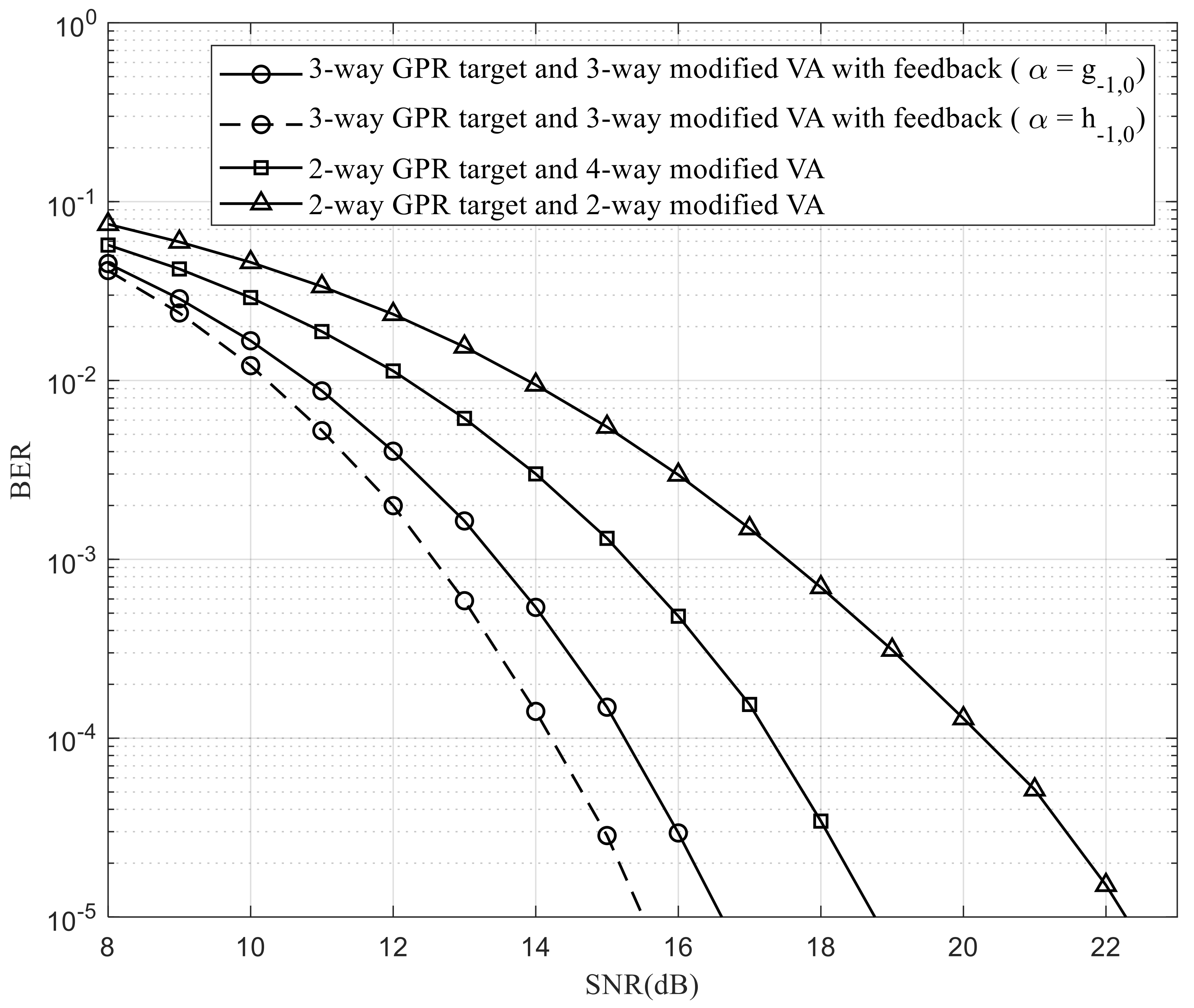
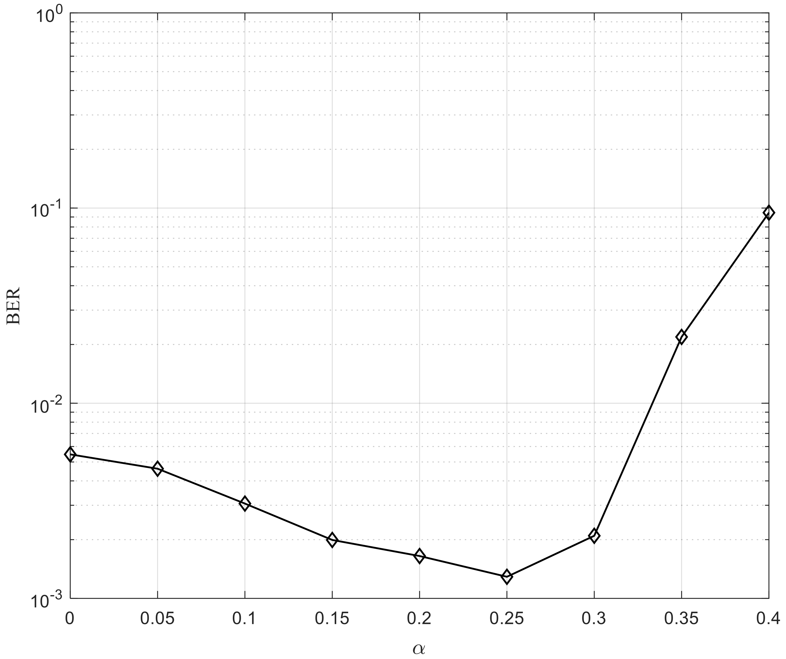
4.2. The Proposed Model

In the next experiment, we compared our proposed model to the MVA. To implement the MVA [12], we had to first determine the interference coefficient ${\epsilon }_{VA}$. Here, we fixed SNR = 15 dB and simulated the BER performance according to ${\epsilon }_{VA}$. Based on the results in Figure 13, we chose ${\epsilon }_{VA}$ = 0.25 for the MVA in [12].

In our algorithm, we will calculate the $\epsilon$ coefficient in (51). As the $\epsilon$ coefficient is the channel’s ITI factor, this means that the coefficient is equal to h_1,0 or h_−1,0. In practice, however, we are not able to determine the values for h_1,0 and h_−1,0. As an alternative, we can use the target factor ${\alpha }_1$ or ${\alpha }_2$ instead of the interference factor. This is possible because the ${\alpha }_1$ or ${\alpha }_2$ in the GPR target is an estimation of h_1,0 or h_−1,0. In addition, this helps in avoiding the simulation for finding the optimum coefficient $\epsilon$ unlike finding ${\epsilon }_{VA}$.

In Figure 14, the two-way GPR target and four-way MVA is the MVA in [12], whereas the two-way GPR target and two-way MVA is the conventional VA in [12]. Based on the results shown in Figure 14, the three-way GPR target and three-way MVA with feedback indicate that our proposed algorithm can be improved with a more accurate estimation of the ITI coefficient. The results also show that our proposed algorithm has an approximately 1 dB gain compared to the MVA at 10⁻⁵ BER.

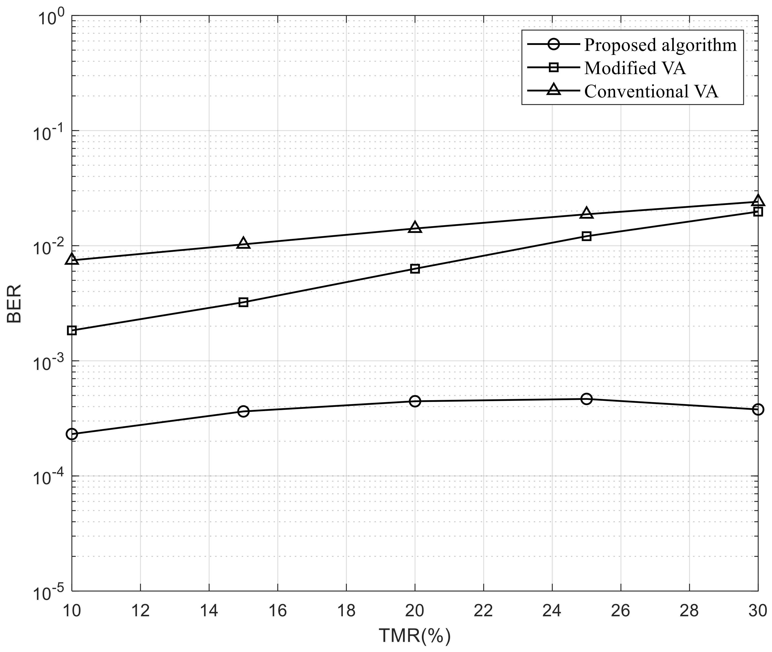
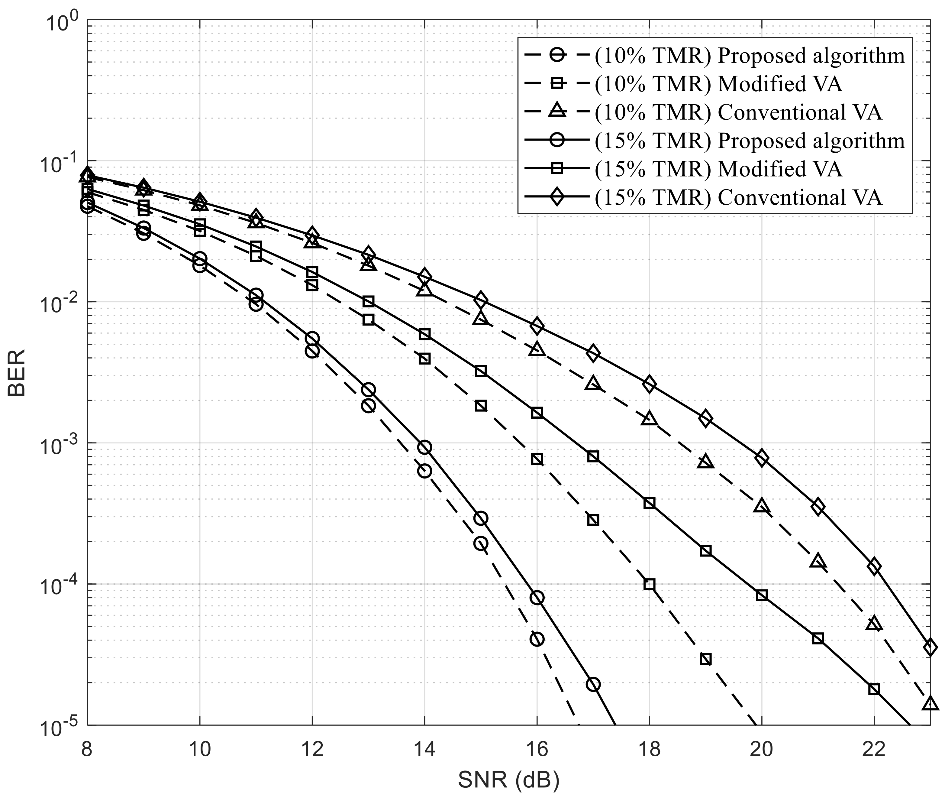
4.3. TMR Effect in BPMR Channel

In this section, we study the effects of TMR. In practice, TMR results in performance degradation; however, it is often difficult to estimate how often it occurs. However, we are able to estimate the ITI with the TMR effect when using the three-way GPR target. In the model, when the TMR is $+{\Delta }_{off}$, the upper interference h_−1,0 is larger than the lower interference h_1,0 (the estimation of GPR results ${\alpha }_1\ge {\alpha }_2)$. Then, the coefficient of the feedback line is ${\alpha }_1$ to reduce ITI. Meanwhile, ${\alpha }_2$ is the estimation of the lower interference h_1,0. Therefore, $\epsilon$ is ${\alpha }_2$ ($\epsilon ={\alpha }_2$). When the TMR is $-{\Delta }_{off}$, the upper ITI h_−1,0 is smaller than the lower one h_1,0 (the estimation of GPR results ${\alpha }_1<{\alpha }_2)$. Then, the coefficient of the feedback line is ${\alpha }_2$ to reduce ITI. Meanwhile, ${\alpha }_1$ is the estimation of the lower ITI h_−1,0. Therefore, $\epsilon$ is ${\alpha }_1$ ($\epsilon ={\alpha }_1$). In general, the feedback coefficient is equal to max $\left({\alpha }_1,{\alpha }_2\right)$ and $\epsilon =\min \left({\alpha }_1,{\alpha }_2\right)$. In our study, we simulated the channel conditions for both 10% and 15% TMR [12].

The results in Figure 15 show that our algorithm was minimally impacted by the variation in TMR as the TMR is reflected on the ITI information and our GPR target estimation is based on the ITI.

In Figure 16, we varied the TMR value from 10 to 30% at SNR = 15 dB. This confirms that our algorithm is not significantly affected by TMR. TMR occurs when the read-head deviates from the main track. This changes the ITI on the receiving signal. The change in ITI is not quantifiable with the conventional scheme. However, with a three-way GPR target, the model is able to estimate the ITI information using ${\alpha }_1$ or ${\alpha }_2$ when TMR occurs. This allows the algorithm to offset the amount of ITI during detection. The proposed scheme is quite resistant to the TMR effect.

4.4. Media Noise in BPMR Channel

To simulate actual conditions, we performed the simulations in the BPMR channel with media noise. First, we tested with 6% and 8% position fluctuation in the simulations [23,24].

In Figure 17, the proposed algorithm was able to achieve a performance gain in the BPMR channel even with 6% and 8% position fluctuation. Then, we increased the position fluctuation further at 15 dB. Figure 18 shows that when the position fluctuation reached 18%, all tested methods had similar BER performance. This means that our proposed algorithm can only withstand a position fluctuation of less than 18%. With position fluctuation, the interference changes randomly. Therefore, the interference coefficient estimator is provided with a lot of randomly changing ITI and ISI information for detection. This makes it possible to improve performance in the BPMR channels even with media noise.

5. Conclusions

In this paper, we presented a detection method that has improved BER performance compared to the MVA [12]. The proposed model is able to achieve an approximately 2 dB gain at 10⁻⁵ dB. With a three-way GPR target, the proposed detection scheme can also improve BER performance when TMR and position fluctuation occur. By employing the feedback line and target, the MVA can estimate the ITI and predict TMR. Due to this, it can choose the solution suitable for the ITI case and TMR case, respectively. With a three-way GPR target, the proposed model also improved the performance against the TMR effect and withstood fluctuations of nearly 18%. The proposed model requires training data to estimate the target before starting the detection of user data. In addition, the proposed detector is based on the MVA, which is fed the ITI information from the GPR and the feedback line. Therefore, the computational complexity is almost the same as conventional Viterbi methods. Finally, we can expect that it is possible to improve the BER performance of the proposed scheme if the MVA detection block is replaced by a BCJR detector with the cost of complexity.

References

1. Thompson, D.A.; Best, J.S. The future of magnetic data storage technology. IBM J. Res. Dev. 2000, 44, 311–322. [Google Scholar] [CrossRef]
2. Jeong, S.; Lee, J. Three typical bit position patterns of bit-patterned media recording. IEEE Magn. Lett. 2018, 9, 1–4. [Google Scholar] [CrossRef]
3. Rottmayer, R.E.; Batra, S.; Buechel, D.; Challener, W.A.; Hohlfeld, J.; Kubota, Y.; Li, L.; Lu, B.; Mihalcea, C.; Mountfield, K.; et al. Heat-assisted magnetic recording. IEEE Trans. Magn. 2006, 42, 2417–2421. [Google Scholar] [CrossRef]
4. Zhu, J.; Zhu, X.; Tang, Y. Microwave assisted magnetic recording. IEEE Trans. Magn. 2008, 44, 125–131. [Google Scholar] [CrossRef]
5. Wood, R.; Williams, M.; Kavcic, A.; Miles, J. The feasibility of magnetic recording at 10 terabits per square inch on conventional media. IEEE Trans. Magn. 2009, 45, 917–923. [Google Scholar] [CrossRef]
6. Honda, N.; Yamakawa, K.; Ouchi, K. Recording simulation of patterned media toward 2 Tb/in2. IEEE Trans. Magn. 2007, 43, 2142–2144. [Google Scholar] [CrossRef]
7. Jeong, S.; Lee, J. Modulation code and multilayer perceptron decoding for bit-patterned media recording. IEEE Magn. Lett. 2020, 11, 1–5. [Google Scholar] [CrossRef]
8. Nguyen, T.A.; Lee, J. Error-correcting 5/6 modulation code for staggered bit-patterned media recording systems. IEEE Magn. Lett. 2019, 10, 1–5. [Google Scholar] [CrossRef]
9. Buajong, C.; Warisarn, C. Improve in bit error rate with a combination of a rate-3/4 modulation code and intertrack interference subtraction for array-reader-based magnetic recording. IEEE Magn. Lett. 2019, 10, 1–5. [Google Scholar] [CrossRef]
10. Kim, J.; Lee, J. Partial response maximum likelihood detections using two-dimensional soft output viterbi algorithm with two-dimensional equalizer for holographic data storage. Jpn. J. Appl. Phys. 2009, 48, 03A003. [Google Scholar] [CrossRef]
11. Kim, J.; Moon, Y.; Lee, J. Iterative two-dimensional soft output viterbi algorithm for patterned media. IEEE Trans. Magn. 2011, 47, 594–597. [Google Scholar] [CrossRef]
12. Nabavi, S.; Kumar, B.V.K.V.; Zhu, J. Modifying viterbi algorithm to mitigate intertrack interference in bit-patterned media. IEEE Trans. Magn. 2007, 43, 2274–2276. [Google Scholar] [CrossRef]
13. Wang, Y.; Kumar, B.V.K.V. Bidirectional decision feedback modified viterbi detection (BD-DFMV) for shingled bit-patterned magnetic recording (BPMR) with 2D sectors and alternating track widths. IEEE J. Sel. Areas Commun. 2016, 34, 2450–2462. [Google Scholar] [CrossRef]
14. Nabavi, S.; Kumar, B.V.K.V.; Bain, J.A. Mitigating the effects of track mis-registration in bit-patterned media. In Proceedings of the IEEE International Conference on Communications (ICC), Bejing, China, 19–23 May 2008; pp. 2061–2065. [Google Scholar] [CrossRef]
15. Wang, Y.; Kumar, B.V.K.V. Improved multitrack detection with hybrid 2-D equalizer and modified viterbi detector. IEEE Trans. Magn. 2017, 53, 1–10. [Google Scholar] [CrossRef]
16. Shi, Y.; Nutter, P.W.; Miles, J.J. Performance evaluation of bit patterned media channels with island size variations. IEEE Trans. Commun. 2013, 61, 228–236. [Google Scholar] [CrossRef]
17. Cheng, T.; Belzer, B.J.; Sivakumar, K. Row-column soft-decision feedback algorithm for two-dimensional intersymbol interference. IEEE Signal Proc. Lett. 2007, 14, 433–436. [Google Scholar] [CrossRef]
18. Zheng, J.; Ma, X.; Guan, Y.L.; Cai, K.; Chan, K.S. Low-complexity iterative row-column soft decision feedback algorithm for 2-d inter-symbol interference channel detection with gaussian approximation. IEEE Trans. Magn. 2013, 49, 4768–4773. [Google Scholar] [CrossRef]
19. Jeong, S.; Kim, J.; Lee, J. Performance of bit-patterned media recording according to island patterns. IEEE Trans. Magn. 2018, 54, 1–4. [Google Scholar] [CrossRef]
20. Nguyen, C.D.; Lee, J. Twin iterative detection for bit-patterned media recording systems. IEEE Trans. Magn. 2017, 53, 1–4. [Google Scholar] [CrossRef]
21. Nabavi, S.; Kumar, B.V.K.V.; Bain, J.A. Two-dimensional pulse response and media noise modeling for bit-patterned media. IEEE Trans. Magn. 2008, 44, 3789–3792. [Google Scholar] [CrossRef]
22. Nabavi, S.; Kumar, B.V.K.V. Two-dimensional generalized partial response equalizer for bit-patterned media. In Proceedings of the IEEE International Conference on Communications, Glasgow, UK, 24–28 June 2007; pp. 6249–6254. [Google Scholar] [CrossRef]
23. Nguyen, T.A.; Lee, J. One-dimensional serial detection using new two-dimensional partial response target modeling for bit-patterned media recording. IEEE Magn. Lett. 2020, 11, 1–5. [Google Scholar] [CrossRef]
24. Nabavi, S.; Kumar, B.V.K.V.; Bain, J.A.; Hogg, C.; Majetich, S.A. Application of image processing to characterize patterning noise in self-assembled nano-masks for bit-patterned media. IEEE Trans. Magn. 2009, 45, 3523–3526. [Google Scholar] [CrossRef]
Figure 1. Data edge of 2D signal.
Applsci 11 00728 g001
Figure 2. Cases of N-way interference.
Applsci 11 00728 g002
Figure 3. Trellis diagram for conventional Viterbi algorithm (VA).
Applsci 11 00728 g003
Figure 4. Trellis diagram for the modified Viterbi algorithm (MVA).
Applsci 11 00728 g004
Figure 5. Coefficient p and N-way detection.
Applsci 11 00728 g005
Figure 6. Alias phenomenon of the output value.
Applsci 11 00728 g006
Figure 7. The proposed system model.
Applsci 11 00728 g007
Figure 8. Three-way MVA with feedback.
Applsci 11 00728 g008
Figure 9. Procedure of three-way MVA with feedback detection.
Applsci 11 00728 g009
Figure 10. Combined N-way generalized partial response (GPR) target and N-way MVA.
Applsci 11 00728 g010
Figure 11. Combined N-way GPR target and N-way MVA for the data in the first row.
Applsci 11 00728 g011
Figure 12. Output values of the trellis diagram converted into number axis.
Applsci 11 00728 g012
Figure 13. Bit error rate (BER) versus ε V A for modified VA.
Applsci 11 00728 g013
Figure 14. BER performance for our proposed algorithm.
Applsci 11 00728 g014
Figure 15. BER versus SNR for 10% and 15% track misregistration (TMR).
Applsci 11 00728 g015
Figure 16. BER versus TMR at 15 dB.
Applsci 11 00728 g016
Figure 17. BER versus SNR for 6% and 8% position fluctuation.
Applsci 11 00728 g017
Figure 18. BER versus fluctuation position from 6% to 18%.
Applsci 11 00728 g018