On the Redundancy in the Rank of Neural Network Parameters and Its Controllability

Abstract

In this paper, we show that parameters of a neural network can have redundancy in their ranks, both theoretically and empirically. When viewed as a function from one space to another, neural networks can exhibit feature correlation and slower training due to this redundancy. Motivated by this, we propose a novel regularization method to reduce the redundancy in the rank of parameters. It is a combination of an objective function that makes the parameter rank-deficient and a dynamic low-rank factorization algorithm that gradually reduces the size of this parameter by fusing linearly dependent vectors together. This regularization-by-pruning approach leads to a neural network with better training dynamics and fewer trainable parameters. We also present experimental results that verify our claims. When applied to a neural network trained to classify images, this method provides statistically significant improvement in accuracy and 7.1 times speedup in terms of number of steps required for training. Furthermore, this approach has the side benefit of reducing the network size, which led to a model with 30.65% fewer trainable parameters.

1. Introduction

Recently, neural networks have shown great success in a wide range of tasks, such as achieving superhuman performance in the game of Go [1] and Atari games [2,3], photo-realistic image synthesis [4], and many natural language processing applications [5,6,7,8,9]. One of the key factors behind these achievements is the huge amount of trainable parameters in the model. For instance, the PG-GAN model [10], which is capable of generating high resolution, photo-realistic faces, has about 46 M parameters. Another example is BERT [6], which is a model with around 340 M trainable parameters. At the time of its release, it achieved state-of-the-art performance in eleven natural language processing tasks.

Since the size of deep neural network models keeps getting larger, it is natural to suspect that not all of the parameters might be necessary to show that level of performance. Indeed, research has shown that features and parameters of a neural network tend to have redundancy [11,12,13]. By analyzing the cause of these redundancies, methods that encourage the model to better utilize its full capacity can be developed. Dropout [14] is one of the most successful and widely used examples, where the coadaptation of neurons was suggested as the cause of redundancy.

In this paper, we provide a theoretical and empirical analysis on a type of network redundancy, which we call the redundancy in the rank of parameters. It is based on a linear algebraic interpretation of parameter matrices, which suggests that the rank of it can be lower than the upper bound. Based on this hypothesis, we propose a novel regularization method that can not only improve the training dynamics of a neural network but also reduce the size of it. This regularization-by-pruning approach consists of a loss function that aims at making the parameter rank deficient, and a dynamic low-rank approximation method that gradually shrinks the size of this parameter by closing the gap between the actual rank and its upper bound.

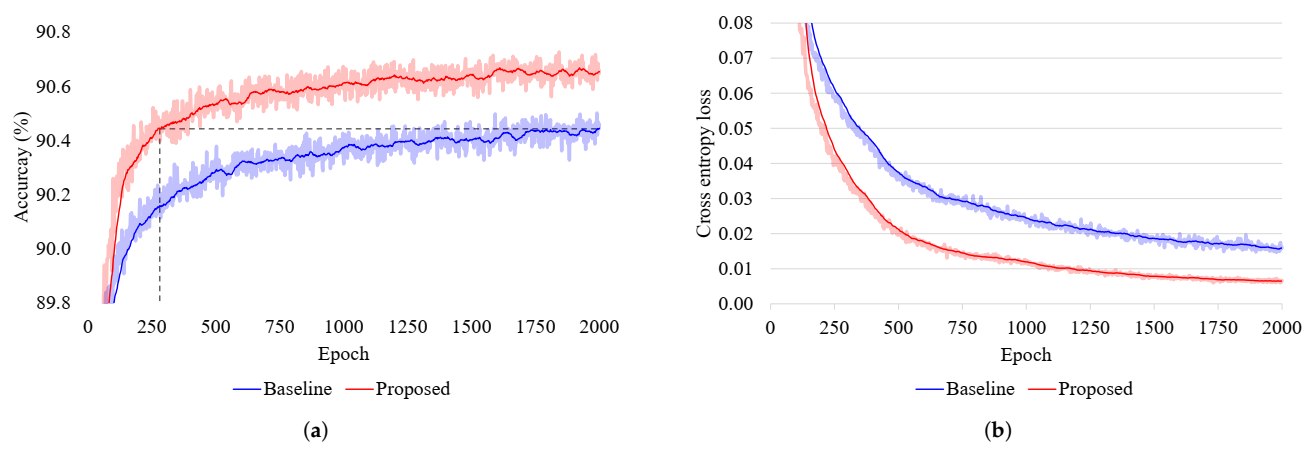
Empirically evaluating this method on an image classification task, we observe that the proposed method leads to a statistically significant accuracy gain of 0.21% and reduces the required number of gradient updates to train the model by a factor of 7. Furthermore, this approach provides the side benefit of reducing 30.65% of the free parameters in the model. Given that these improvements are built on top of other regularization methods such as Dropout, this approach is orthogonal to many other regularization studies and could be used in conjunction with them.

The contributions of this paper can be summarized as follows: (i) We provide theoretical background and analysis regarding this novel type of redundancy, found in the rank of neural network parameters. (ii) We propose a loss function that localizes and identifies redundant parts of a network, in a way that the parameters become rank deficient. (iii) We propose a dynamic low-rank approximation method that lowers the upper bound of the rank of a parameter, by gradually reducing its size. (iv) We provide empirical results that verify our theoretical analysis and claims.

2. Related Work

Many studies have shown that deep neural networks have a lot of redundancy in their parameterization and proposed ways to make better use of the redundant parameters. In the work of Ayinde et al. [15], a measure was proposed to quantify network redundancy, and various architectural choices in designing neural networks were tested using this measure. It is shown that not only the depth and width of the network but also the choice of activation function and initialization method can affect redundancy. Dropout [14] is a widely used regularization method that reduces redundancy by discouraging coadaptation of neurons. Cogswell et al. [16] suggested that the covariance between the activations of a layer is the result of redundancy and designed a loss function that penalizes this. Their method has shown to be effective at reducing overfitting. In Minimum Hyperspherical Energy (MHE) regularization [17], a method that promotes angular diversity of neurons was proposed and was shown to be a strong regularization method. Our method largely falls into this line of work, where the goal is to regularize the network by minimizing redundancy. Unlike the other methods, however, the proposed method has the benefit of reducing the number of trainable parameters.

Low-rank approximation aims to speed up and/or decrease storage footprint of a neural network by representing a parameter tensor with a multiplication of two or more smaller tensors. The work of Sainath et al. [18] was one of the first works to investigate the effectiveness of low-rank matrix factorization in deep neural networks. They used low-rank factorization to compress the final layer of deep neural networks and showed that training speed can be greatly improved with the cost of no or marginal performance lost. In the works of Howard et al. [19] and Kim et al. [20], factorization methods were applied to popular image recognition models to reduce the storage and computation cost, so that they can be ported to mobile devices. GroupReduce [21] is a block-wise low-rank approximation method that utilizes statistical property of word embedding and softmax layers. Since most of the trainable parameters resides in these two matrices, their method has shown great success in compressing large neural language models. In [22], low-rank approximation is utilized to predict the sparsity of the activation in feed-forward neural networks and perform conditional computation to speed up the calculation. The works in [23,24] focused on automatically finding the optimal rank while compressing the kernel of convolutional neural networks via decomposition. DeepTwist [25] proposes to inject noise that simulates weight decomposition during training to mitigate the performance drop caused by the actual decomposition in CNNs. Our work also takes the form of low-rank approximation but with two distinctive properties. First, it does not operate on a trained network and instead can be used during the initial task-specific training. Second, the rank of the factorized matrices does not need to be specified in our approach and is automatically discovered in the process of parameter optimization.

Network pruning is an active research area where the goal is to identify and remove redundant parts of a model. The key to a successful pruning algorithm is an effective method to localize and/or identify the redundant parts of a model. Early works in this literature and some extensions used the Hessian of the loss to determine and remove redundant parts of a neural network [26,27,28]. In [29] applies L2 regularization on the parameters during training and prunes connections with magnitudes below a certain threshold to acquire a sparsified network. This network is then retrained to recover the performance loss. In [11] combines this approach with quantization and Huffman coding to greatly reduce the storage requirement of image recognition models without loss of accuracy. In [30] further extends this work by allowing the threshold parameter to be differentiable so that it can be learned via backpropagation. CLIP-Q [31] performs magnitude-based pruning and quantization in parallel to minimize the side effects of the latter. In [32] also explores magnitude-based pruning but includes a wider range of models and tasks such as LSTMs, language modeling, and neural machine translation. ThiNet [33] greedily removes convolutional filters that has the least contribution to the output of each layer. Some approaches targeted characteristics with more practical implications, such as FLOPs, required for an inference step instead of the number of trainable parameters as the pruning criteria [34,35]. However, pruning processes tend to act adversarially against the model’s performance and require a fine-tuning step to recover the loss [36]. On the other hand, our method works as a regularizer which leads to better accuracy without the requirement of postpruning fine-tuning step.

3. Redundancy in the Rank of Parameters

A neural network layer can be seen as a mapping from one (input) feature space to another (output) feature space. This can be accomplished by combining several transformations. The most typical setting is to map the input feature space to an intermediate space via an affine or linear transformation and map this space to the output feature space with a nonlinearity. This not only applies to fully-connected networks and LSTMs but also to CNNs since in practice convolution operation is reduced to a batch matrix multiplication for efficiency [37]. We will later discuss how this setting can be extended to other neural architectures.

Let $\mathbf{x}= \left[x_1,x_2,\cdots ,x_n\right] \in {\mathbb{R}}^n$ and $\mathbf{y}= \left[y_1,y_2,\cdots ,y_m\right] \in {\mathbb{R}}^m$ be some elements in the input and output feature space of a fully-connected layer, respectively, and $\mathbf{W}= \left[{\mathbf{w}}_1^{\top },{\mathbf{w}}_2^{\top },\cdots ,{\mathbf{w}}_n^{\top }\right] \in {\mathbb{R}}^{m\times n}$ and $\mathbf{b}= \left[b_1,b_2,\cdots ,b_m\right] \in {\mathbb{R}}^m$ be the trainable parameters of it. Then, the mapping from $\mathbf{x}$ to $\mathbf{y}$ using this layer is computed by

$${\displaystyle \widehat{\mathbf{y}}=\sum _{k=1}^n{x}_k{\mathbf{w}}_k+\mathbf{b}}$$

(1)

$$\mathbf{y}=f\left(\widehat{\mathbf{y}}\right),$$

(2)

where $f(·)$ is an element-wise nonlinearity such as the rectifier or sigmoid. Here, $\widehat{\mathbf{y}}$ in (1) can be interpreted as the coordinates of a point in the Cartesian coordinate system, given $\mathbf{x}$ as the affine coordinates over the affine frame with origin $\mathbf{b}$ and basis $\mathbf{W}$ (assuming $\mathbf{W}$ has full rank). Thus, the intermediate feature space is a linear subspace of ${\mathbb{R}}^m$ where its dimension is the rank of $\widehat{\mathbf{W}}=\left[\mathbf{W},{\mathbf{b}}^{\top }\right]$ (i.e., the column space of $\widehat{\mathbf{W}}$).

The key idea is that if $\widehat{\mathbf{W}}$ is rank-deficient, the same mapping can be represented with a smaller $MLI{S}_{strict}(\widehat{\mathbf{W}})$, where $MLI{S}_{strict}\left(\mathbf{A}\right)$ denotes the maximal linearly independent subset of matrix $\mathbf{A}$. However, for fully-connected layers in modern neural architectures, n and m are often in the order of hundreds or thousands [7,38]. In such a high dimension, a set of vectors is almost always linearly independent, especially when they are randomly initialized and optimized towards a certain objective. We argue that even in such a case, $\widehat{\mathbf{W}}$ can be almost linearly dependent, where some vectors in $\widehat{\mathbf{W}}$ can be defined as a linear combination of the other vectors with a small error.

More formally, let $\mathbf{a}=\left[a_1,a_2,\cdots ,a_{n+1}\right]\in {\mathbb{R}}^{n+1}$ be a vector that satisfies

$$\widehat{\mathbf{W}}{\mathbf{a}}^{\top }={\mathbf{0}}^{\top },\mathbf{a}\ne \mathbf{0},$$

(3)

where $\mathbf{0}$ denotes the zero vector. $\widehat{\mathbf{W}}$ is said to be linearly dependent if such $\mathbf{a}$ exists. We propose to introduce a slack variable $\xi \in {\mathbb{R}}^m$ such that

$$\widehat{\mathbf{W}}{\mathbf{a}}^{\top }+{\xi }^{\top }={\mathbf{0}}^{\top },\mathbf{a}\ne \mathbf{0}.$$

(4)

Then, we can find the maximal linearly pseudoindependent subset of a matrix under the condition given by (4). We denote this subset by $MLI{S}_{soft}\left(\mathbf{A}\right)$. The amount of difference that occurs when representing the column space of $\widehat{\mathbf{W}}$ using $MLI{S}_{soft}(\widehat{\mathbf{W}})$ can be controlled by introducing a condition on the slack variable $\xi$, such as ${∥\xi ∥}_2<\tau$. If the rank of $MLI{S}_{soft}(\widehat{\mathbf{W}})$ is smaller than $min(n+1,m)$, which is the upper bound of the rank of $\widehat{\mathbf{W}}$, we can get a lossy mapping from the input feature space to the output feature space with less free parameters. In such case, it can be said that there is redundancy in the rank of $\widehat{\mathbf{W}}$. This implies that there are always at least $|n-m+1|$ linearly dependent vectors along the longer axis, and a square matrix is likely to have the least redundancy in its rank.

When $\widehat{\mathbf{y}}$ is represented with $MLI{S}_{soft}(\widehat{\mathbf{W}})$, its outputs will lie in a lower-dimensional subspace of the original space, spanned by $MLI{S}_{soft}(\widehat{\mathbf{W}})$. However, the dimensionality of the feature space (i.e., outputs of $\mathbf{y}$) can be higher than this subspace due to the nonlinear activation function $f(·)$. This suggests that the null space of $\widehat{\mathbf{W}}$ still could grant some expressive power to this layer.

To close the gap between the upper bound of a parameter and its rank, one can lower the upper bound by shrinking the size of this parameter. By doing so, the same function of this neural network can be approximated with fewer trainable parameters, which leads to a more compact parameter search space.

Another important aspect of the aforementioned interpretation, based on affine frame, is that the input feature space’s entanglement is related to the orthogonality of the basis. Feature space correlation occurs when some change along one basis vector has an effect in the direction of other basis vectors. More formally, let ${\mathbf{v}}_{\mathbf{i}},{\mathbf{v}}_{\mathbf{j}}\in {\mathbb{R}}^n$ be two basis vectors, and $a_i,a_j\in \mathbb{R}$ be their coordinates. Then, the change along the direction of ${\mathbf{v}}_{\mathbf{j}}$ introduced by $a_i{\mathbf{v}}_{\mathbf{i}}$ is given by $a_i{\mathbf{v}}_{\mathbf{i}}·{\mathbf{v}}_{\mathbf{j}}/{\left|{\mathbf{v}}_{\mathbf{j}}\right|}^2{\mathbf{v}}_{\mathbf{j}}$—the orthogonal projection of $a_i{\mathbf{v}}_{\mathbf{i}}$ onto a straight line parallel to ${\mathbf{v}}_{\mathbf{j}}$. Based on this observation, the feature space could be decorrelated by orthogonalizing the basis, but we leave this to a future work.

4. Proposed Method

In this section, we propose a novel method to manipulate the affine frame, based on the theoretical analysis in the previous section. Reducing the size of a neural network parameter based on its rank requires two steps. First, the parameter needs to be made rank deficient, while identifying the linearly dependent vectors in it. Second, we need to find a factorization of this parameter that approximates the original function, by fusing the linearly dependent vectors together.

4.1. Making a Matrix Rank Deficient

We need to find $\mathbf{a}$ that satisfies (4), which in turn identifies vectors that can be represented with a linear combination of the other vectors. However, (4) has infinitely many solutions since for any $\mathbf{a}$ that satisfies (4), $k\mathbf{a}$ where $-1\le k\le 1$ also satisfies it. Furthermore, without explicit control on the interdependence between vectors of $\mathbf{W}$, there is no mean to impose any bounds in $\xi$. To alleviate this issue, we propose a novel objective function that encourages a matrix to be rank deficient.

A matrix is rank deficient when there are linearly dependent vectors, and the most simple form of linear dependence is ${\mathbf{v}}_i=k{\mathbf{v}}_j,k\ne 0\in \mathbb{R}$. This means that ${\mathbf{v}}_i$ and ${\mathbf{v}}_j$ are parallel or opposite to each other. Therefore, an objective function that encourages vectors to be this way can make the matrix rank deficient. Among the family of trigonometric functions, the value of sine function gets closer to zero when the angle between two vectors approach either $0^{\circ }$ or ${180}^{\circ }$. Based on this fact, we build our objective function upon the pairwise squared sine values of a matrix.

Another important factor to consider is the task-specific training objective of the network. When the neural network is optimized for a task, the process can be seen as finding the set of basis vectors of the affine frame that would lead to a desirable feature space transformation. However, minimizing the pairwise squared sine values of a matrix could push these basis vectors to other directions, which in turn can act adversarially against the model’s primary training objective. Our preliminary experiments also supports this hypothesis, where naively minimizing the pairwise squared sine value led to unstable training and inferior performance.

To avoid this side-effect, we design the objective function so that it first chooses a pair of vectors that is the closest to being parallel or opposite, and pushes it further towards this direction. More formally, for a matrix $\mathbf{W}\in {\mathbb{R}}^{m\times n}$, we propose RaRe (Rank Reducing) loss which is defined as follows:

$$RaRe\left(\mathbf{W}\right)=\underset{i}{min}\underset{j\ne i}{min}\left(1-D_{cos}{(i,j,\mathbf{W})}^2\right)$$

(5)

$$D_{cos}(i,j,\mathbf{W})=\frac{{\mathbf{w}}_i·{\mathbf{w}}_j}{∥{\mathbf{w}}_i∥∥{\mathbf{w}}_j∥},$$

(6)

where ${\mathbf{w}}_i$ denotes the ith column of $\mathbf{W}$. Since this loss function affects only a single pair of vectors, it can only reduce the rank of a matrix by 1. This, however, is not a problem since this pair will be merged into a single vector using the method described in the following subsection. An alternative formulation which reduces the squared sine value of k pairs instead of one is possible but performed worse than the proposed form in our preliminary experiments.

4.2. Dynamic Low-Rank Approximation

When a pair of linearly dependent vectors in a matrix is identified, the size of this matrix can be reduced by removing one of the vectors and representing it using the other one. Given the network layer described by (1) and the columns $i,j(i<j)$ as the linearly dependent pair in $\mathbf{W}$, we can create an equivalent function as follows:

$${\mathbf{x}}^{\prime }=\left[\cdots ,x_{i-1},x_{i+1},\cdots ,\frac{(r+1)}{s}{x}_j,\cdots \right]$$

(7)

$$r=\mathrm{\Sigma }{\mathbf{w}}_i/\mathrm{\Sigma }{\mathbf{w}}_j,s=\sqrt{r^2+1}$$

(8)

$${\mathbf{W}}^{\prime }=\left[\cdots ,{\mathbf{w}}_{i-1}^{\top },{\mathbf{w}}_{i+1}^{\top },\cdots ,s{\mathbf{w}}_j^{\top },\cdots \right]$$

(9)

$$\widehat{\mathbf{y}}={\mathbf{W}}^{\prime }{\mathbf{x}\prime }^{\top }+\mathbf{b}.$$

(10)

This can be easily proved by setting ${\mathbf{w}}_i=r{\mathbf{w}}_j$. Since the transformation from $\mathbf{x}$ to ${\mathbf{x}}^{\prime }$ can be implemented with a matrix multiplication, the problem becomes finding the matrices ${\mathbf{W}}^{\prime }\in {\mathbb{R}}^{m\times n^{\prime }}$, $\mathbf{Q}\in {\mathbb{R}}^{n^{\prime }\times n}$ for the original matrix $\mathbf{W}\in {\mathbb{R}}^{m\times n}$, such that ${\mathbf{W}}^{\prime }\mathbf{Q}=\mathbf{W}$ where $n^{\prime }\le n$. This can be accomplished by initializing ${\mathbf{Q}}_0\in {\mathbb{R}}^{n\times n}$ with an identity matrix, and setting the jth row as the weighted sum of the ith and jth row as follows:

$$\mathbf{Q}= \left[\cdots ,{\mathbf{q}}_{i-1},{\mathbf{q}}_{i+1},\cdots ,\left({\mathbf{q}}_i+{\mathbf{q}}_j\times r\right)/s,\cdots \right].$$

(11)

Then, (10) can be rewritten as:

$$\widehat{\mathbf{y}}={\mathbf{W}}^{\prime }\mathbf{Q}{\mathbf{x}}^{\top }+\mathbf{b}.$$

(12)

The reduction process in (8), (9), (11), and (12) can be repeatedly applied whenever a linearly dependent pair of columns is identified.

Similarly, it is possible to fuse pairs of linearly dependent rows. Once linearly dependent rows has been identified after minimizing $RaRe\left({\mathbf{W}}^{\top }\right)$, these rows can be fused by introducing a matrix $\mathbf{P}\in {\mathbb{R}}^{m\times m^{\prime }}$ that satisfies ${\mathbf{PW}}^{\prime }\mathbf{Q}=\mathbf{W}$ where $m^{\prime }\le m$. The process of finding $\mathbf{P}$ and ${\mathbf{W}}^{\prime }$ is almost identical to (9) and (11), except the column operations become row operations and vice versa. When reducing both rows and columns, the vector fusing process along one axis can alter the pairwise angular distances along the other axis. The r and s terms in (9) and (11) are introduced to prevent this issue.

When fusing two vectors with this method, one must choose the vector that is merged to the other one. Since s is always greater than 1, the remaining vector’s magnitude increases. If we choose to keep the vector with greater magnitude, it is more likely to be kept after successive merges and become extremely large. This led to unstable training, so we choose to keep the shorter vector. Even with this precaution, the average magnitude of the vectors tends to increase after multiple merges. Therefore, we utilize L2 weight decay to counter this effect.

Another factor to consider when shrinking the weight parameter is the choice of axis to reduce. Since the upper bound of a $m\times n$ matrix’s rank is $min(m,n)$, the longer axis is likely to have more redundancy. This hypothesis was supported by preliminary experiments, and we design this method to reduce along the longer axis only, keeping its shape close to a square.

Theoretically, this is not an approximation method, since it produces an equivalent function given that the merged pair of vectors are parallel or opposite to each other. However, in practice we find it neither necessary nor efficient to impose such a strict condition. Thus, we approximate the original function by allowing a slight angle between the two vectors. More formally, we fuse ${\mathbf{w}}_i$ and ${\mathbf{w}}_j$ if $1-\left|D_{cos}(i,j)\right|<{\tau }_{cos}$. However, even with a very strict value of ${\tau }_{cos}$, large error could be introduced since large difference in a single dimension would be amortized when calculating the cosine distance in a very high dimensional space. Therefore, we propose to use the Euclidean distance between the two vectors when their magnitudes are equalized, which is calculated as follows:

$$\begin{array}{c}\hfill D_{euc}(i,j,\mathbf{W})= ∥\frac{{\mathbf{w}}_i∥{\mathbf{w}}_j∥}{∥{\mathbf{w}}_i∥}-c{\mathbf{w}}_j∥,\\ \hfill c=\left\{\begin{array}{cc}1\hfill & \mathrm{if}{D}_{cos}(i,j,\mathbf{W})>0\hfill \\ -1\hfill & \mathrm{otherwise}\hfill \end{array}\right..W\end{array}$$

(13)

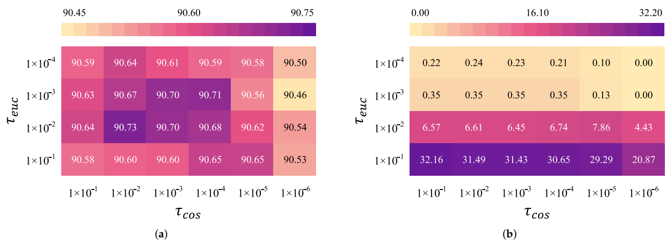
Then we fuse ${\mathbf{w}}_i$ and ${\mathbf{w}}_j$ if $1-\left|D_{cos}(i,j,\mathbf{W})\right|<{\tau }_{cos}$ and $D_{euc}(i,j,\mathbf{W})<{\tau }_{euc}$. The value of ${\tau }_{cos}$ and ${\tau }_{euc}$ can be used to control how aggressively this method reduces the size of a matrix.

4.3. Feature Space Reduction

Even though the feature space could have higher dimensionality than the outputs’ lower-dimensional subspace spanned by $MLI{S}_{soft}(\widehat{\mathbf{W}})$, the feature space can have redundancy in its dimensionality as well. This is due to the fact that many widely-used nonlinear activation functions such as the rectifier or the leaky rectifier are linear almost everywhere. For example, when the rectifier nonlinearity is used, two or more output coordinates in the feature space originated from a fused, single column of $\widehat{\mathbf{W}}$ have linear relationship when they are expected to have the same sign. By exploiting this fact, we reduce the feature space’s dimensionality by fusing these linear coordinates into one coordinate. Since this is not an approximation method, the feature space reduction is a lossless process. When the feature space is reduced, the drop rate of Dropout should be modified to compensate the change, and we linearly decay the rate r as follows:

$$r=\frac{n}{n_0}{r}_0,$$

(14)

where n is the current dimensionality of the feature space, and $n_0,r_0$ are the initial values of $n,r$, respectively.

4.4. Comparison with Low-Rank Approximation

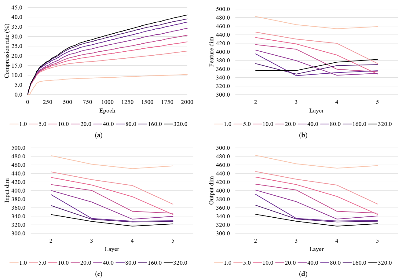
This method can be seen as a form of low-rank approximation. However, there are a few key improvements in this method. First, this process is dynamic, in the sense that the desired rank of the matrix does not need to be predefined. As shown in the experiments section, this leads to different sizes in each layer, allowing the model to have more trainable parameters where needed and to remove parameters that do not affect performance. Similar observations has been made in the automatic structured pruning literature [36,39,40]. Second, in the factorized form ${\mathbf{PW}}^{\prime }\mathbf{Q}$, only ${\mathbf{W}}^{\prime }$ is trainable, while $\mathbf{P}$ and $\mathbf{Q}$ are nontrainable, sparse matrices with only m and n nonzero elements, respectively. This always shrinks the size of the gradient-based parameter search space, which makes the optimization process more efficient and effective. On the contrary, in the case of factorizations where all factorized matrices are trainable, the number of free parameters increases unless $m^{\prime }$ and $n^{\prime }$ becomes small enough to satisfy $m{m}^{\prime }+m^{\prime }{n}^{\prime }+n^{\prime }n<mn$. Third, while most previous low-rank approximation methods focus on factorizing the parameter matrices after the task-specific training is finished, our method is most effective when its applied simultaneously with the training, since it is beneficial to the optimization process. Last but not least, the matrix reduction is a deterministic process that does not require an iterative method.

4.5. Input and Classification Layer

Unlike the hidden layers, the input and classification layers of a neural network serve special purposes and need to be treated differently. The input layer converts the input feature into a dense vector representation. If the size of an input dimension is reduced, part of the input feature is lost, which can lead to degeneration of the performance. In order to prevent this, we do not fuse any columns of the input layer’s parameter.

The classification layer refers to the layer that converts the output feature into logits, which is typically the last layer of a discriminative model. While hidden layers can be seen as functions that map one feature space to another, a classification layer evaluates how close the final output feature is to each class vector [17,41]. Therefore, when two class vectors (i.e., rows) of the classification layer’s parameter get fused, the model loses the ability to distinguish these two classes. Hence, we do not merge any rows in the parameter of the classification layer.

4.6. Frobenius Normalization

Even though the proposed method is orthogonal and can be used with many normalization techniques such as Layer Normalization [42] or Batch Normalization [43], methods that alter the pairwise angular distances between rows or columns could lead to unwanted behavior. Weight Normalization [44] is an example of this case, since the magnitude-decoupling process along one axis of a matrix would alter the pairwise angular distances along the other axis. To alleviate this problem, we propose to use another form of reparameterization called Frobenius Normalization. As its name suggests, the Frobenius norm of a matrix is decoupled via a single trainable scalar, as follows:

$$FN\left(\mathbf{W}\right)=k\mathbf{W}/{∥\mathbf{W}∥}_F\times g,$$

(15)

where k is the initial Frobenius norm of $\mathbf{W}$, and g is the trainable scalar that controls the norm of $\mathbf{W}$, relative to k. Empirically, we find this normalization method to accelerate parameter reduction and stabilize training.

4.7. Training Process

Applying the proposed method to a neural network is simple and straightforward. The detailed training process is shown in Algorithm 1. Given a network with N weight matrices ${\mathbf{W}}_1,{\mathbf{W}}_2,\cdots ,{\mathbf{W}}_N$, each matrix should be replaced with the initial factorized form ${\mathbf{P}}_i{\mathbf{W}}_i^{\prime }{\mathbf{Q}}_i$, where ${\mathbf{W}}_i^{\prime }\in {\mathbb{R}}^{m_i^{\prime }\times n_i^{\prime }}$ is initialized with the values of ${\mathbf{W}}_i$, and ${\mathbf{P}}_i\in {\mathbb{R}}^{m_i\times m_i^{\prime }}$, ${\mathbf{Q}}_i\in {\mathbb{R}}^{n_i^{\prime }\times n_i}$ are initialized with an identity matrix. Then the total RaRe loss for this network is calculated as follows:

$${\mathcal{L}}_{RaRe}=\frac{1}{2c}\sum _{i=1}^N{m}_i^{\prime }{n}_i^{\prime }[RaRe\left({\mathbf{W}}_i^{\prime }\right)+RaRe\left({\mathbf{W}}^{\prime }{\}}_i^{\top }\right)],c=\sum _{i=1}^N{m}_i^{\prime }{n}_i^{\prime }.$$

(16)

Algorithm 1: Training a neural network with Dynamic Low-Rank Approximation.

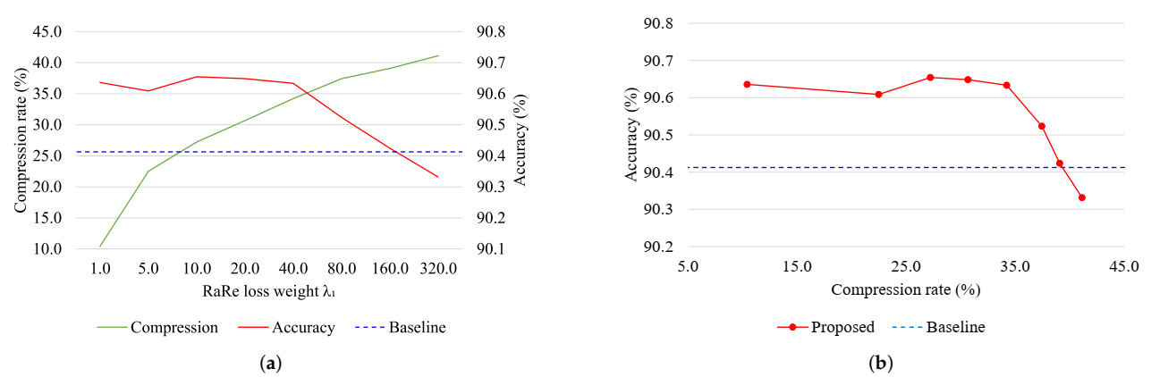
The weighting term $m_i^{\prime }{n}_i^{\prime }$ is introduced to encourage more reduction in larger parameters. As mentioned in the earlier section, the L2 decay loss is calculated as follows:

$${\mathcal{L}}_{L2}=\frac{1}{N}\sum _{i=1}^N{∥{\mathbf{W}}_i^{\prime }∥}_2^2.$$

(17)

These two loss functions are optimized in conjunction with the task specific loss ${\mathcal{L}}_{task}$:

$$\mathcal{L}={\mathcal{L}}_{task}+{\lambda }_1{\mathcal{L}}_{RaRe}+{\lambda }_2{\mathcal{L}}_{L2}.$$

(18)

After each parameter update, the pair of vectors that satisfies (13) is merged using the method described by (8), (9), (11).

Here, we assume that $\mathcal{L}$ is optimized using a gradient-based method, which requires ${\mathcal{L}}_{task}$ to be differentiable w.r.t. the input of the neural network in use. However, this requirement puts minimal restrictions on the type of neural network that can be used, since the use of differentiable neural architecture and loss function (e.g., cross-entropy loss) is the de facto standard in current practice. This setting also mitigates the convergence issue that the nonconvexity of ${\mathcal{L}}_{RaRe}$ might carry. It has been suggested that gradient descent is reasonably effective at optimizing nonconvex functions [45,46], and in some cases the benefits of using nonconvex functions outweigh the absence of convergence guarantee [47]. The empirical results of this study also suggest that ${\mathcal{L}}_{RaRe}$, despite its nonconvexity, improves the stability of the training process (Section 5.2).

4.8. Extending to Other Neural Architectures

So far, we have elaborated our claim and analysis based on the fully-connected network architecture, centered on the parameter matrix. However, the proposed method is independent from most architectural choices such as activation function, batch normalization, and layer normalization. This makes it straightforward to apply this method to architectures that build upon parameter matrices, such as Transformer [7] or Long-Short Term Memory (LSTM) [48].

For other architectures, the concept of rows and columns in the parameter matrix can be generalized using the affine frame interpretation. A column can be seen as the set of elements in a parameter that share the same affine coordinate, and a row is the set of elements that contribute to the same coordinate in the intermediate feature space (i.e., the output space of (1)). In the case of Convolutional Neural Networks (CNN), the weight parameter (i.e., kernel) is typically a 4-dimensional tensor with shape $H\times W\times C_i\times C_o$, where $H,W,C_i,C_o$ are the kernel’s height, width, number of input channels, number of output channels, respectively. Here, a column has the shape of $1\times 1\times 1\times C_o$ and a row has the shape of $H\times W\times C_i\times 1$. Hence, it would be possible to extend this work to reduce the size of a convolution kernel, but we leave this to a future work.

5. Experiments

5.1. Experimental Setup

5.1.1. Models

We use multilayer fully-connected networks to test our hypothesis that reducing the redundancy in the rank of neural network weights could not only reduce the number of free parameters but also help the optimization process. For the baseline model, the network configuration is 784-500-500-500-500-500-10 units which uses the rectifier activation function in the hidden layers and the softmax function in the output layer. All layers, except the output, are regularized using Dropout with 20% drop rate. It is optimized by minimizing ${\mathcal{L}}_{task}$, which is the cross-entropy loss between the model’s prediction and the label. To help training, gradient noise is added as in Neelakantan et al. [49].

To evaluate the proposed method, we minimize $\mathcal{L}$ in (18) and fuse linearly dependent pair of vectors after each update. We use ${\lambda }_1=20.0,{\lambda }_2=0.1$ for all experiments unless otherwise stated. For the values of ${\tau }_{cos}$ and ${\tau }_{euc}$, we find $1e^{-4}$ and $1e^{-1}$ to be good values, respectively, that balances size reduction effectiveness and stable training. Since the dataset has no validation set, the hyperparameters were chosen using 10% of the training data, which were held-out during training.

All models are trained for 2000 epochs using the Adam optimizer [50] with learning rate $1e^{-3}$ and ${\beta }_1=0.9,{\beta }_2=0.999$.

5.1.2. Dataset

We use the Fashion-MNIST dataset [51] to train and evaluate all models. This has the same format (image shape, number of training/test instances, number of classes) as the MNIST dataset but is considered to be more challenging since each image represents a fashion item. No augmentation or preprocessing is performed on the data.

5.2. Results

We use accuracy as our evaluation metric, which is the standard metric in this dataset. Accuracy is defined as the percentage of correct predictions and can be acquired by dividing the number of correctly classified test samples with the total number of test samples. Compression rate is the fraction of parameters removed, compared to the initial number of parameters. To test the statistical significance between different configurations, we train each model 20 times with same hyperparameters but with different random seeds and report the mean and standard deviation.

The change in accuracy and training loss over the course of training is plotted in Figure 1. We also plot the moving average of 20 epochs to highlight the trend. As can be seen, the proposed method achieves the best accuracy of the baseline model, plotted with a dashed line, in just around 280 epochs. This is about $7.1\times$ speedup in terms of number of training steps. Even after this point, the accuracy of this method keeps increasing and reaches to a significantly higher point. The cross entropy loss of the proposed method decreases faster to a lower point compared to the baseline, while also exhibiting less deviation. These results suggest that the proposed method makes the training process more effective and efficient.

In

Table 1. Ablation results, on the Fashion-MNIST test set after training for 2000 epochs. Acc = accuracy, Comp = compression rate, # Param = number of trainable parameters, FLOPs = number of floating point operations for a single inference step, FN = Frobenius normalization, DLRA = dynamic low-rank approximation. P-values are calculated against the baseline model.

	Acc. (%)	p-Value	Comp. (%)	# Param.	FLOPs
Baseline	90.45 ± 0.21	N/A	0.00	1.40 M	2.79 M
+FN	90.51 ± 0.18	1.99 $\times {10}^{-1}$	0.00	1.40 M	2.79 M
+DLRA (${\lambda }_1=20.0$)	90.65 ± 0.15	3.72 $\times {10}^{-4}$	30.65 ± 0.97	0.97 ± 0.01 M	2.09 ± 0.03 M

, the result of an ablation study is summarized. To account for the noise from mini-batched training, all numbers are the average of the last 5 epochs. Please note that we do not show the result of minimizing ${\mathcal{L}}_{RaRe}$ alone, since it would only reduce the pairwise sine value of a single pair of vectors and had almost no effect on the model. When Frobenius Normalization is applied to the baseline model, there is a little improvement in accuracy and decrease in standard deviation. However, the difference is not statistically significant with $p>0.1$. On the other hand, with both Frobenius normalization and dynamic low-rank approximation, we see an average of 2.09% relative error reduction with $p<0.001$. The proposed method is also most reliable in achieving the accuracy, as indicated by the lowest standard deviation. This is more encouraging given the fact that our model has 30.65% less trainable parameters.

There are three hyperparameters that affect the compression—${\tau }_{cos}$, ${\tau }_{euc}$, and ${\lambda }_1$. Overall, we find that ${\lambda }_1$ is more suitable at controlling the compression rate than ${\tau }_{cos}$ or ${\tau }_{euc}$, since the effect of the latter two hyperparameters is less predictable as shown in Figure 2. For this reason, we fix the values of these two hyperparameters and control the model compression using ${\lambda }_1$ in the following experiments. It is worth noting that all combinations of ${\tau }_{cos}$ and ${\tau }_{euc}$ that we have tested still outperformed the baseline model.

To have a better understanding on the effect of compression on the accuracy, the proposed model is trained with different values of ${\lambda }_1$ and the result is plotted in Figure 3 and Figure 4. Again, we measure the average of 20 training runs. Overall, we find that increasing its value leads to a model with fewer trainable parameters as expected. However, this method is less sensitive and ${\lambda }_1$ needs to be changed in an exponential scale to have a noticeable effect. Another thing to note is that a large portion of the reduction in the rank is concentrated on the early phase of training as shown in Figure 4a. We hypothesize that as the training progresses, more parameters become necessary to the model’s objective which makes the rank reduction more difficult.

Intuitively, a model’s performance should decrease as the number of trainable parameters decreases if the model is utilizing all of its weights. However, we find that this is not the case. As can be seen in Figure 3a, the model does not suffer serious degradation in accuracy to the point where 34.22% of the parameters are removed (${\lambda }_1=40.0$). On the other hand, forcing the model to use even fewer parameters leads to a dramatic drop in performance. This can be observed more clearly when the accuracy is plotted as a function of compression rate in Figure 3b. Merely removing 6.91% more parameters from this point results in a model less accurate than the baseline. In addition, the model with 10.41% (${\lambda }_1=1.0$) compression performs worse than the models with 27.22% (${\lambda }_1=10.0$) and 30.65% (${\lambda }_1=20.0$) compression. These results indicate that redundancy in the rank of neural network’s weight can negatively impact the model, and our proposed method is effective at reducing it.

To analyze the amount of redundancy present in each parameter, we summarize the feature, input, and output dimensions after training in Figure 4b–d and

Table 2. Learned model architecture with ${\lambda }_1=20.0$. Init = initial size.

Layer	2	3	4	5	6
Input init.	500	500	500	500	500
Input avg.	413.95	400.20	351.40	346.85	10.00
Input std.	4.92	5.07	13.83	10.01	0.00
Output init.	500	500	500	500	10
Output avg.	414.90	401.20	351.45	347.15	10.00
Output std.	4.97	5.07	13.76	10.30	0.00
Feat. avg.	417.00	406.15	359.30	353.45	10.00
Feat. std.	4.93	5.04	14.63	10.72	0.00

. Overall, all parameters’ shapes become close to a square, due to the reduction process. However, the dimensions of each layer differ while the weighting term in (16) is the same for layers 2 to 5. Similar results were reported in the network pruning literature [36,52] and this suggests that our method is able to effectively identify and remove redundant part of the model. Further, even though the weighting term in (16) of layer 6 is the smallest, its input dimension is reduced most aggressively. Given that this parameter has the highest value of $|n-m|$, this supports our hypothesis that the redundancy is high when the matrix is rank deficient. The dimensionality of the feature space lies in between the initial value and the layer’s output dimension, which is in line with our claim that the feature space can have higher dimension than the output space due to the nonlinear activation function but still has redundancy which is possible to be removed.

6. Conclusions and Future Directions

In this paper, we have provided theoretical and empirical analysis about a novel type of redundancy that can exist in the rank of neural network parameters. Since the actual rank of a parameter can be lower than the upper bound imposed by its size, closing this gap can lead to better training dynamics and fewer trainable parameters. Based on this analysis, we proposed a regularization-by-pruning method that has the side benefit of reducing the size of parameters. This has two parts, where the first part is a loss functions that makes the parameter rank deficient, and the second part is a dynamic low-rank approximation method that reduces the size of this parameter. Empirical analysis of this method shows that it can surpass the baseline accuracy with 7.1 times less training steps and provides an average of 2.09% relative error reduction, on top of Dropout. Furthermore, the proposed model has 30.65% less trainable parameters.

As for future research directions, we plan to investigate deeper about the characteristics of the affine frame of neural networks. Extending the proposed method to other architectures such as CNN and analyzing the effectiveness would be an important step as well. In addition, investigating this method’s pruning effect and combining it with other pruning methods can lead to smaller models, which is essential for resource-limited environments such as mobile devices.