Thermal Analysis of a Concrete Dam Taking into Account Insolation, Shading, Water Level and Spillover

1
Slovenian National Building and Civil Engineering Institute, 1000 Ljubljana, Slovenia
2
Faculty of Civil and Geodetic Engineering, University of Ljubljana, 1000 Ljubljana, Slovenia
*
Author to whom correspondence should be addressed.
Appl. Sci. 2021, 11(2), 705; https://doi.org/10.3390/app11020705
Submission received: 23 December 2020
/
Revised: 8 January 2021
/
Accepted: 10 January 2021
/
Published: 13 January 2021
(This article belongs to the Section Civil Engineering)
Abstract
:Featured Application
Seasonal temperature distributions in concrete dams affect thermal loads, which can cause high stresses in concrete and significantly affect the occurrence and behavior of cracks, as well as displacements (especially in arch-gravity and arch dams).
Abstract
This study presents a procedure for modeling the heat transfer process in a concrete dam, taking into account the time-varying boundary conditions on the upstream and downstream sides of the dam (i.e., the water level of the reservoir, spillover, insolation, and shading) which affect the temperature conditions of the dam. The large concrete arch-gravity Moste Dam (in North West Slovenia) was analyzed, where an automated system for the measurement of concrete and water temperatures, and for the monitoring of meteorological effects, was installed. Thermal analyses (1D and 2D) for non-linear and non-stationary heat conduction through solids were performed using a finite element method (FEM) based program, TeEx, which was complemented by two specially developed programs for determining the effects of convection and insolation, considering also the effect of shading. A 15-day period was analyzed, as well as a period of one year. It was found that the results of the performed analyses fitted in well with the experimentally determined concrete temperature measurements. The results showed that at the insolated side of the dam, the temperature gradient was largest in a very narrow area along the concrete surface, but the temperature did not stabilize shallower than at a depth of about 6 m. As part of the thermal analyses, uncertainty analyses of the results of the calculations were also performed.
1. Introduction
In recent times, the health monitoring of concrete dams has become a topic of great importance and involves monitoring the static and dynamic behavior of large dams [1]. One of the most important parameters that strongly influence the static behavior of concrete dams, especially arch dams, is temperature. For this reason, it is very important to know the seasonal temperature distributions in concrete dams, as they affect the thermal loads, which can cause high stresses in concrete dam structures and significantly affect the occurrence and behavior of cracks, as well as displacements. The effects of climate change and global warming, which may result in a general temperature increase in these structures, need to be considered [2]. Early fundamental research in the field of thermal analysis related to nonlinear and nonstationary heat conduction through a solid, considering suitable boundary conditions, was carried out by Dilger et al. [3] and Carslaw and Jaeger [4], whereas some years later Leger et al. [5,6] presented a methodology based on the finite element method (FEM), which could be used to determine seasonal temperature and stress distributions in concrete gravity dams. Using this methodology, the thermal behavior of concrete dam structures (from arch to gravity) has been much better analyzed, both in the phase of dam design [7,8] as well as in the later phase of monitoring and surveillance of the dam [9,10]. It has been discussed in an increasing number of articles dealing with: stress analysis of concrete structures, which are affected by variable thermal loads [11]; the determination of the periodic temperature field in a concrete dam [12]; the numerical calculation of temperature in a mass concrete [13]; thermal and stress analysis of the discussed roller-compacted concrete dam [14]; and the effect of environmental impacts on thermal stress analysis of the discussed arch concrete dam [15]. Some other authors have discussed the development of new numerical models, such as the model for the analysis of concrete dams due to environmental thermal effects [16], hydrostatic and temperature time-displacement model for concrete dams [17] and hydrostatic seasonal state model for monitoring data analysis of concrete dams [18]. Some others have reported about the sensitivity study of thermal fields in massive structures [19], and about the thermal protection of concrete dams in northern regions [20].
In recent years a large amount of research has been performed in connection with the thermal performance of concrete dams, in which the effects of the changing surrounding conditions were taken into account. Some researchers have focused on detailed studies of displacements dealing with: analysis of concrete dams based on seasonal hydrostatic loading [21]; seasonal thermal displacements of gravity dams, which are located in cold regions [22]; the method of dam deformation due to thermal actions [23]; and correlation between the air temperature and the daily variation of structural response [24]. Other researchers have discussed cracks in the dam structures [25,26], whereas others have analyzed temperature-induced stresses in concrete dams [27,28]. Others again have studied shading effects [29,30] and the effects of solar radiation [31,32], and some reports have discussed temperature fields in the case of super-high arch dams [33,34,35,36].
Some other researchers have recently compared the field monitoring data with the results of numerical analyses of temperature distributions also for other structures (Xia et al. [37] for long-span suspension bridges, Su et al. [38] for supertall structures) and for specific materials (Abid et al. [39] for concrete-encased steel girders).
A literature review of the research on the dam monitoring data analysis methods, which are very important for monitoring the dam safety and where the influence of the environmental variables (e.g., water level, temperature) has been involved, has recently been presented by Li et al. [40].
However, in the above-mentioned articles there seems to be no exhaustive database about the results of temperature measurements over the several decades since the dam’s original construction, or about changing thermal fields in the concrete due to daily and seasonal boundary condition changes.
In this article the authors present a relatively simple procedure which can be used to model the heat transfer process in a concrete dam, taking into account time-varying boundary conditions both on the upstream side of a dam, as the effect of oscillation of the water level of the reservoir, as well as on the downstream, insolated, side, such as the effects of insolation, shading and water spilling over the spillway crest. This procedure was verified at the highest arch-gravity concrete dam in Slovenia.
2. Materials and Methods
2.1. Thermal Analysis of a Concrete Dam
In the case of a concrete dam with incident solar radiation using the effect of shading, a time-varying water level of the reservoir, and occasional spillover, the heat transfer process is shown in Figure 1.
The corresponding equation which relates nonlinear and nonstationary heat conduction in the case of a two-dimensional space and a homogeneous isotropic solid whose thermal conductivity is independent of the temperature [4] is:
where T is the temperature (K); x, y are the Cartesian coordinates (m); ρ is the density (kg/m3); c is the specific heat (J/(kg K)); λ is the thermal conductivity (W/(m K)); and t is the time (s).
The principal types of boundary conditions are:
- Dirichlet or imposed temperature (the defined surface temperature, for instance of the foundation);
- Neumann or imposed heat flux (the defined surface heat flux, that is the absorption of solar radiation considering the effect of shading);
- Robin or convective flux (the heat flux is linearly dependent on the temperature difference between the surface and the ambient temperature, e.g., heat exchange by air convection or by water convection);
- Radiation from the surface of a solid (the heat flux is nonlinearly dependent on the temperature difference between the surface and the ambient temperature).
Heat exchange by convection can be determined by the well-known equation presented by Žvanut et al. [41]:
where qc is the convective flux (W/m2); hc is the convection coefficient (W/m2K); T is the surface temperature of the dam (K); and Ta is the ambient temperature (K).
The effect of radiation was checked and found to be small, so it was neglected. The same was found regarding the effect of cooling of the concrete due to evaporation of absorbed water.
A description of a relatively simple procedure proposed by Dilger et al. [3] for the quite accurate determination of energy flux density due to the absorption of solar radiation is presented by Žvanut et al. [41], where the amount of solar energy absorbed by the body of a system is given by
where qs is the energy flux density of solar radiation absorbed by the solid (W/m2); I is the energy flux density of solar radiation at Earth’s surface (W/m2); a is the solar absorptivity of the surface; and θ is the angle of incidence of Sun’s rays (°);
where Isc is the solar constant (on average 1350 W/m2); and kT is the transparency factor (depends on weather conditions in the atmosphere and the path length of the radiation through the atmosphere);
where kA is factor of altitude H (where H is measured in metres); m is the factor of influence of the relative path length of the radiation (depending on the solar elevation angle βs); and tU is the air pollution factor (between 1.8 for clean air and 9.0 for very polluted air);
The angle of incidence of the Sun’s rays can be presented by
where δ is the declination (i.e., the angle between the equatorial plane and the direction of the Sun; positive towards the North Celestial Pole); Ω is the azimuth of the normal to the plane (measured clockwise from north); α is the angle between the plane and the Earth’s surface; Φ is the geographical latitude; and τ is the hour angle (positive in the morning), which is denoted by
where u is the time of day (in 24-h notation; the hour angle changes at a rate of 15° per hour).
In the case of the vertical plane (α = 90°) Equation (8) can be simplified into
whereas in the case of the horizontal plane (α = 0°) it can be simplified into
where βs is the solar elevation angle.
The solar azimuth angle (αs) defines the direction of the Sun, assuming the north-clockwise convention, and it can be defined by the expression
The heat conduction Equation (1), with appropriately defined boundary conditions, can be solved numerically by the FEM [42]. Such discretization of the model into finite elements results in a system of nonlinear differential equations of the first order. In the case of the searched for time-dependent node temperatures, the system takes the following form:
where K is the thermal conductivity matrix; T is the nodal temperature vector; C is the heat capacity matrix; T,t is the time derivative of temperature; and F is the vector of the external actions.
The left-hand side of Equation (13) and the coefficients depend, in general, on the searched for temperatures (T), whereas the right-hand side is usually also an explicit function of time (t).
2.2. Fieldwork
The large concrete arch-gravity Moste Dam, built in 1952 on the Sava Dolinka River in the north-western part of Slovenia, was analyzed. It is the highest dam in Slovenia, with a structural height of 59.80 m. The dam crest has a length of 72.00 m, whereas the dam volume is 42,000 m3. The spillway crest is at an altitude of 523.50 m. However, the steel gates, which have a height of 1.25 m, increase the effective spillway crest to the altitude of 524.75 m. The dam is located at the north latitude of 46.41°, whereas the azimuth of the symmetrical axis of the downstream side of the Moste Dam is 186°, so that it practically faces south.
An automated system for the measurement of concrete and water temperatures, and for the monitoring of meteorological effects using a mobile automatic weather station (MAWS), was installed on the dam in July 2013. A system for taking automatic measurements of the water level of the reservoir and the height of the water spilling over the spillway crest had been established in 2000.
Before determining the locations of the concrete temperature gauges and the water temperature gauges, preliminary calculations and analyses of the results of the conduction of heat through the concrete structure were performed, as well as a preliminary analysis of the available data regarding the oscillation of the water level of the Moste reservoir for the past 30 years.
Three boreholes were drilled in the dam and six concrete temperature gauges were installed. In the upper borehole on the downstream side of the dam, which was made where the dam surface inclination is 30°, four gauges (TC1 to TC4) were installed at different distances from the dam surface: TC1 at 0.1 m (520.3 m a.s.l.), TC2 at 0.2 m (520.2 m a.s.l.), TC3 at 0.5 m (520.0 m a.s.l.) and TC4 at 1.0 m (519.6 m a.s.l.). In the lower borehole on the downstream side of the dam, which was made where the dam surface inclination is 43°, one gauge (TC6) was placed at a distance of 0.1 m from the dam surface (485.2 m a.s.l.). An additional concrete temperature gauge (TC5) was installed 0.3 m from the dam surface (521.2 m a.s.l.) in a borehole on the upstream side of the dam.
The water temperature measurements were performed using four gauges (TW1 to TW4), placed in a reservoir in a steel pipe, which protected them against floating debris and rushing waters, located at altitudes 519 m, 521 m, 522 m and 523 m. The lowest gauge was installed at a depth that was not affected by the surface zone of changing water temperatures [43], which was confirmed by an additional gauge placed in the reservoir at altitude 511 m.
The measurements of meteorological effects included the following parameters: solar radiation, precipitation, air temperature, wind speed and wind direction. The location of the MAWS, at an altitude 527.65 m, was determined after a detailed visual inspection of the area near the dam, bearing in mind easy accessibility, as few topographical obstacles as possible and low noticeability.
2.3. Procedure for the Thermal Analyses
2.3.1. General
The temperature conditions of the dam were determined by means of the procedure developed for modeling the heat transfer process in concrete dams, taking into account time-varying boundary conditions on both the upstream side of the dam (the effect of the oscillation of the water level of the reservoir) and on the downstream side (the effects of insolation, shading, and water spilling over the spillway crest). Computer programs for the determination of temperature during time, at each node of the finite element mesh, were developed within the programming environments Mathematica [44] and MATLAB [45]. The thermal properties of the mass concrete used in the determining of the temperature conditions of the dam are given in Table 1.
2.3.2. Effect of Spillover
Spilling of water from the reservoir over the spillway crest has an effect on the determination of the parameters of convection (i.e., the temperature and the convection coefficient) and of the heat flux due to insolation, taking into account the effect of shading, on a selected surface, at a given time. In the case that the selected surface is wetted at a certain time due to spillover, the water temperature and water convection coefficient are considered; however, while there is no heat flux due to the insolation. Otherwise, if at a certain time the selected surface is dry (i.e., there is no spillover), the parameters of air convection (i.e., the air temperature and the air convection coefficient) and the measured heat flux due to insolation are taken into account.
During the analyzed year, 1306 h of water spilling over the spillway crest were recorded (from November to May), which is equivalent to 14.9% of the year. The longest period of continuous spillover was recorded between 14 March 2014 at 23:00 and 25 March 2014 at 7:00, and amounted to 249 h, whereas the longest period of continuous spillover at a spillover height of over 5 cm was recorded between 12 May 2014 at 14:00 and 21 May 2014 at 15:00, and amounted to 218 h (Figure 5).
2.3.3. Effect of Shading
In order to investigate the effect of shading (i.e., solar exposure or non-exposure of the observation point on the downstream insolated side of the dam), a method developed by Žvanut et al. [41,46]—based on terrestrial laser scanner measurements of the topography of the wider area of the dam, and of the use of two computer programs (developed within the computing environments Mathematica and MATLAB, respectively)—was applied. Using this approach it is possible to determine—for any selected observation point—the elevation angles of the terrain at different azimuths (i.e., the contour of the terrain), the position of the Sun, and insolation over time. The proposed method has been confirmed as highly reliable in the case of the downstream side of the Moste Dam [46].
2.3.4. Solar Radiation
Back-analyses of the solar radiation were performed for the analyzed period of 15 consecutive clear days in the summer at the location of the MAWS, where the calibrated parameters were obtained [41].
Figure 7 shows the calculated absorbed heat flux due to solar radiation at observation point P1 on the downstream side of the dam in the case of year-round insolation and the measured absorbed heat flux obtained by the measurements of the insolation at the MAWS. The calculated values, which represent the theoretical daily maximums of the heat flux, consistently follow the measured values in the analyzed year, but due to different effects (i.e., cloudiness, partial transparency of the atmosphere) are higher. A greater exception occurs in the winter time, when the measured values are significantly lower than the calculated values in the case of year-round insolation. The main reason for this deviation concerns the difficulties in the insolation measurements at low positions of the Sun (small elevation angles of the Sun and therefore greater lengths of the path of the radiation through the atmosphere) in the winter. The maximum daily maximum (annual maximum) of calculated absorbed heat flux in the case of year-round insolation during the analyzed year was 630 W/m2 in the summer period, whereas the minimum daily maximum of calculated absorbed heat flux was 284 W/m2 in the winter period (the blue spikes show the daily maximums during the year). Figure 7 also shows the zero-values of the heat fluxes of solar radiation during the actual water spilling over the spillway crest (the gaps in the timeline).
3. Results and Discussion
3.1. General
The thermal analyses (1D and 2D) were carried out by using the FEM-based computer program TeEx (written in MATLAB, [47]) which was complemented by two specially formulated programs for determining the effects of convection and insolation, taking into account the effect of shading.
Since the same initial concrete temperatures were not the proper approximation of actual conditions at the beginning of analyses, the following procedure was implemented. The initial concrete temperatures were obtained in such a way that using preliminary initial temperatures of 20 °C, the temperatures after five days (for the 1D analyses) or after one year (for the 2D analyses) were first calculated, and then four repetitions of this period were performed, whereby the respective temperatures at the end of each period were used as the initial values of the next repetition. In order to eliminate the impact of the preliminarily selected initial temperatures, the initial values of the actual calculation were therefore defined as the temperatures calculated at the end of the final repetition.
The 15-days period (Section 3.2.1) and the one year period (Section 3.2.2) were first analyzed using a 1D model, represented by a line perpendicular to the concrete surface, for the instrumented locations of the Moste Dam (Figure 2). In both periods the changeable cloudiness with the effect of shading of the dam surface, and the effect of the varying water level of the reservoir with the occasional spilling of water over the spillway crest were taken into account [48]. The heat flux of the absorbed solar radiation was determined from the results of the MAWS measurements. Secondly, the temperature fields of the Moste Dam, during the year, were determined using a 2D model of the symmetrical cross-section of the complete dam, where all the previously mentioned effects were taken into account (Section 3.3). Thirdly, uncertainty analysis of the calculated temperature field of the Moste Dam on 1 August 2014 at 12:00 was performed, using normally distributed random variables (Section 3.4).
3.2. Effect of Spillover
3.2.1. 15-Days Period
Figure 8, Figure 9, Figure 10 and Figure 11 show the measured and calculated concrete temperatures at three downstream gauges (TC1 and TC4 located in the upper borehole, and TC6 located in the lower borehole), with and without the effect of spillover, and at one upstream gauge (TC5), considering the water level of the reservoir, and also the measured air temperatures (or water temperatures, Figure 10) and the height of spillover during the analyzed 15-days period, from 10 May to 25 May 2014.
It can be seen from Figure 8 and Figure 9 that the calculated concrete temperatures at the downstream gauges TC1 and TC4, when taking into account the effect of spillover, are in very good agreement with the measured concrete temperatures during the whole period (the root mean square error (RMSE) is 1.95 at TC1 and 1.73 at TC4, whereas the mean absolute error (MAE) is 1.39 at TC1 and 1.67 at TC4).
The measured and calculated concrete temperatures at the upstream gauge TC5 (Figure 10), during the period of spillover, or more precisely, during the period when the water level of the reservoir is above the altitude of gauge TC5, are in very good agreement (RMSE is 0.45 and MAE is 0.31).
From Figure 11 it can also be seen that there is very good agreement between the measured and calculated concrete temperatures at gauge TC6, taking into account the effect of spillover, assuming that the height of the spillover must be at least 0.1 m, otherwise the exposed surface of the lower downstream borehole is not wetted (RMSE is 1.28 and MAE is 1.07).
Figure 3 shows the minor amount of spillover (when the height of spillover is less than 0.1 m), where it can be seen that the exposed surface of the upper borehole, with gauges TC1 to TC4, is wetted irrespective of the height of spillover, whereas the exposed surface of the lower borehole, with gauge TC6, is not wetted at a spillover height of less than 0.1 m, since it is located outside of the central cross-section of the dam and therefore not reached by the wetted area of the downstream side of the dam.
The maximum (or minimum) temperature at the specific point in concrete occurs later than the maximum (or minimum) air temperature. This time difference is termed the time lag and depends on the distance from the concrete surface. At a depth of 0.1 m (gauges TC1 and TC6) the time lag was fairly short (at maximum temperatures 1 to 2 h, and at minimum temperatures 3 to 4 h). At a depth of 0.2 m (gauge TC2) the time lag was slightly longer (at maximum temperatures 2 to 3 h, and at minimum temperatures 4 to 5 h). At a depth of 0.3 m (gauge TC5) the time lag at the maximum temperatures was 5 to 6 h, and 6 to 8 h at the minimum temperatures. At a depth of 0.5 m (gauge TC3) the time lag was already 10 to 12 h, and at a depth of 1.0 m (gauge TC4) the time lag was even several days.
3.2.2. One Year Period
Figure 12 and Figure 13 show the measured and calculated concrete temperatures at two of the downstream gauges (TC3 and TC4, located in the upper borehole), with and without the effect of water spilling over the spillway crest, and the height of spillover during the analyzed one year period, from 1 September 2013 to 1 September 2014. It can be seen from these figures that the calculated concrete temperatures at the downstream gauges TC3 and TC4, when considering the effect of spillover, are in very good agreement with the measured concrete temperatures during the whole year (RMSE is 2.50 at TC3 and 2.00 at TC4, whereas MAE is 2.20 at TC3 and 1.84 at TC4).
The annual concrete temperature oscillations for the analyzed year, at gauges TC1 to TC6, as well as the corresponding air (or water) temperature oscillations are shown in Table 2, Table 3, Table 4.
The annual air temperature oscillations at the location of the MAWS were, for the selected period, between −9.5 and 35.6 °C, so their amplitude was 45.1 °C. At gauge TC1, the analyzed annual oscillations were significantly smaller (measured 35.3 °C and calculated 35.9 °C), whereas at gauge TC2 the oscillations were 30.7 and 29.4 °C, respectively. At gauge TC3 the measured annual oscillations were still 24.0 °C, and the calculated oscillations up to 20.6 °C. At gauge TC4 the measured oscillations, over the analyzed annual period, were 18.4 °C, and the corresponding calculated oscillations 16.9 °C.
The annual air temperature oscillations at gauge TW2 were between −1.8 °C and 32.1 °C, so that their amplitude was 33.9 °C, whereas the annual water temperature oscillations were from 2.7 to 19.0 °C and the amplitude was 16.3 °C. However, the annual water temperature oscillations at gauge TW1 were from 2.9 to 16.6 °C, and the amplitude was 13.7 °C. At gauge TC5 the measured annual oscillations were 13.8 °C, and the corresponding calculated oscillations 16.8 °C.
The annual air temperature oscillations close to gauge TC6 were, for the selected period, between −5.8 and 30.1 °C, so that their amplitude was 35.9 °C. The annual concrete temperature oscillations at gauge TC6 were significantly smaller (measured 24.7 °C and calculated 27.5 °C).
3.3. Temperature Field of the Dam
Based on the results of the 2D thermal analyses of the complete dam for the one year period, the temperature fields of the dam during the year were defined, using time periods of two months, starting from 1 October 2013 at 12:00. The temperature fields were plotted using the computer program DIANA [49], where an identical model of the dam as in MATLAB was constructed (i.e., it had the same arrangement and the same denotation of finite elements and nodes), so that when making the temperature fields in DIANA, the results of the thermal analyses calculations from MATLAB (the nodal temperatures at the selected times) were used. Comparing the calculated temperature fields, it was found that the largest gradients in the concrete temperature were recorded in the area close to the surface of the insolated upper part of the downstream side of the dam (Figure 14). This was in summer, when the highest air temperatures occurred and when not much shade was recorded on the downstream side of the dam. For determining the temperature gradient by depth, the two typical cross-sections, A–A and C–C, were chosen (Figure 2 and Figure 14). The four selected points (nodes) coincided with the locations of the temperature gauges.
The concrete temperatures at the two characteristic cross sections in summer (1 August 2014 at 12:00) and in winter (1 February 2014 at 12:00) are presented in Figure 15. It can be seen from this figure that in cross-section A–A at the downstream insolated side of the dam in the summer the calculated temperature from the concrete surface to a depth of 0.2 m was reduced by 9.8 °C, whereas it was reduced at a depth of 1.0 m by 2.4 °C, and by an additional 2.0 °C at a depth of 2.0 m. This suggests that the temperature gradient is largest in a very narrow area along the surface of the concrete. The calculated concrete temperatures in cross-section A–A also indicate that the temperature stabilizes at a depth of about 6.0 m. In the analyzed case, in winter the temperature gradient of the calculated temperatures close to the surface was much smaller, but the strong effect of temperature can be observed up to a depth of 2.0 m. Both in summer and in winter the measured values at three points (at depths of 0.2, 0.5 and 1.0 m) were somewhat higher (by 1.3 to 2.5 °C) than the calculated values.
In cross-section C–C at the upstream side in the summer, when the water level of the reservoir was above the analyzed cross-section, the calculated temperatures from the concrete surface to a depth of 0.3 m were reduced by 2.4 °C, whereas up to a depth of 1.4 m they were reduced by an additional 1.7 °C. This suggests that the temperature gradient is the greatest up to a depth of 0.3 m, and is significantly lower in comparison with the analyzed case in winter (the temperature gradient up to a depth of 0.3 m was 5.8 °C) when the water level of the reservoir was below the analyzed cross-section, so that the concrete surface was exposed to the air. Both in summer and in winter the measured value at a depth of 0.3 m matched the calculated values very well (the differences were 0.1 °C and 0.6 °C, respectively).
3.4. Uncertainty Analysis
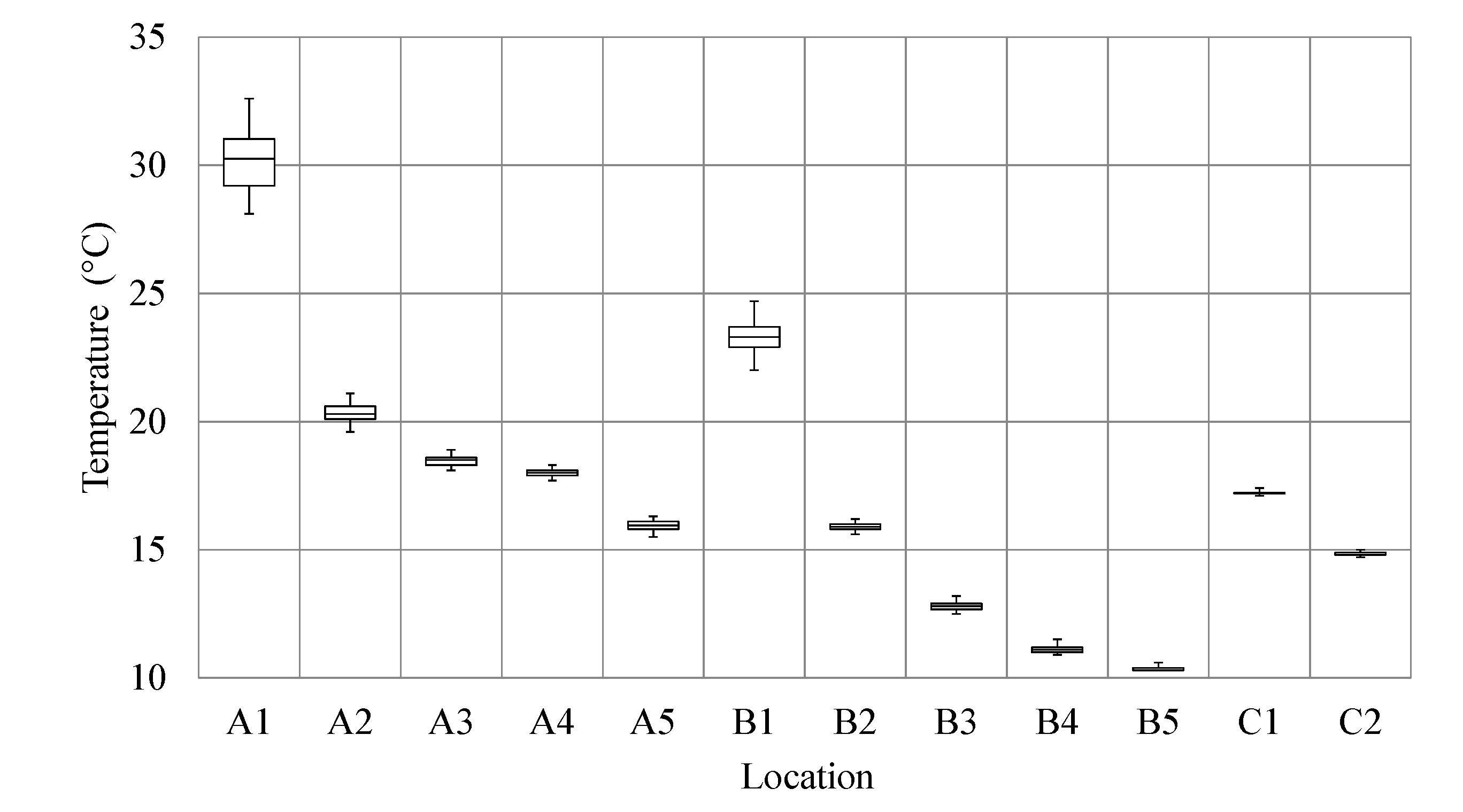
As part of the thermal analyses, uncertainty analyses of the results of the calculations of the concrete temperatures were also performed, where six normally distributed random variables were used to determine the dispersion of the results. Their expected values and standard deviations are given in Table 1. Thermal analysis was carried out for a typical one-month period in the summer (from 1 July 2014 at 12:00 to 1 August 2014 at 12:00), where appropriate temperatures, obtained when calculating the temperature fields of the dam during a one-year period, were considered as the initial temperatures in the analysis (Section 3.3). The concrete temperatures (at 12 selected points on and inside the dam; Figure 2 and Figure 14, Table 5) were analyzed at the end of a period of one month. Sixty repetitions of the calculation (for 60 different combinations of values of six normally distributed random variables), which resulted in 12 different samples, were performed. The calculated values of seven statistics of selected samples of the concrete temperatures are shown in Table 6, whereas the corresponding box-and-whiskers plots are presented in Figure 16.
The maximum average temperature of the 12 samples of populations was obtained at the point A1 (30.24 °C), and the minimum at the point B5 (10.40 °C). The maximum standard deviations were also obtained at point A1 (1.15 °C), whereas the minimum standard deviations were identified at points B5, C1 and C2 (0.08 °C). It was found that the average temperatures of 12 samples of the populations, as compared with the calculated temperatures at the selected points, without considering the point of view of uncertainty, differed by 0.1 °C at four points (A1, A3, A4, B1), whereas at the other eight points there was no difference. The maximum temperature of 12 samples of the populations was obtained at the point A1 (32.6 °C) and the minimum at the point B5 (10.3 °C). At point A1 the maximum interquartile range (1.83 °C) and the maximum range (4.5 °C) were also registered. The minimum interquartile range was calculated for the point C1 (0.03 °C), whereas the minimum range was recorded at the points B5, C1 and C2 (0.3 °C).
4. Conclusions
This article presents a relatively simple procedure for modeling the heat transfer process in a concrete dam, taking into account time-varying boundary conditions on the upstream and downstream sides of the dam (i.e., the water level of the reservoir, spillover, insolation, and shading) which affect the dam’s thermal fields.
The validity of the procedure was verified on the example of the large arch–gravity concrete Moste Dam (the highest such dam in Slovenia), where a sophisticated automated system has recently been installed. This system is used for the measurement of concrete temperatures, as well as to monitor the surrounding conditions (i.e., the water temperatures, the water level of the reservoir, the height of spillover, the air temperature and the solar insolation).
Thermal analyses (1D and 2D) for the analysis of non-linear and non-stationary heat conduction through solids were performed using a FEM-based program, which was complemented by two specially developed programs for determining the effects of boundary conditions during the analyzed 15-day period, as well as during a period of one year. Uncertainty analyses were also carried out to estimate inherent random effect.
It was found that the results of the performed thermal analyses fitted in well with the experimentally determined concrete temperature measurements. The results showed that at the insolated side of the dam, the temperature gradient was largest in a very narrow area along the concrete surface, but the temperature did not stabilize at depths shallower than about 6 m.
The obtained results (i.e., seasonal temperature distributions in the dam) affect the thermal loads, which can cause high tensile stresses in concrete and importantly affect the occurrence and behavior of cracks, as well as displacements; especially in arch dams and arch-gravity dams.
Author Contributions
Conceptualization, P.Ž., G.T. and A.K.; methodology, P.Ž., G.T. and A.K.; software, P.Ž. and G.T.; validation, P.Ž. and G.T.; formal analysis, P.Ž.; investigation, P.Ž., G.T. and A.K.; resources, P.Ž.; data curation, P.Ž.; writing—original draft preparation, P.Ž., G.T. and A.K.; writing—review and editing, P.Ž., G.T. and A.K.; visualization, P.Ž. and G.T.; supervision, P.Ž., G.T. and A.K.; project administration, P.Ž.; funding acquisition, P.Ž. All authors have read and agreed to the published version of the manuscript.
Funding
The presented article is part of research work that was performed within the scope of the first author’s doctoral studies, and was partly funded by the European Union through the European Social Found.
Institutional Review Board Statement
Not applicable.
Informed Consent Statement
Not applicable.
Data Availability Statement
The data presented in this study are available on request from the corresponding author. The data are not publicly available due to the requirements of the company Savske elektrarne Ljubljana Ltd.
Acknowledgments
The authors would like to thank the company Savske elektrarne Ljubljana Ltd., which enabled the field work. The authors would also like to acknowledge the financial support of the Slovenian Research Agency through infrastructure program I0-0032, research program P2-0260 and research project J2-9196.
Conflicts of Interest
The authors declare no conflict of interest.
References
- Bukenya, P.; Moyo, P.; Beushausen, H.; Oosthuizen, C. Health monitoring of concrete dams: A literature review. J. Civ. Struct. Health Monit. 2014, 4, 235–244. [Google Scholar] [CrossRef]
- Santillan, D.; Salete, E.; Toledo, M.A. A methodology for the assessment of the effect of climate change on the thermal-strain-stress behaviour of structures. Eng. Struct. 2015, 92, 123–141. [Google Scholar] [CrossRef]
- Dilger, W.H.; Ghali, A.; Chan, M.; Cheung, M.S.; Maes, M.A. Temperature stresses in composite box girder bridges. J. Struct. Eng. 1983, 109, 1460–1478. [Google Scholar] [CrossRef]
- Carslaw, H.S.; Jaeger, J.C. Conduction of Heat in Solids, 2nd ed.; Oxford University Press: New York, NY, USA, 1986; ISBN 978-0198533689. [Google Scholar]
- Leger, P.; Venturelli, J.; Bhattacharjee, S.S. Seasonal temperature and stress distributions in concrete gravity dams. Part 1: Modelling. Can. J. Civ. Eng. 1993, 20, 999–1017. [Google Scholar] [CrossRef]
- Leger, P.; Venturelli, J.; Bhattacharjee, S.S. Seasonal temperature and stress distributions in concrete gravity dams. Part 2: Behavior. Can. J. Civ. Eng. 1993, 20, 1018–1029. [Google Scholar] [CrossRef]
- U.S. Army Corps of Engineers. Engineering and Design: Arch Dam Design (Engineer Manual EM 1110-2-2201); Military Bookshop: Washington, DC, USA, 1994; ISBN 978-1780397610. [Google Scholar]
- U.S. Army Corps of Engineers. Engineering and Design: Gravity dam design (Engineer manual EM 1110-2-2200); Military Bookshop: Washington, DC, USA, 1995. [Google Scholar]
- International Commission on Large Dams. Automated Dam Monitoring Systems: Guidelines and Case Histories—Bulletin 118; Commission Internationale des Grands Barrages: Paris, France, 2000. [Google Scholar]
- International Commission on Large Dams. Dam Surveillance Guide—Bulletin 158; Commission Internationale des Grands Barrages: Paris, France, 2012. [Google Scholar]
- Saetta, A.; Scotta, R.; Vitaliani, R. Stress analysis of concrete structures subjected to variable thermal loads. J. Struct. Eng. 1995, 121, 446–457. [Google Scholar] [CrossRef]
- Daoud, M.; Galanis, N.; Ballivy, G. Calculation of the periodic temperature field in a concrete dam. Can. J. Civ. Eng. 1997, 24, 772–784. [Google Scholar] [CrossRef]
- Wu, Y.; Luna, R. Numerical implementation of temperature and creep in mass concrete. Finite Elem. Anal. Des. 2001, 37, 97–106. [Google Scholar] [CrossRef]
- Noorzaei, J.; Bayagoob, K.H.; Thanoon, W.A.; Jaafar, M.S. Thermal and stress analysis of Kinta RCC dam. Eng. Struct. 2006, 28, 1795–1802. [Google Scholar] [CrossRef]
- Sheibany, F.; Ghaemian, M. Effects of environmental action on thermal stress analysis of Karaj concrete arch dam. J. Eng. Mech. 2006, 132, 532–544. [Google Scholar] [CrossRef]
- Agullo, L.; Mirambell, E.; Aguado, A. A model for the analysis of concrete dams due to environmental thermal effects. Int. J. Numer. Methods Heat Fluid Flow 1996, 6, 25–36. [Google Scholar] [CrossRef] [Green Version]
- Leger, P.; Leclerc, M. Hydrostatic, temperature, time-displacement model for concrete dams. J. Eng. Mech. 2007, 133, 267–277. [Google Scholar] [CrossRef]
- Li, F.Q.; Wang, Z.Y.; Liu, G.H.; Fu, C.J.; Wang, J.J. Hydrostatic seasonal state model for monitoring data analysis of concrete dams. Struct. Infrastruct. Eng. 2015, 11, 1616–1631. [Google Scholar] [CrossRef]
- Zhang, P.X.; Ayari, M.L.; Robinson, L.C. Role of fundamental heat transfer frequency in the computation of transient thermal fields in massive structures. Can. J. Civ. Eng. 1997, 24, 1059–1065. [Google Scholar] [CrossRef]
- Leger, P.; Cote, M.; Tinawi, R. Thermal protection of concrete dams subjected to freeze—Thaw cycles. Can. J. Civ. Eng. 1995, 22, 588–602. [Google Scholar] [CrossRef]
- Ardito, R.; Maier, G.; Massalongo, G. Diagnostic analysis of concrete dams based on seasonal hydrostatic loading. Eng. Struct. 2008, 30, 3176–3185. [Google Scholar] [CrossRef]
- Leger, P.; Seydou, S. Seasonal thermal displacements of gravity dams located in northern regions. J. Perform. Constr. Facil. 2009, 23, 166–174. [Google Scholar] [CrossRef]
- Xu, B.S.; Liu, B.B.; Zheng, D.J.; Chen, L.; Wu, C.C. Analysis method of thermal dam deformation. Sci. China Technol. Sci. 2012, 55, 1765–1772. [Google Scholar] [CrossRef]
- Mata, J.; de Castro, A.T.; da Costa, J.S. Time-frequency analysis for concrete dam safety control: Correlation between the daily variation of structural response and air temperature. Eng. Struct. 2013, 48, 658–665. [Google Scholar] [CrossRef] [Green Version]
- Malm, R.; Ansell, A. Cracking of concrete buttress dam due to seasonal temperature variation. ACI Struct. J. 2011, 108, 13–22. [Google Scholar]
- Maken, D.D.; Leger, P.; Roth, S.N. Seasonal thermal cracking of concrete dams in northern regions. J. Perform. Constr. Facil. 2014, 28. [Google Scholar] [CrossRef]
- Labibzadeh, M.; Sadrnejad, S.A.; Khajehdezfuly, A. Thermal assessment of Karun-1 Dam. Trends Appl. Sci. Res. 2010, 5, 251–266. [Google Scholar] [CrossRef] [Green Version]
- Santillan, D.; Salete, E.; Toledo, M.A. A new 1D analytical model for computing the thermal field of concrete dams due to the environmental actions. Appl. Therm. Eng. 2015, 85, 160–171. [Google Scholar] [CrossRef]
- Jin, F.; Chen, Z.; Wang, J.T.; Yang, J. Practical procedure for predicting non-uniform temperature on the exposed face of arch dams. Appl. Therm. Eng. 2010, 30, 2146–2156. [Google Scholar] [CrossRef]
- Santillan, D.; Salete, E.; Vicente, D.J.; Toledo, M.A. Treatment of solar radiation by spatial and temporal discretization for modeling the thermal response of arch dams. J. Eng. Mech. 2014, 140, 05014001. [Google Scholar] [CrossRef]
- Mirzabozorg, H.; Hariri-Ardebili, M.A.; Shirkhan, M.; Seyed-Kolbadi, S.M. Mathematical modeling and numerical analysis of thermal distribution in arch dams considering solar radiation effect. Sci. World J. 2014, 597393. [Google Scholar] [CrossRef] [Green Version]
- Liu, H.B.; Liao, X.W.; Chen, Z.H.; Zhang, Q. Thermal behavior of spatial structures under solar irradiation. Appl. Therm. Eng. 2015, 87, 328–335. [Google Scholar] [CrossRef]
- An, G.; Yang, N.; Li, Q.B.; Hu, Y.; Yang, H.T. A simplified method for real-time prediction of temperature in mass concrete at early age. Appl. Sci. 2020, 10, 4451. [Google Scholar] [CrossRef]
- Hu, Y.; Zuo, Z.; Li, Q.B.; Duan, Y.L. Boolean-based surface procedure for the external heat transfer analysis of dams during construction. Math. Probl. Eng. 2013, 175616. [Google Scholar] [CrossRef] [Green Version]
- Liu, Y.; Zhang, G.X.; Zhu, B.F.; Shang, F. Actual working performance assessment of super-high arch dams. J. Perform. Constr. Facil. 2016, 30, 04015011. [Google Scholar] [CrossRef]
- Yin, T.; Li, Q.B.; Hu, Y.; Yu, S.; Liang, G.H. Coupled thermo-hydro-mechanical analysis of valley narrowing deformation of high arch dam: A case study of the Xiluodu project in China. Appl. Sci. 2020, 10, 524. [Google Scholar] [CrossRef] [Green Version]
- Xia, Y.; Chen, B.; Zhou, X.Q.; Xu, Y.L. Field monitoring and numerical analysis of Tsing Ma Suspension Bridge temperature behavior. Struct. Control. Health Monit. 2013, 20, 560–575. [Google Scholar] [CrossRef]
- Su, J.Z.; Xia, Y.; Ni, Y.Q.; Zhou, L.R.; Su, C. Field monitoring and numerical simulation of the thermal actions of a supertall structure. Struct. Control. Health Monit. 2017, 24, e1900. [Google Scholar] [CrossRef]
- Abid, S.R.; Mussa, F.; Taysi, N.; Ozakca, M. Experimental and finite element investigation of temperature distributions in concrete-encased steel girders. Struct. Control. Health Monit. 2018, 25, e2042. [Google Scholar] [CrossRef]
- Li, B.; Yang, J.; Hu, D.X. Dam monitoring data analysis methods: A literature review. Struct. Control. Health Monit. 2020, 27, e2501. [Google Scholar] [CrossRef]
- Žvanut, P.; Turk, G.; Kryžanowski, A. Effects of changing surrounding conditions on the thermal analysis of the Moste concrete dam. J. Perform. Constr. Facil. 2016, 30, 04015029. [Google Scholar] [CrossRef] [Green Version]
- Zienkiewicz, O.C. The Finite Element Method, 3rd ed.; McGraw-Hill: London, UK, 1977; ISBN 978-0070840720. [Google Scholar]
- Bofang, Z. Prediction of water temperature in deep reservoirs. Dam Eng. 1997, 8, 13–25. [Google Scholar]
- Wolfram Mathematica Home Page. Available online: http://www.wolfram.com/mathematica (accessed on 10 August 2020).
- MathWorks MATLAB Home Page. Available online: http://www.mathworks.com/products/matlab (accessed on 11 July 2020).
- Žvanut, P.; Vezočnik, R.; Turk, G.; Ambrožič, T. Determination of the shading of the downstream surface of the Moste concrete dam. Geod. Vestnik 2014, 58, 453–465. [Google Scholar] [CrossRef]
- Ilc, A. Nonlinear Analysis of Massive Concrete at Successive Construction. Ph.D. Thesis, University of Ljubljana, Faculty of Civil and Geodetic Eng., Ljubljana, Slovenia, 2013. [Google Scholar]
- Žvanut, P. Thermal Analysis of Large Arch-Gravity Concrete Dams. Ph.D. Thesis, University of Ljubljana, Faculty of Civil and Geodetic Eng., Ljubljana, Slovenia, 2017. [Google Scholar]
- DIANA FEA Home Page. Available online: https://dianafea.com (accessed on 11 August 2020).
Figure 1.
The heat transfer process in a concrete dam.
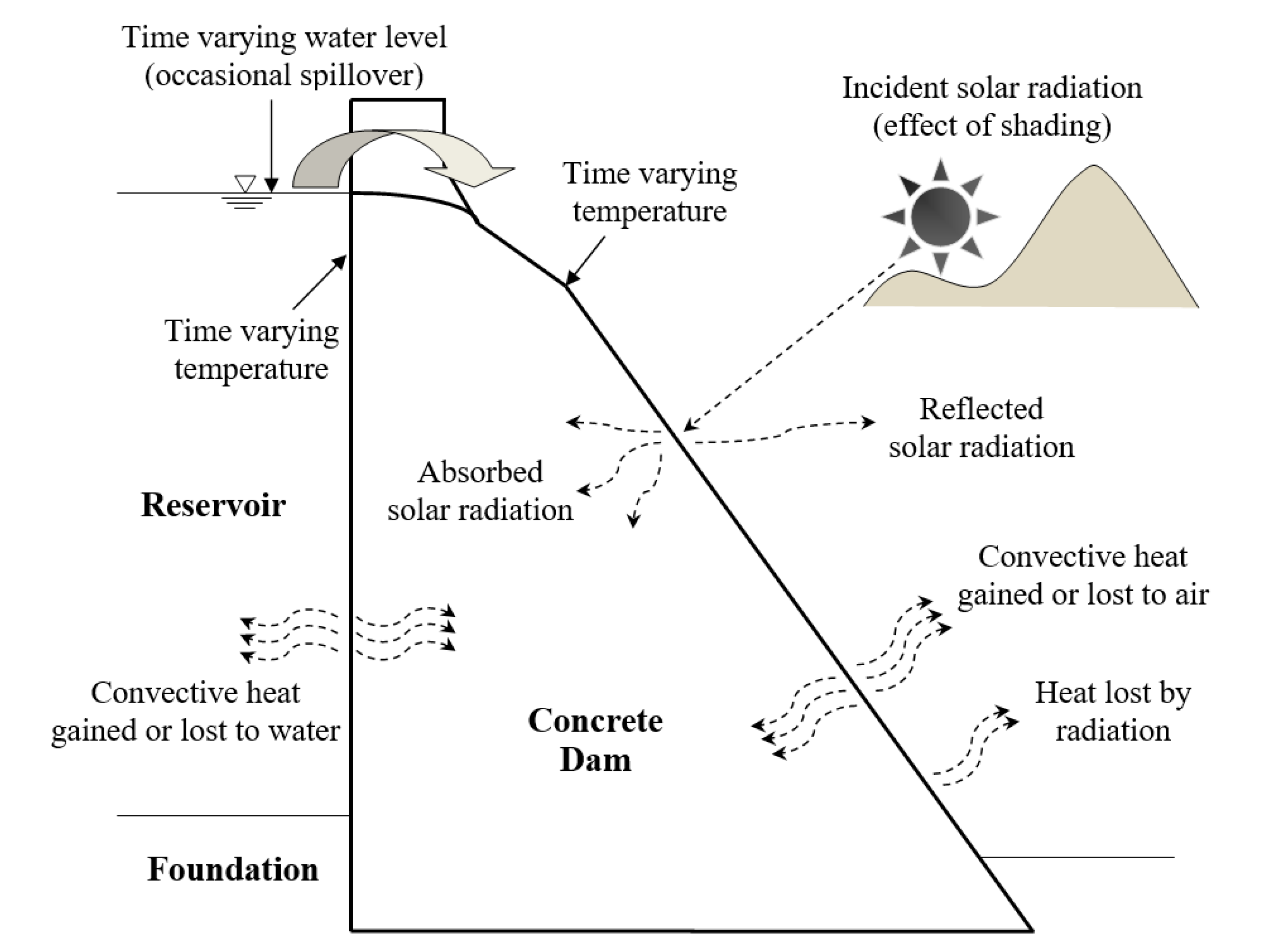
Figure 2.
The temperature monitoring system established in the central cross-section of the Moste Dam.
Figure 2.
The temperature monitoring system established in the central cross-section of the Moste Dam.
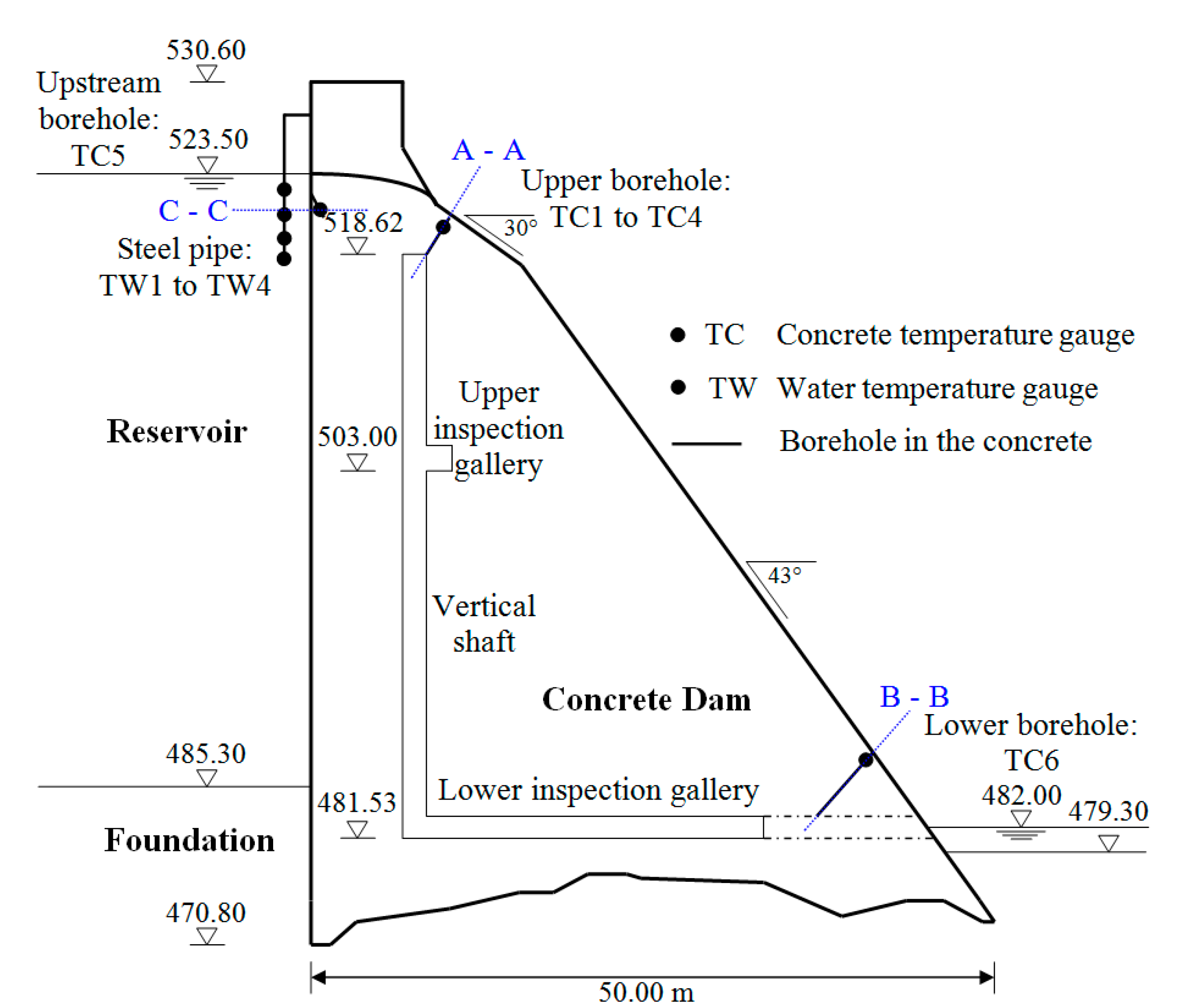
Figure 3.
The locations of the mobile automatic weather station (MAWS) and of the temperature gauges on the downstream side of the dam (Photo: P. Žvanut).
Figure 3.
The locations of the mobile automatic weather station (MAWS) and of the temperature gauges on the downstream side of the dam (Photo: P. Žvanut).
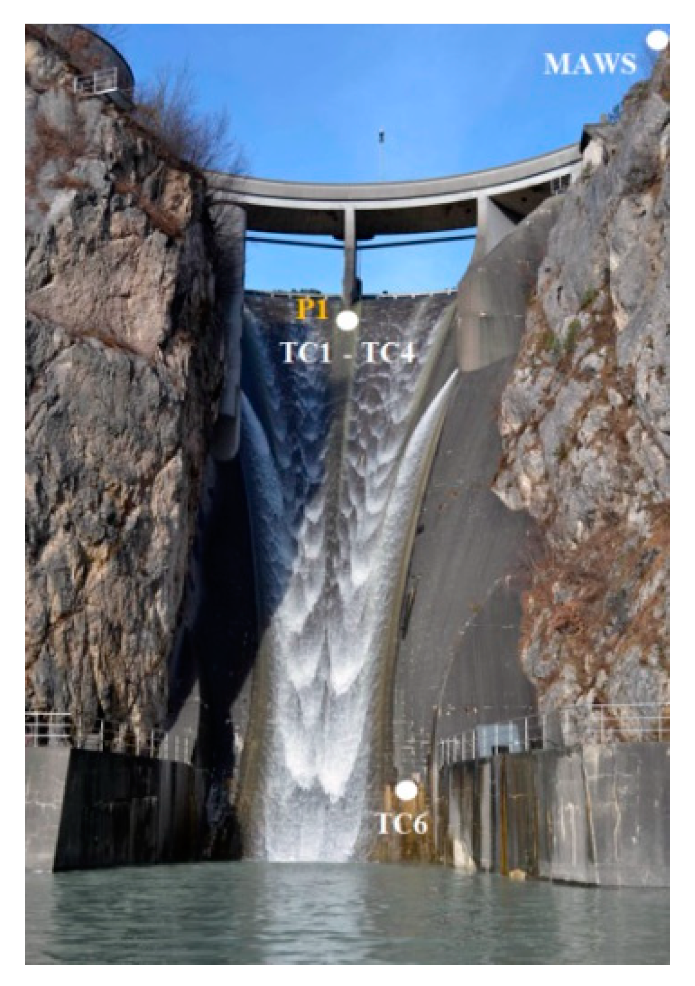
Figure 4.
The locations of the temperature gauges on the upstream side of the dam and in the protective pipe (Photo: P. Žvanut).
Figure 4.
The locations of the temperature gauges on the upstream side of the dam and in the protective pipe (Photo: P. Žvanut).
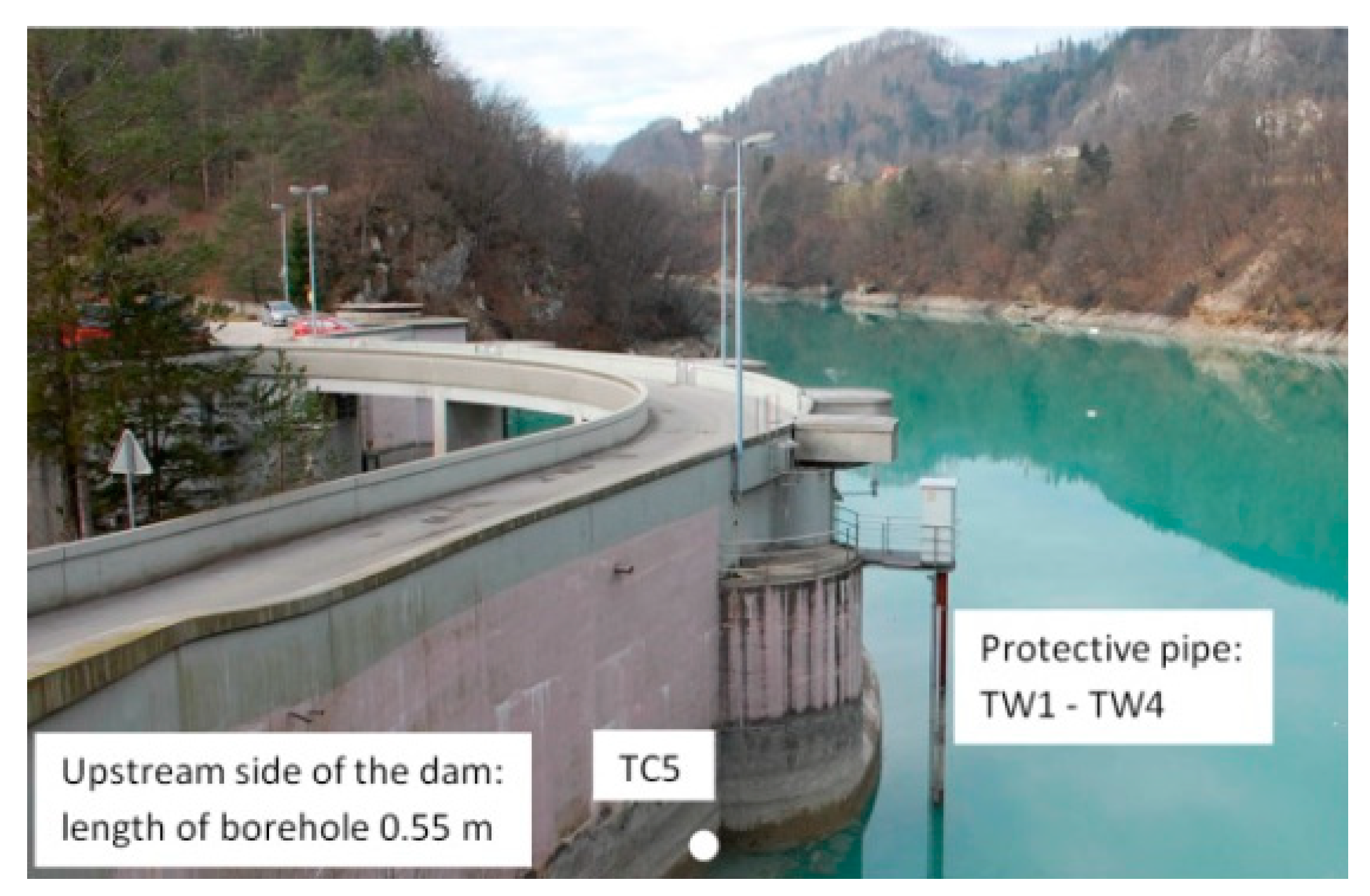
Figure 5.
The water level of the reservoir and the corresponding height of the spillover.
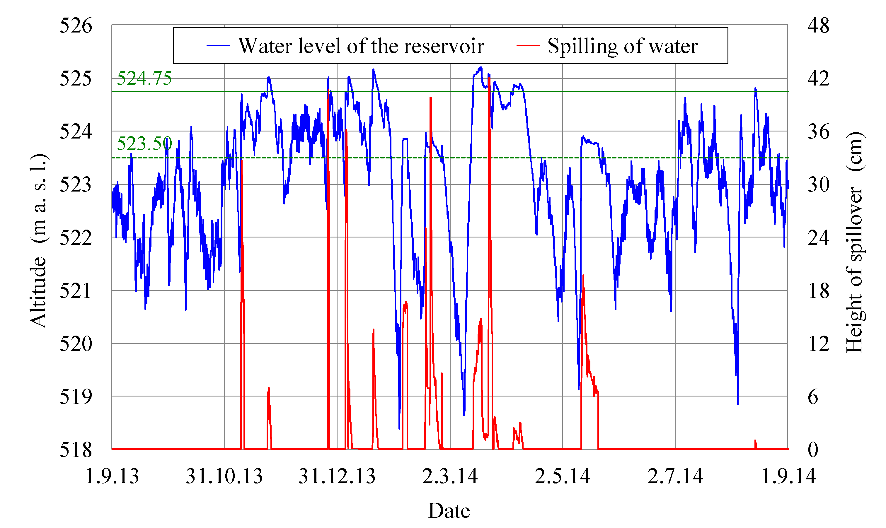
Figure 6.
The contour of the terrain as seen from point P1 and the virtual path of the Sun.
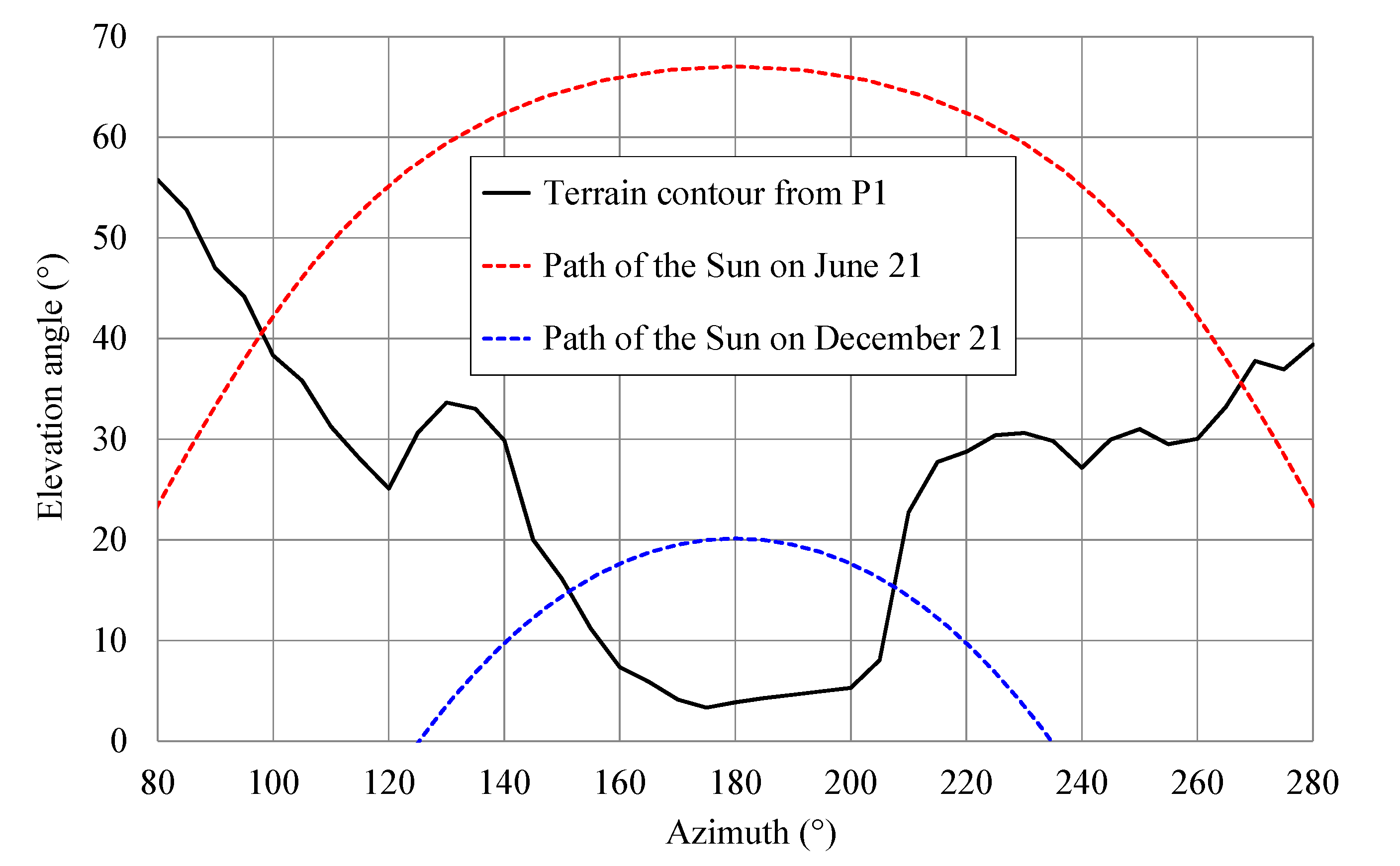
Figure 7.
The calculated absorbed heat flux due to theoretical year-round insolation and the measured absorbed heat flux at point P1.
Figure 7.
The calculated absorbed heat flux due to theoretical year-round insolation and the measured absorbed heat flux at point P1.
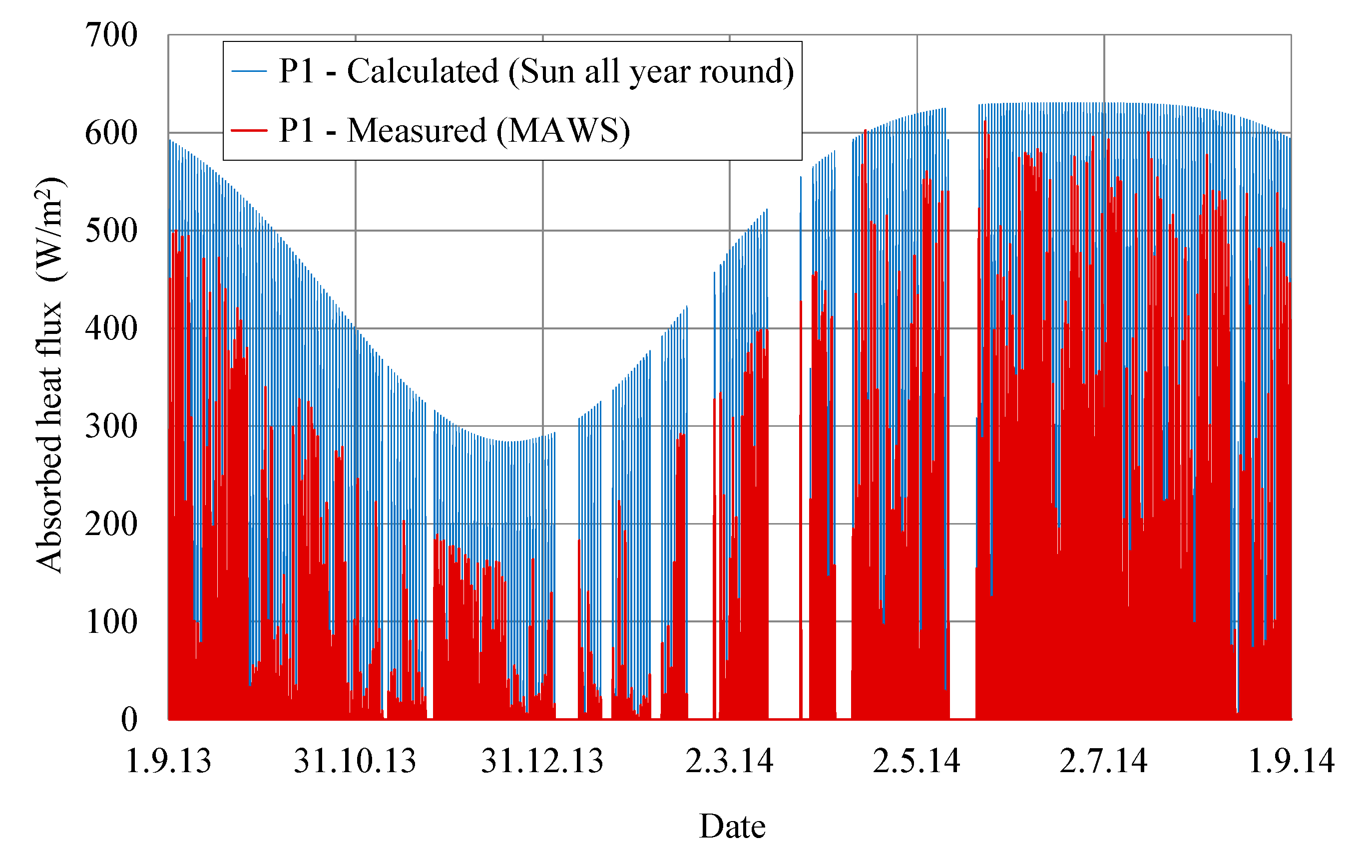
Figure 8.
The concrete temperatures at gauge TC1 during the analyzed 15-day period.
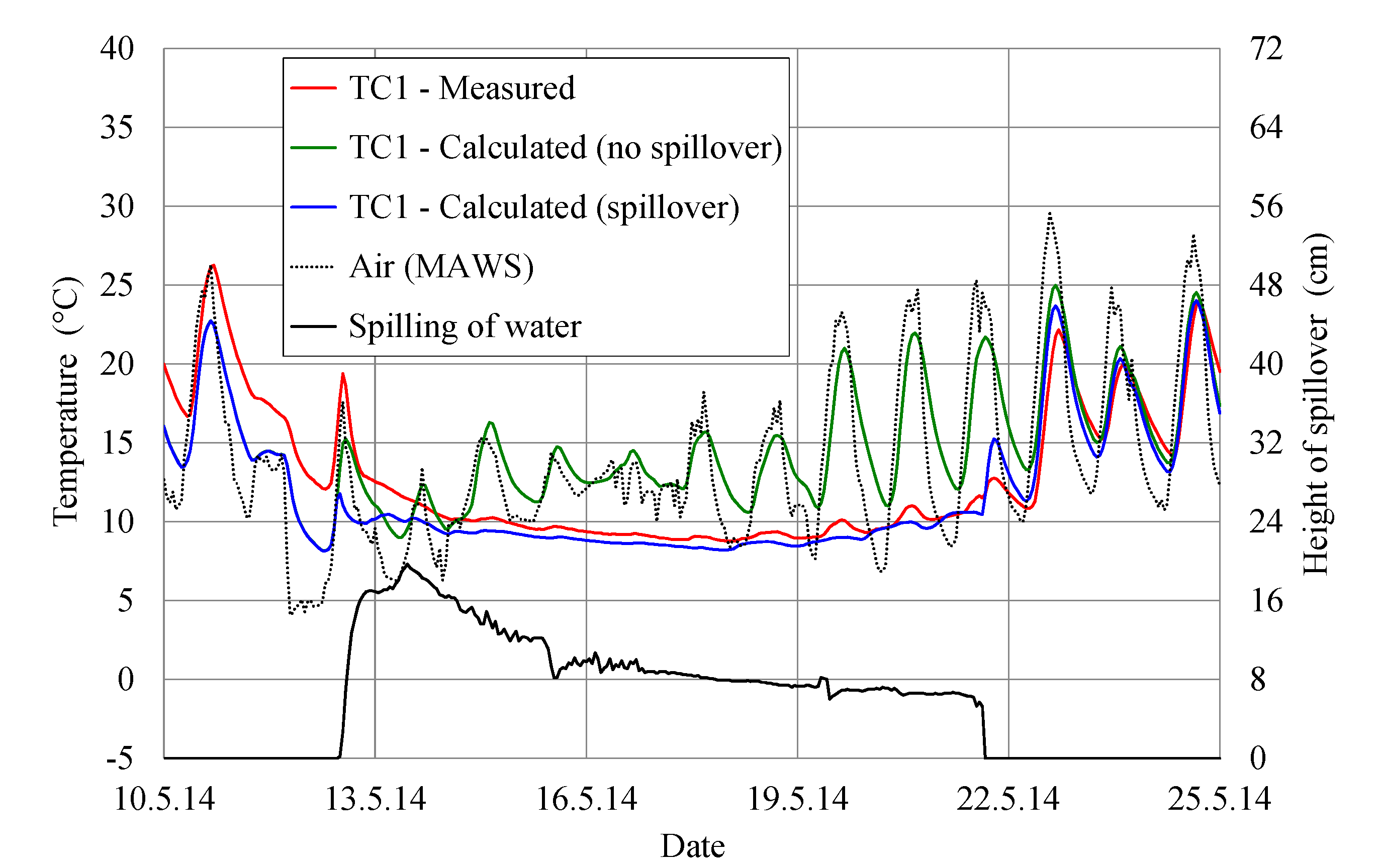
Figure 9.
The concrete temperatures at gauge TC4 during the analyzed 15-day period.
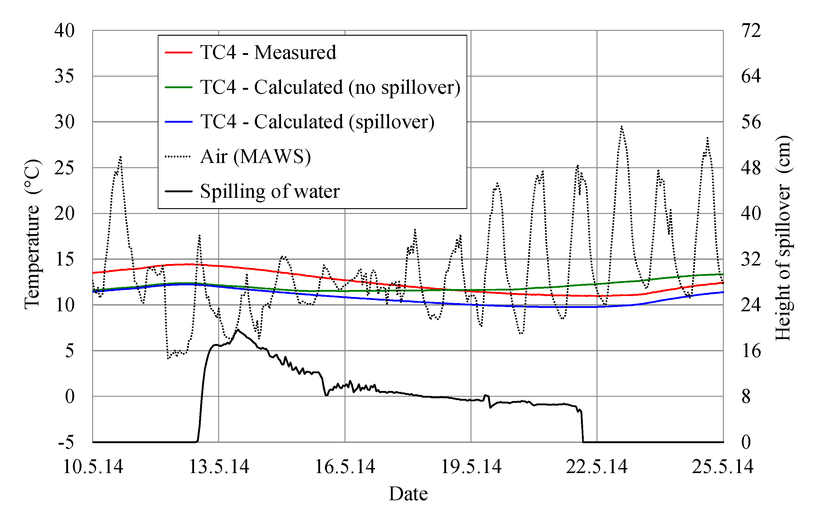
Figure 10.
The concrete temperatures at gauge TC5 during the analyzed 15-day period.
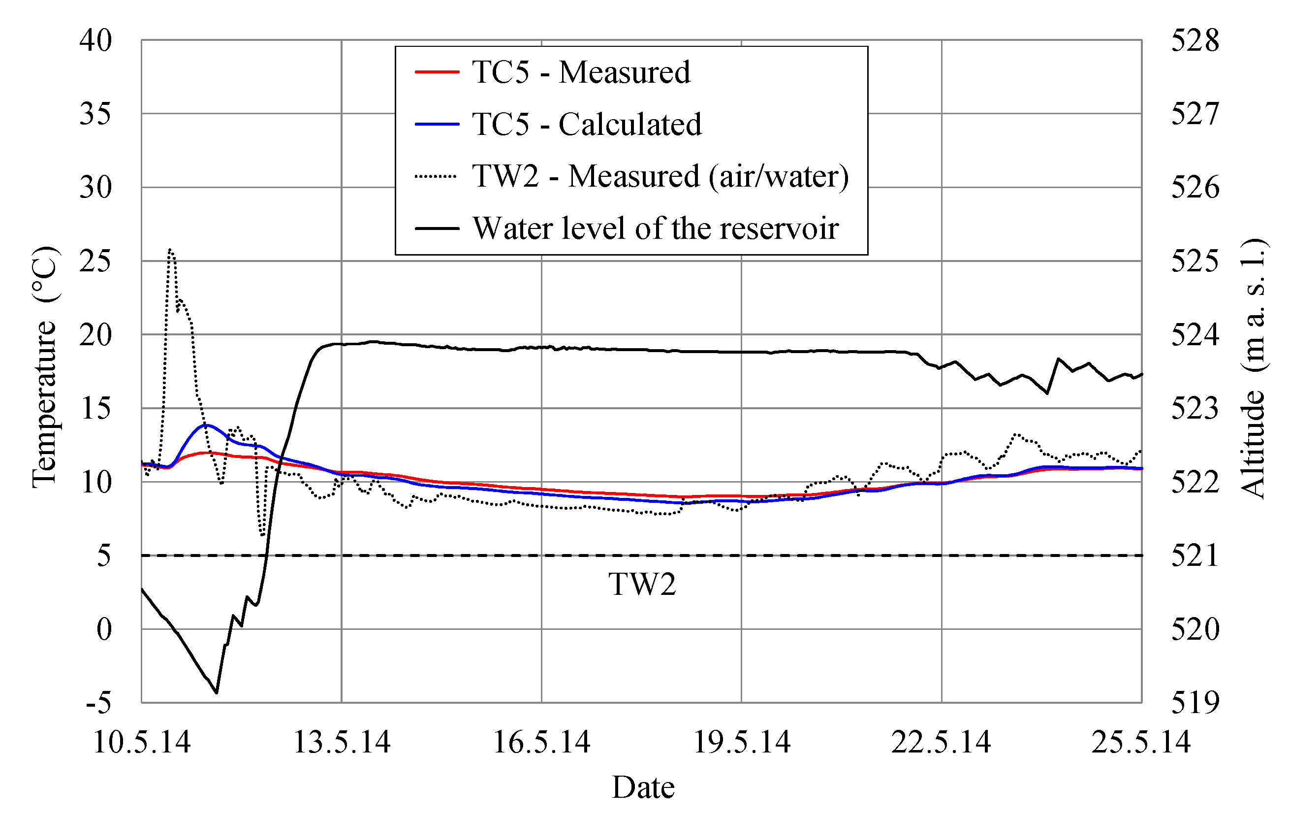
Figure 11.
The concrete temperatures at gauge TC6 during the analyzed 15-day period.
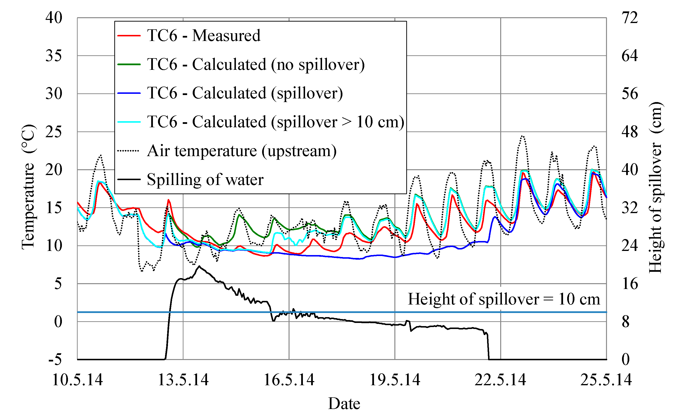
Figure 12.
The concrete temperatures at gauge TC3 during the analyzed year.
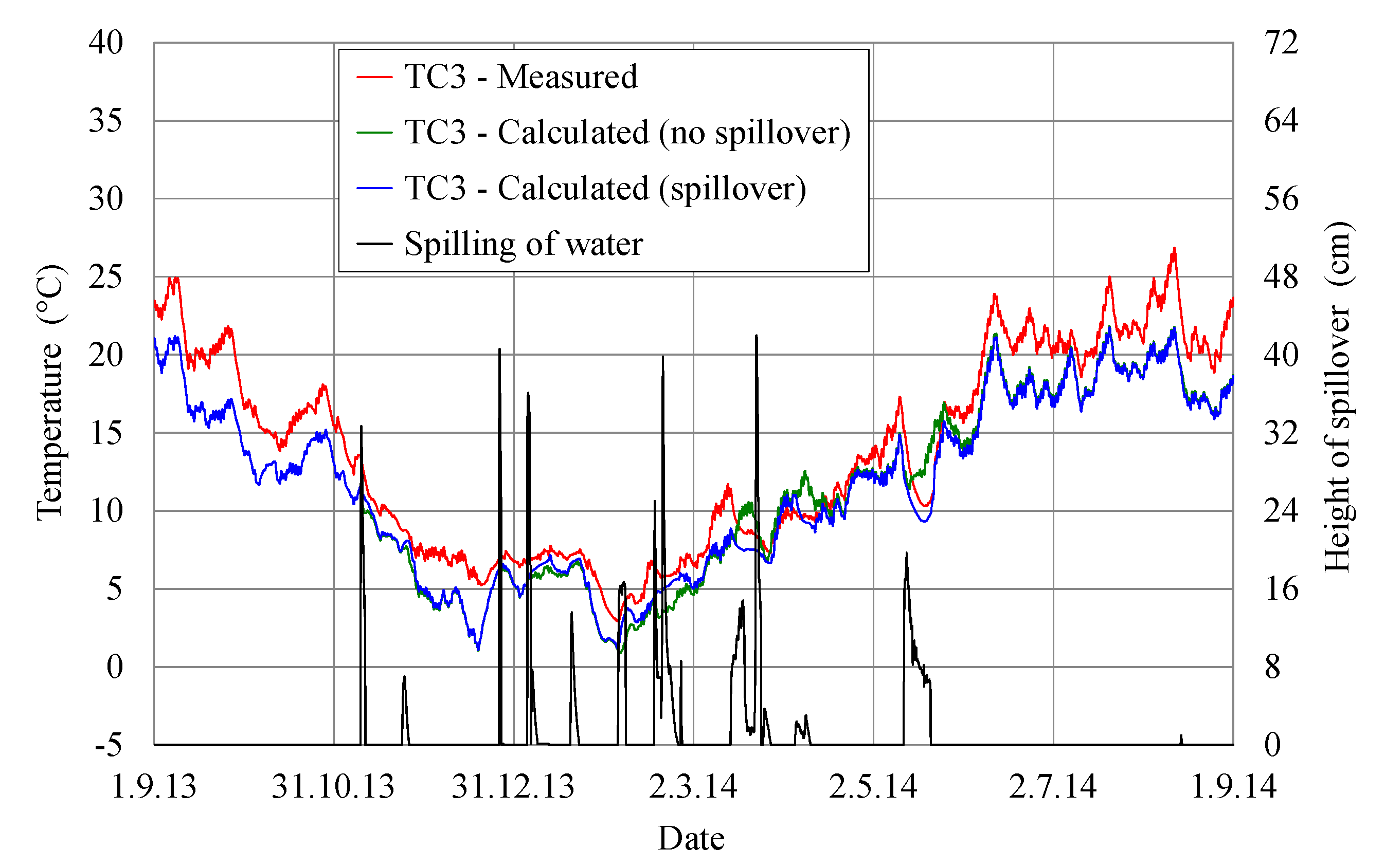
Figure 13.
The concrete temperatures at gauge TC4 during the analyzed year.
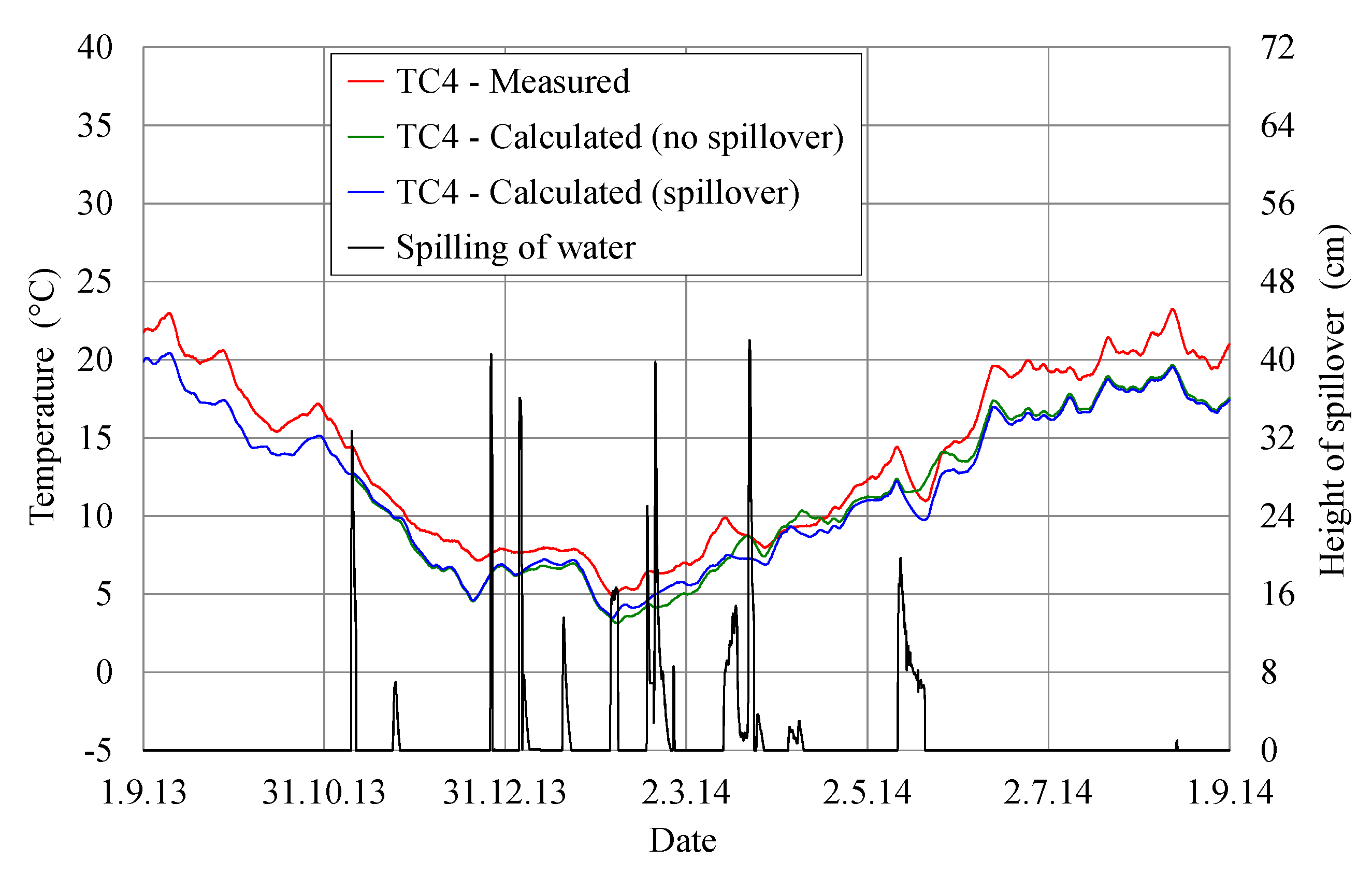
Figure 14.
The calculated temperature field of the Moste Dam (1 August 2014 at 12:00).
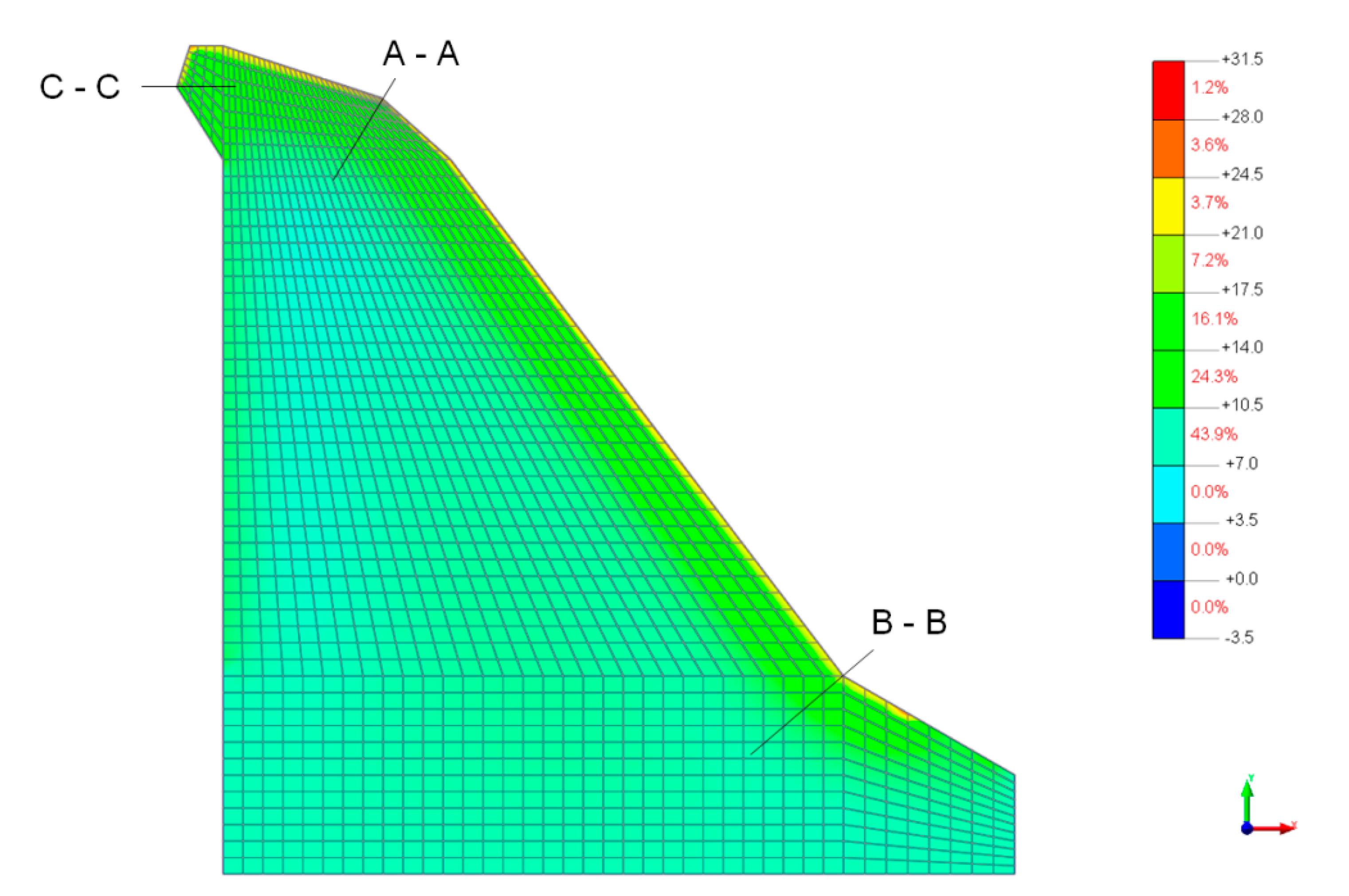
Figure 15.
The concrete temperatures at the two typical cross-sections in summer and in winter.
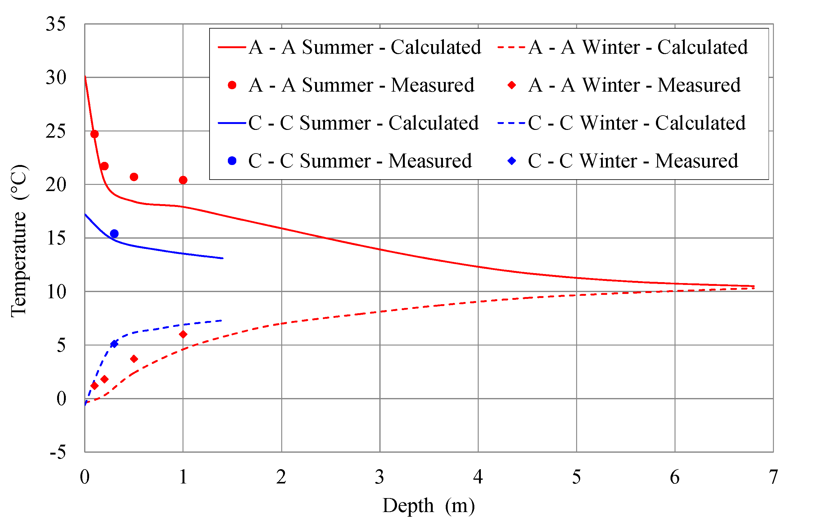
Figure 16.
Box-and-whiskers plots of the concrete temperatures at 12 selected points.

Table 1.
The thermal properties of the mass concrete.
| Material Property | Unit | Expected Value | Standard Deviation 1 |
|---|---|---|---|
| Density | kg/m3 | 2400 | 96 |
| Specific heat | J/(kg K) | 960 | 96 |
| Thermal conductivity | W/(m K) | 2.33 | 0.233 |
| Convection coefficient (air) | W/(m2 K) | 55.6 | 11.12 |
| Convection coefficient (water) | W/(m2 K) | 556 | 55.6 |
| Solar absorptivity | / | 0.65 | 0.0325 |
| Emissivity | / | 0.90 | / |
1 Taken into account in determining the uncertainty of the calculation results.
Table 2.
The temperature oscillations and time lags at gauges TC1 to TC4.
| Limit | Temperature (°C) | |||||||||
|---|---|---|---|---|---|---|---|---|---|---|
| Air | TC1 | TC2 | TC3 | TC4 | ||||||
| M 1 | M 1 | C 2 | M 1 | C 2 | M 1 | C 2 | M 1 | C 2 | ||
| Annual oscillations | T min | −9.5 | 0.9 | −4.6 | 1.4 | −2.4 | 2.9 | 1.1 | 4.9 | 3.5 |
| T max | 35.6 | 36.2 | 31.3 | 32.1 | 27.0 | 26.9 | 21.7 | 23.3 | 20.4 | |
| Diff. | 45.1 | 35.3 | 35.9 | 30.7 | 29.4 | 24.0 | 20.6 | 18.4 | 16.9 | |
| Time lag | T min | / | 3–4 3 | 4–5 3 | 10–12 3 | Several days | ||||
| T max | / | 1–2 3 | 2–3 3 | 10–12 3 | Several days | |||||
1 M: measured. 2 C: calculated. 3 Time lag in hours.
Table 3.
The temperature oscillations and time lags at gauge TC5.
| Limit | Temperature (°C) | |||||
|---|---|---|---|---|---|---|
| Air 1 | Water 1 | Water 2 | TC5 | |||
| M 3 | M 3 | M 3 | M 3 | C 4 | ||
| Annual oscillations | T min | −1.8 | 2.7 | 2.9 | 3.8 | 2.0 |
| T max | 32.1 | 19.0 | 16.6 | 17.6 | 18.8 | |
| Diff. | 33.9 | 16.3 | 13.7 | 13.8 | 16.8 | |
| Time lag | T min | / | / | / | 6–8 h | |
| T max | / | / | / | 5–6 h | ||
1 At gauge TW2 (i.e., 521 m a. s. l.). 2 At gauge TW1 (i.e., 519 m a. s. l.). 3 M: measured. 4 C: calculated.
Table 4.
The temperature oscillations and time lags at gauge TC6.
| Limit | Temperature (°C) | |||
|---|---|---|---|---|
| Air | TC6 | |||
| M 1 | M 1 | C 2 | ||
| Annual oscillations | T min | −5.8 | 1.0 | −1.9 |
| T max | 30.1 | 25.7 | 25.6 | |
| Diff. | 35.9 | 24.7 | 27.5 | |
| Time lag | T min | / | 3–4 h | |
| T max | / | 1–2 h | ||
1 M: measured. 2 C: calculated.
Table 5.
Locations of the 12 selected points at typical cross-sections.
| Point | Downstream–Above | Downstream–Below | Upstream | |||||||||
|---|---|---|---|---|---|---|---|---|---|---|---|---|
| A1 | A2 | A3 | A4 | A5 | B1 | B2 | B3 | B4 | B5 | C1 | C2 | |
| Depth (m) | 0.0 | 0.2 | 0.5 | 1.0 | 2.0 | 0.0 | 1.6 | 3.2 | 4.8 | 6.4 | 0.0 | 0.3 |
Table 6.
The calculated values of 7 statistics of the concrete temperatures at 12 selected points.
| Point | Temperature (°C) | |||||||
|---|---|---|---|---|---|---|---|---|
| n1 | X min4 | Q15 | Q25 | Q35 | X max4 | |||
| A1 | 60 | 30.24 | 1.15 | 28.1 | 29.20 | 30.25 | 31.03 | 32.6 |
| A2 | 60 | 20.34 | 0.37 | 19.6 | 20.10 | 20.30 | 20.60 | 21.1 |
| A3 | 60 | 18.48 | 0.22 | 18.1 | 18.30 | 18.50 | 18.60 | 18.9 |
| A4 | 60 | 18.00 | 0.17 | 17.7 | 17.90 | 18.00 | 18.10 | 18.3 |
| A5 | 60 | 15.95 | 0.19 | 15.5 | 15.80 | 15.95 | 16.10 | 16.3 |
| B1 | 60 | 23.28 | 0.60 | 22.0 | 22.90 | 23.30 | 23.70 | 24.7 |
| B2 | 60 | 15.93 | 0.14 | 15.6 | 15.80 | 15.90 | 16.00 | 16.2 |
| B3 | 60 | 12.79 | 0.17 | 12.5 | 12.68 | 12.80 | 12.90 | 13.2 |
| B4 | 60 | 11.13 | 0.13 | 10.9 | 11.00 | 11.10 | 11.20 | 11.5 |
| B5 | 60 | 10.40 | 0.08 | 10.3 | 10.30 | 10.40 | 10.40 | 10.6 |
| C1 | 60 | 17.21 | 0.08 | 17.1 | 17.20 | 17.20 | 17.23 | 17.4 |
| C2 | 60 | 14.82 | 0.08 | 14.7 | 14.80 | 14.80 | 14.90 | 15.0 |
1n: sample size. 2: sample mean. 3: standard deviation of the sample. 4X min, X max: minimum and maximum value of the sample elements. 5Q1, Q2, Q3: first, second and third quartile of the sample elements.
Publisher’s Note: MDPI stays neutral with regard to jurisdictional claims in published maps and institutional affiliations. |
© 2021 by the authors. Licensee MDPI, Basel, Switzerland. This article is an open access article distributed under the terms and conditions of the Creative Commons Attribution (CC BY) license (http://creativecommons.org/licenses/by/4.0/).
Share and Cite
MDPI and ACS Style
Žvanut, P.; Turk, G.; Kryžanowski, A. Thermal Analysis of a Concrete Dam Taking into Account Insolation, Shading, Water Level and Spillover. Appl. Sci. 2021, 11, 705. https://doi.org/10.3390/app11020705
AMA Style
Žvanut P, Turk G, Kryžanowski A. Thermal Analysis of a Concrete Dam Taking into Account Insolation, Shading, Water Level and Spillover. Applied Sciences. 2021; 11(2):705. https://doi.org/10.3390/app11020705
Chicago/Turabian StyleŽvanut, Pavel, Goran Turk, and Andrej Kryžanowski. 2021. "Thermal Analysis of a Concrete Dam Taking into Account Insolation, Shading, Water Level and Spillover" Applied Sciences 11, no. 2: 705. https://doi.org/10.3390/app11020705
Note that from the first issue of 2016, this journal uses article numbers instead of page numbers. See further details here.