Thermochemical Heat Storage in a Lab-Scale Indirectly Operated CaO/Ca(OH)₂ Reactor—Numerical Modeling and Model Validation through Inverse Parameter Estimation

Abstract

Calcium oxide/Calcium hydroxide can be utilized as a reaction system for thermochemical heat storage. It features a high storage capacity, is cheap, and does not involve major environmental concerns. Operationally, different fixed-bed reactor concepts can be distinguished; direct reactor are characterized by gas flow through the reactive bulk material, while in indirect reactors, the heat-carrying gas flow is separated from the bulk material. This study puts a focus on the indirectly operated fixed-bed reactor setup. The fluxes of the reaction fluid and the heat-carrying flow are decoupled in order to overcome limitations due to heat conduction in the reactive bulk material. The fixed bed represents a porous medium where Darcy-type flow conditions can be assumed. Here, a numerical model for such a reactor concept is presented, which has been implemented in the software DuMu${}^{\mathrm{x}}$. An attempt to calibrate and validate it with experimental results from the literature is discussed in detail. This allows for the identification of a deficient insulation of the experimental setup. Accordingly, heat-loss mechanisms are included in the model. However, it can be shown that heat losses alone are not sufficient to explain the experimental results. It is evident that another effect plays a role here. Using Bayesian inference, this effect is identified as the reaction rate decreasing with progressing conversion of reactive material. The calibrated model reveals that more heat is lost over the reactor surface than transported in the heat transfer channel, which causes a considerable speed-up of the discharge reaction. An observed deceleration of the reaction rate at progressed conversion is attributed to the presence of agglomerates of the bulk material in the fixed bed. This retardation is represented phenomenologically by mofifying the reaction kinetics. After the calibration, the model is validated with a second set of experimental results. To speed up the calculations for the calibration, the numerical model is replaced by a surrogate model based on Polynomial Chaos Expansion and Principal Component Analysis.

1. Introduction

Energy storage is regarded a key task for the transition from fossil to renewable sources of energy with fluctuating availability. With more than 50%, heat is the major part of end energy consumption [1]. To avoid losses of conversion from one type of energy to another (e.g., power to heat), energy is best stored in the form of its production or consumption. Within the different heat-storage options, namely sensible, latent and thermochemical, the latter is the most promising as it features high storage densities and the possiblity to store energy without losses. Different materials have been found to be suitable for thermochemical heat storage in material screenings [2,3,4]. Several material groups span a large range from low level to high temperature applications, therein carbonates [5], hydrates [6], oxides [7] and hydroxides. Within those, the group of hydroxides is environmentally friendly [8], cheap [9], and covers a wide range of reaction temperatures. Several applications are envisaged, such as domestic heating [10], enhancement of CHP plants [11] or concentrated solar-power plants [12]. So far, however, no technology is commercially available. Their development requires further research.

This work puts a focus on the reaction system CaO/Ca(OH)${}_2$ that is described by the following reaction equation:

$$Ca{O}_{\left(s\right)}+H_2{O}_{\left(g\right)}\rightleftharpoons Ca{\left(OH\right)}_{2,\left(s\right)}+\Delta H_R.$$

(1)

This reaction system has already been studied on different scales. Small-scale studies of a few grams of solid material addressed the cycling stability [13] and material parameters [8]. Furthermore, the reaction enthalpy and thermodynamic equilibrium was investigated. The reaction enthalpy lies within the range of $\Delta H_R=94.6\mathrm{kJ}/\mathrm{mol}$ [14] to $\Delta H_R=109\mathrm{kJ}/\mathrm{mol}$ [15]. For water vapor pressures between $1\times {10}^3$ to $3\times {10}^6$ Pa, applications between 550 K and 1000 K are feasible [8,14]. Studies on the reaction mechanisms deliver contradicting results: for example, Criado et al. [16] identified a shrinking core model, whereas Irabien et al. [17] found a pseudo-homogeneous model. Reference [18] assumes that the reaction kinetics depend strongly on the reaction conditions for pressure and temperature. This allows to conclude that the resulting reaction kinetics are thus subject to uncertainty. Nagel et al. [19] and Risthaus et al. [20] however state that at high pressure ranges, the reaction rate is only limited by heat transfer. They apply the reaction kinetics of Reference [21] which is based on theoretical considerations and does not obey a specific reaction mechanism. Michel et al. [22] presented another way of representing the reaction rate based on information about the propagation of the reaction front for a different reaction system. However, it is beyond the scope and aim of this study to introduce completely new reaction kinetics for the reaction system CaO/Ca(OH)${}_2$. Instead, we build upon the findings of Reference [20] and apply the reaction kinetics of Reference [21].

The reaction system CaO/Ca(OH)${}_2$ has been studied on larger scales in fixed-bed reactors. Schaube et al. [23] present a directly heated fixed-bed reactor at the laboratory scale, containing 60 g of reactive powder. Linder et al. [24] presented a reactor with an indirect heating concept on a kW-scale. Additionally, Criado et al. [16] and Angerer et al. [9] present concepts for fluidized bed reactors. To enhance the understanding of such laboratory experiments, they often come along with modeling [25]. Modeling is used for theoretical analysis, identification of mechanisms, and optimization.

For quantitatively reliable predictions, mathematical models need to be validated. While suitable experimental data for model validation is sparse and often subject to uncertainties, several models have been presented for fixed-bed thermochemical heat-storage reactors without proof of validation. Nagel et al. [26] study the influence of particle sizes, Nagel et al. [19] test different reaction kinetics, Ranjha et al. [27] address the heat-transfer enhancements by introducing fins, Seitz et al. [28] study the influence of porosity induced permeability alterations, and Balasubramanian et al. [29] investigate theoretically the performance of different suitable materials. Without validation, these models can only give qualitative insights.

Simulation results matching experimental data is a necessary, but not a sufficient condition for a validated model. If the experimental and the modeling data sets do not match, model parameters can be adjusted or additional terms can be introduced to represent further processes. Schaube et al. [30] adapted the reaction kinetics determined in Reference [8] in order to fit the modeling results to the experimental data of a directly heated fixed-bed reactor. For an indirectly heated reactor model, Linder et al. [24] and Risthaus et al. [20] introduce an additional, volume-based heat-loss term.

In this study, we present a numerical model that describes the indirectly heated reactor concept presented in Reference [31]. Our aim is to validate it based on the experimental data of References [20,31]. Risthaus et al. [20] present additional experimental and modeling results to the same setup at varying pressure conditions. However, the authors of the experiment detected unwanted heat losses across the reactor surface due to a defective insulation. In our opinion, the volumetric heat-loss terms introduced by Reference [20] to the same experimental setup lack physical substantiation and are rather a calibration term. With the present approach, we seek a match to the experimental data based on a more objective substantiation of the physical background. Bayesian parameter inference is used to find the location of the heat losses, given the experimental data for temperature at distinct locations and the overall conversion rate. The inverse modelling approach furthermore enables to study other uncertain parameters and mechanisms, such as heat transfer and the reaction rate. It corresponds to the model calibration. The model is validated subsequently with a different set of experimental data. We claim, that the second step is sufficient for model validation.

The numerical model and the simulation setup are presented in Section 2. Preliminary simulation results reveal, that the heat loss is not sufficient to represent the experimental data, but another process affects chemical reaction and heat transfer at progressed conversion. Using preliminary simulation results, we select in total seven parameters for calibration by inverse modeling in Section 3. Section 4 introduces the framework for Bayesian inference. In Section 5, we present and discuss the results of the model calibration. Subsequent model validation provides further proof of the model concept.

2. Numerical Model

The indirectly operated fixed-bed reactor concept consists of two functional units, the reactive bed where the reaction occurs, and the heat-transfer channel (HTF) that is placed in the reactive domain to transport the heat released or consumed by the chemical reaction. Only conductive heat but no mass is exchanged between the two units. Schmidt et al. [32] designed the reactor such that the resistance to heat transfer between the two domains is minimized. Below, we introduce the experimental reactor setup and simplifying assumptions for the numerical model, which is presented thereafter.

2.1. Experimental Setup

Figure 1 left shows the reactor setup of Reference [32]. The fixed bed contains a volume of 4.8 L solid material. It is placed between filter plates which represent the connection to the surrounding vapor vessel. There, water vapor, the reaction fluid, is provided with a constant gas pressure. Consumption or production of water vapor by the chemical reaction in the reactive bed induces an advective flux between the reactive bed and the vapor vessel. A HTF channel is placed in the middle of the reactive bed and separates it into two parts. Air is used as heat-transfer fluid in the HTF channel. The reactor stretches 150 mm in the z-direction (third dimension).

The reactive bed is initially filled with CaO-powder. The discharge reaction is initiated by increasing the pressure in the vapor vessel. CaO powder starts to convert to Ca(OH)${}_2$ by consuming water vapor. The released heat is conducted towards the HTF channel. Here, a constant volume flux of air removes the heat and keeps the reaction going until complete conversion. The vapor pressure in the vessel and the volume flux of air determine the temperature level of the reaction and the speed of discharge. In order to monitor the reaction, thermocouples at several locations indicated in Figure 1 monitor the temperature. Furthermore, the global conversion is measured as a function of the consumed water [32]. Experimental results for two different experimental runs, namely Case A in Reference [31] and a reference case in Reference [20], will serve for model calibration and subsequent validation. For details concerning the operation procedure we refer to References [31,32].

The vessel containing all the reactor units is insulated. The casing is furthermore heated to the same temperature as imposed in the HTF channel. Nevertheless, temperatures measured by the thermocouples fall below the predefined temperature of the HTF channel after conversion: 764 K at measurement point T1, 763–765 K at measurement point T3 and 757 K at measurement point T7 [31]. The temperature in the HTF channel before entering the reactive bed is constant. This is confirmed by measurements, see Reference [32]. Thus, the heat must be lost due to a lower temperature in the vapor vessel. However, there are no temperature measurements available and thus, the location and the amount of the heat losses are unknown.

2.2. Model Setup

Different physical processes dominate in the two functional units, the reactive bed and the heat transfer channel. Thus, we split the reactor into two separate domains, (i) the free flow channel (HTF channel) with the air flux and (ii) the porous-medium domain with the reactive bulk and internal water-vapor fluxes. Both domains are coupled by conductive heat flow. Due to symmetry, the reaction domain is reduced to the reaction bed above the heat transfer channel according to Reference [20]. The simulation setup is displayed in Figure 1 on the top right. The boundary effects of the third dimension are assumed to be negligibly small, so that the numerical model represents the experiment in two dimensions. The numerical model is based on the following simplifying assumptions:

• The air density in the HTF channel is a function of temperature only (the influence of pressure variation on the density is negligible).
• Gas flow in the HTF channel is laminar with a fully developed viscous boundary layer.
• Heat conduction in the metal casing is much larger than in the HTF channel and the porous bulk. The casing is thus not considered in the model.
• There is local thermal equilibrium in the reactive bulk.
• Gas flow in the reactive bulk is creeping.

The following sections contain the description of the two subdomain models, their coupling and the description of the heat losses.

2.2.1. Sub-Model of the Reactive-Bed Domain

The reactive bulk of solid particles is assumed as a porous medium at the the scale of a representative elementary volume (REV) [33,34]. Balance equations are formulated for each chemical component, that is, CaO, Ca(OH)${}_2$ and H${}_2$O in terms of molar fractions for water, and volume fractions for the solid components, respectively. By balancing both solid components separately, the model is able to represent the change in solid volume and, thus, in porosity due to the chemical reaction. This is in contrast to the model described in Reference [20], where the solid volume is constant. The importance of taking the solid-volume change into account is described in detail in Reference [28] for a directly heated fixed-bed reactor. The chemical reaction is included by reaction kinetics as source/sink terms.

The gaseous component is transported via advection due to pressure gradients. The mass balance equation of the gaseous component considers changes in the gas storage due to changes in density, advection, and sources/sinks:

$$\frac{\partial \left({\varrho }_g{\varphi }_g\right)}{\partial t}-\nabla ·\left({\varrho }_g\mathbf{v}\right)=(1-{\varphi }_g)·\frac{dX}{dt},$$

(2)

with gas density ${\varrho }_g$, porosity ${\varphi }_g$, velocity $\mathbf{v}$ and reaction rate $\frac{dX}{dt}$. The factor $(1-{\varphi }_g)$ takes into account that the reaction occurs only in the solid volume fraction. The gas velocity $\mathbf{v}$ is determined by Darcy’s law:

$$\mathbf{v}=\frac{\mathbf{K}}{{\mu }_g}\left(\mathrm{grad}p\right),$$

(3)

with the permeability $\mathbf{K}$, the gas viscosity ${\mu }_g$, and pressure p.

The solid bulk is considered as rigid. Thus, the solid mass balance equations contain only terms for storage and reaction, but no advection term:

$$\frac{\partial \left({\varrho }_{\lambda }{\varphi }_{\lambda }\right)}{\partial t}=\pm (1-{\varphi }_g)·\frac{dX}{dt},\lambda \in \{\mathrm{CaO},\mathrm{Ca}{\left(\mathrm{OH}\right)}_2\},$$

(4)

with the solid volume fractions ${\varphi }_{\lambda }$. Due to stoichiometry, the amount of reaction rate $\frac{dX}{dt}$ is the same for CaO and Ca(OH)${}_2$ but with different signs.

The bulk energy balance equation considers heat flux by gas advection and heat conduction in the porous bulk. Alterations in pressure, temperature, and presence of phases change the energy stored in the system. The chemical reaction releases/consumes reaction enthalpy $\Delta h_R$. Assuming local thermal equilibrium, see also Reference [35], the energy balance equation is written as:

$$\begin{array}{c}\hfill \frac{\partial }{\partial t}\left({\varphi }_g{\varrho }_g{u}_g\right)+(1-{\varphi }_g){\varrho }_s{c}_{ps}\frac{\partial T}{\partial t}+\nabla ·\left({\varrho }_g\mathbf{v}{h}_g\right)-\nabla ·({\lambda }_{eff}\nabla T)=\\ \hfill (1-{\varphi }_g)·\frac{dX}{dt}\left(\Delta h_R-\frac{{\varphi }_g}{1-{\varphi }_g}\frac{p}{{\varrho }_g}\right),\end{array}$$

(5)

with the specific internal energy of the gas $u_g$, the solid heat capacity $c_{ps}$, the specific enthalpy of the gas $h_g$, and the effective heat conductivity ${\lambda }_{eff}$. $c_{ps}$ is calculated by volume averaging over the present solid phases, ${\lambda }_{eff}$ by volume averaging over all phases. The energy source term due to reaction is reduced by the volume expansion ($p/{\varrho }_g$) to take the phase change of the gaseous component in the chemical reaction into account.

To determine the reaction rate, we build upon the reaction kinetics referred to as “Fast” by Reference [20] or “Simple” by Reference [19]. The reaction rate is obtained based on the conditions of temperature, water vapor pressure, and the degree of conversion. This is based on theoretical considerations by Reference [21] and has been used in several studies [19,20,26]. The authors of References [19,20] state that for sufficiently high vapor pressures, this reaction is sufficiently accurate. However, we introduce here an additional term, that reduces the reaction rate for progressed conversion $(1-X)$ with X the conversion. This term and its exponent $k_{R,2}$ will be subject to optimization and is addressed in more detail in Section 3.

$$\frac{dX}{dt}=k_{R,1}{(1-X)}^{1+k_{R,2}}\frac{T-T_{eq}}{T_{eq}}({\varrho }_{\mathrm{CaO}}-{\varrho }_{\mathrm{Ca}\left(\mathrm{OH}\right){}_2}),$$

(6)

with rate constants $k_{R,1}$, and $k_{R,2}$, the conversion $X={\varphi }_{\mathrm{Ca}\left(\mathrm{OH}\right){}_2}/{\varphi }_{\mathrm{Ca}\left(\mathrm{OH}\right){{}_2}_{max}}$. The equilibrium temperature $T_{eq}$ is determined by the van’t Hoff equation. We use here the formulation retrieved by Reference [14], as this matches the equilibrium temperature best for the studied pressure range:

$$\ln \left(\frac{p_{H_{2}O}}{1\mathrm{bar}}\right)=\frac{11375\mathrm{K}}{T_{eq}}+14.574.$$

(7)

2.2.2. Formulation of the Heat Loss

As outlined earlier, a temperature difference between the outer reactive-bed boundary and the vapor vessel is considered to cause the heat losses in the experiments of Reference [32]. It is assumed that the heat is transported between the two parallel plates (i.e., the filter plate and the vapor vessel casing, see Figure 1, left) with water vapor between them. The height of the reactive bed (2 cm) is much smaller than the length (1.6 m), so that we neglect heat losses on its vertical boundaries. According to Reference [36], several heat-transport mechanisms overlap and need to be considered: free convection, radiation, and heat conduction. The different heat-transport mechanisms share the same driving force, namely the difference in the temperature of the bounding walls of the reactive bed and the vapor vessel. For radiation, however, the driving force is proportional to the difference in temperatures raised to the power of four. Representing all mechanisms independently would produce several new parameters, all of which bear uncertainty. Additionally, the exact dimensions of the vapor vessel are not indicated in Reference [32]. We aim at determining the overall heat loss in a spatially resolved manner, regardless of which mechanism dominates. Thus, for simplicity, we choose the following form for the overall heat-loss flux:

$$q_{e,loss}=(T(y=y_{max})-T_{BC}){\alpha }_{loss},$$

(8)

with the heat-loss coefficient ${\alpha }_{loss}$, the temperature in the reactive bulk at the top boundary (at location $y=y_{max}$), and the temperature of the pressure-vessel casing $T_{BC}$. As the temperatures measured at the locations T1, T3 and T7 all are different, we assign three degrees of freedom to the temperature distribution:

$$T_{BC}=k_1{x}^2+k_{2}x+k_3.$$

(9)

The constants $k_1$ to $k_3$ and the heat-loss coefficient ${\alpha }_{loss}$ are calibration parameters in the inverse modeling. The loss term is assigned to the degrees of freedom at the upper boundary of the porous bulk simulation domain.

2.2.3. Model of the Heat-Transfer Channel

Whereas the porous domain is represented in 2D to depict the spatial temperature profile, we reduce the flow in the HTF channel to 1D on the basis of the flow profile of a plate flow. Due to the small height of the HTF channel (1 mm) and a moderate mass flux, the Reynolds-numbers (Re) range between 900–1000. This indicates that the flow is laminar and far away from the transition to turbulent flow at Re ≈ 2200 [37]. According to Reference [38], compressiblity effects are only relevant for large velocities (i.e., for Mach number larger than 0.3) and are thus neglected. Thus, the Hagen-Poiseuille law describes the momentum balance of the channel flow. The combined mass and momentum balance equation results to:

$$\frac{\partial {\varrho }_g}{\partial t}-\nabla ·\left({\varrho }_g\frac{K}{{\mu }_g}\mathrm{grad}p\right)=0,$$

(10)

with the permeability K for plate flow and the channel thickness d, $K=\frac{1}{12}{d}^2$ according to the Hagen-Poiseuille law. The energy balance of the HTF channel contains the same terms as Equation (5) reduced by the contributions of the solid phases:

$$\frac{\partial }{\partial t}\left({\varrho }_g{u}_g\right)+\nabla ·\left({\varrho }_g\left(\frac{K}{{\mu }_g}\mathrm{grad}p\right)h_g\right)-\nabla ·({\lambda }_g\nabla T)=2·q_e.$$

(11)

The heat exchange between reactive bulk and HTF channel is included by the source term $q_e$, here multiplied with 2 since only half the reaction bulk domain but the complete HTF channel are resolved. The coupling term $q_e$ is addressed in the following section.

2.2.4. Coupling of the Two Domains

It is assumed that there is no temperature jump between the porous-medium side of the metal plate and the free-flow side, that is, the influence of the metal plate between the bulk domain and the HTF channel is neglected. At the interface between the two domains, the heat fluxes sum up to zero:

$$q_{e,HTF}=q_{e,bulk}=q_e.$$

(12)

The heat flux in the porous bulk is purely convective:

$$q_{e,bulk}={\lambda }_{eff}\frac{T_W-T_{bulk,y=\Delta y/2}}{\Delta y/2},$$

(13)

with the wall temperature $T_W$ at the interface, the temperature in the bulk grid cell closest to the HTF channel $T_{bulk}$, and the hight of the bulk grid cell y.

In the free flow, forced convection determines the heat flow:

$$q_{e,HTF}={\alpha }_{HTF}(T_{HTF}-T_W),$$

(14)

with $T_{HTF}$ the temperature in the middle of the HTF channel. The heat-transfer coefficient ${\alpha }_{HTF}$ is crucial for correct representation of the heat flux. It depends on the fluid properties, which change with pressure and temperature; however, it is common to assume ${\alpha }_{HTF}$ as constant over the given surface [39]. It is estimated based on the Nusselt number Nu $=\frac{\alpha D}{{\lambda }_g}$, with D, the hydraulic diameter. Reference [36] lists the value Nu = 8 for a flat-plate cross section with a fully developped boundary layer and laminar flow. With the gas properties of air at 773 K [40] and the thickness of the HTF channel, the heat-transfer coefficient is in the range of ${\alpha }_{HTF}=440[\mathrm{W}/{\mathrm{m}}^2\mathrm{K}]$. Reference [20] follows the instructions of Reference [37] and yield ${\alpha }_{HTF}=250[\mathrm{W}/{\mathrm{m}}^2\mathrm{K}]$ for heat transfer between the steel casing to the heat-transfer flux. As a correct value of ${\alpha }_{HTF}$ is important to determine the heat flux between reactive bulk and HTF channel correctly, this parameter will also be calibrated by inverse modeling.

The two Equations (13) and (14) allow for eliminating the unknown temperature at the wall $T_w$. The coupling heat flux is then only a function of the known temperatures $T_{HTF}$ and $T_{bulk}$. The locations of the unknown variables are indicated in Figure 1 on the bottom right.

2.2.5. Software Framework of the Numerical Model

The model ist implemented in the open-source software ${\mathrm{DuMu}}^{\mathrm{x}}$ [41]. The simulation domain is spatially discretized with cell-centered finite volumes. The model results have been tested for grid convergence. For time discretization, the implicit Euler method is used. The coupling between the two adjacent domains is described in detail in Reference [41]. Both domains including all balance equations are solved monolithically.

2.3. Simulation Setup

The boundary conditions are listed in

Table 1. Boundary and initial conditions with: $q_{air}$ source term for the component air, $q_{\mathrm{H}{}_2\mathrm{O}}$ water source term, $q_{\mathrm{Ca}\left(\mathrm{OH}\right){}_2}$ Ca(OH)${}_2$  source term, $q_{\mathrm{CaO}}$ CaO source term, $q_e$ energy source term. The initial temperature for all simulation cases is $T_{init}=773\left[\mathrm{K}\right]$.

Domain	Location	PriVar and Value
HTF channel	$t=0$	$p=p_{HTF,init}$, $T=T_{init}$
	$x=0$	$q_{air}=q_{air}$; $T=T_{init}$
	$x=x_{max}$	$p=p_{HTF,init}$; $q_{energy}=2q_e$
Porous Bulk	$t=0$	$p_{\mathrm{H}{}_2\mathrm{O}}=p_{bulk,init}$; $T=T_{init}$; ${\varphi }_{\mathrm{CaO}}=0.1113[-]$, ${\varphi }_{\mathrm{Ca}\left(\mathrm{OH}\right){}_2}=0.0[-]$
	$y=0$	$q_{\mathrm{H}{}_2\mathrm{O}}=0$; $q_{\mathrm{CaO}}=q_{\mathrm{CaH}}=0$
		$q_{energy}=q_e$
	$y=y_{max}$	$p_{\mathrm{H}{}_2\mathrm{O}}=p_{bulk,init}$; $q_{\mathrm{CaO}}=q_{\mathrm{CaH}}=0$;
		$q_{energy}=\frac{{\rho }_{\mathrm{H}{}_2\mathrm{O}}{K}_{bulk}}{{\mu }_{\mathrm{H}{}_2\mathrm{O}}}\nabla p_{y=y_{max}}·h(\mathrm{H}{}_2\mathrm{O},T_{y=y_{max}})+(T(y=y_{max})-T_{BC}){\alpha }_{loss}$
	$x=0$ & $x=z$	$q_{\mathrm{H}{}_2\mathrm{O}}=q_{\mathrm{CaO}}=q_{\mathrm{CaH}}=0$; $q_{energy}=(T\left(xy\right)-T_{BC}){\alpha }_{loss}$

.

Table 2. Material parameters.

Property	Symbol	Value
Reference porosity (according to Reference [20])	${\varphi }_{\mathrm{g}}$	0.773
Density Ca(OH)${}_2$ [26]	${\varrho }_{\mathrm{Ca}}{\left(\mathrm{OH}\right)}_2$	2200 kg m${}^{-3}$
Density CaO [42]	${\varrho }_{\mathrm{CaO}}$	3340 kg m${}^{-3}$
Permeability (according to Reference [20])	$\mathbf{K}$	8.8 × 10${}^{-12}$ m${}^2$
Specific heat capacity Ca(OH)${}_2$ [26]	$c_{\mathrm{p}\mathrm{Ca}{\left(\mathrm{OH}\right)}_2}$	1530 J kg${}^{-1}$ K${}^{-1}$
Specific heat capacity CaO [26]	$c_{\mathrm{p}\mathrm{CaO}}$	934 J kg${}^{-1}$ K${}^{-1}$
Solid heat conductivity [8]	${\lambda }_{\mathrm{s}}$	0.4 W m${}^{-1}$K${}^{-1}$
Reaction enthalpy [8]	$\Delta h_{\mathrm{R}}$	104.4 kJ mol${}^{-1}$

contains specific material parameters. The values for the vapor pressure and the air volume flux are specific to the two experimental scenarios for calibration (Case S17) and validation (Case R20). These values are given in

Table 3. Experimental setups, as basis for the simulations.

Case	Vapor Pressure ${\mathit{p}}_{\mathit{bulk},\mathit{init}}$ [kPa]	Air Flux ${\mathit{q}}_{\mathit{air}}$ $\left[\frac{\mathbf{kg}}{\mathbf{h}}\right]$
Case 17 (according to case A in Reference [31])	470	16
Case 20 (according to reference case in Reference [20])	270	25

.

3. Preliminary Calibration Attempt and Selection of Parameters for Optimization

We ran preliminary simulations in the attempt to calibrate, and, eventually, validate the model based on expert knowledge and trial-and-error changes of parameters. This did not lead to satisfactory results, but we can use this preliminary attempt for selecting the parameters related to heat transfer, heat loss, and heat release that are later on used in the optimization procedure, and we also define their ranges. These simulations are based on the experimental setup representing Case S17, see Table 3. Results with a linear $T_{BC}$ distribution (i.e., $k_1=0$, $k_2=-5.567$, and $k_3=764.99$) and the heat transfer parameters ${\alpha }_{HTF}=275$ $\mathrm{W}/{\mathrm{m}}^2\mathrm{K}$ and ${\alpha }_{loss}=30$ $\mathrm{W}/{\mathrm{m}}^2\mathrm{K}$ are shown in Figure 2 in orange. The simulated curves for the three temperatures T1, T3, and T7 roughly match the arrival time of the temperature jump after conversion in the respective region. However, the temporal temperature distribution differs between experiment and simulation. The slope at the temperature jump is much steeper in the simulation than in the experiment.

This indicates that further processes occur at progressed conversion and overlap the release of heat due to the reaction, additionally to the heat loss and transport in the reactive bed. In order to identify those processes, we tested the influence of a variation in the following parameters on the simulation results: a porosity induced permeability alteration, the solid heat conductivity and the constants of the reaction kinetics. The changed parameters for each simulation are listed in

Table 4. Summary of the simulation cases displayed in Figure 2. The units of the parameters are listed in Table 5.

Case	${\mathit{\alpha }}_{\mathit{HTF}}$	${\mathit{\alpha }}_{\mathit{loss}}$	K	${\mathit{\lambda }}_{\mathbf{CaO}}$	${\mathit{\lambda }}_{\mathbf{Ca}\left(\mathbf{OH}\right){}_2}$	${\mathit{k}}_{\mathit{R},1}$	${\mathit{k}}_{\mathit{R},2}$
Heat losses	275	30	$8.8\times {10}^{-12}$	0.4	0.4	10	0
Permeability	275	30	$8.8\times {10}^{-12}$	0.4	0.4	10	0
			$8.8\times {10}^{-11}$
Heat conductivity	275	30	$8.8\times {10}^{-12}$	0.3	0.5	10	0
Reaction param 1	275	30	$8.8\times {10}^{-12}$	0.4	0.4	0.2	0
Reaction param 2	275	30	$8.8\times {10}^{-12}$	0.4	0.4	10	2

. Figure 2 displays the simulation results.

3.1. Porosity Induced Permeability Change

Within the reactive bed of the indirectly operated reactor, most of the heat of reaction is transported due to heat conduction. The pressure gradients in the reactive bed are small and hence the advective heat transport. During the reaction, the solid volume and, thus, the permeability change. This has a notable effect on directly operated reactors [28] and tests confirmed that this also affects the heat transport in the indirectly operated reactor type. The gray dashed line in Figure 2 shows a simulation with permeability change from $8.8\times {10}^{-12}$ m${}^2$ to $8.8\times {10}^{-11}$ m${}^2$ according to the porosity change compared to the simulation in orange without permeability change. No effect on the temperature profile is visible. On account of this, we consider the influence of a permeability change to be negligible for the indirectly operated reactor.

3.2. Heat Conductivity

The temperature profiles of the experiment displayed in Figure 2 suggest that, at later times, the heat released by the reaction is affected by a heat-transport mechanism. In the solid bulk, most of the heat is conducted in the solid volume fraction. Thus, conduction rises as the solid volume fraction increases during conversion. We tested the effect of an increased heat conductivity of Ca(OH)${}_2$ in the simulation results, displayed by the light blue lines in Figure 2. The enhanced heat conduction makes the solid react faster, the front is shifted to earlier times. However, the steepness of the temperature jump is not changed. The simulations are hence continued with the literature values for solid conductivity listed in Table 2.

3.3. Reaction Rate

Nagel et al. [19] and Risthaus et al. [20] apply the same reaction kinetics but with different rate constants. Reference [19] take $k_{R,1}=0.2$, whereas Reference [20] use $k_{R,1}=15$. The influence of this parameter is shown in the dashed blue line in Figure 2. This curve results from a simulation with $k_{R,1}=0.2$, whereas the previously described simulations are performed with $k_{R,1}=10$. Obviously, reducing this parameter renders the temperature curve more smooth and also slightly reduces the slope at the temperature jump. Further reducing the reaction-rate constant, however, prevents reaching the equilibrium temperature plateau. Thus, varying the reaction rate constant $k_{R,1}$ is not sufficient to reproduce the shape of the temperature distributions. Therefore, we multiply the reaction rate by an additional term that becomes limitating at progressed conversion: ${(1-X)}^{k_{R,2}}$. For $k_{R,2}=0$, the reaction kinetics correspond to the kinetics of Reference [19]. Simulation results for $k_{R,2}=2$ are displayed in the solid blue lines in Figure 2. The combination of the two reaction constants, $k_{R,1}$ and $k_{R,2}$, generates both a plateau at equilibrium temperature and a flatter slope at the temperature jump. A physical interpretation of the newly introduced term is discussed in Section 5.

3.4. Summary of the Selected Parameters for Optimization

With the heat loss and transfer parameters (${\alpha }_{loss}$, ${\alpha }_{HTF}$), the constants to represent the temperature distribution of the vapor vessel (k${}_1$–k${}_3$) and the two reaction rate constants (k${}_{R,1}$, k${}_{R,2}$), seven parameters in total are selected for optimization by inverse modeling. The parameters and the considered ranges are listed in

Table 5. Parameters chosen for optimization.

Parameter	Symbol	Unit	Range Minimum	Range Maximum
Heat-transfer coefficient	${\alpha }_{HTF}$	$\mathrm{W}/{\mathrm{m}}^2\mathrm{K}$	150	350
Heat-loss coefficient	${\alpha }_{loss}$	$\mathrm{W}/{\mathrm{m}}^2\mathrm{K}$	0	350
Temperature distribution Param1	$k_1$	${\mathrm{Km}}^{-2}$	−15	15
Temperature distribution Param2	$k_2$	${\mathrm{Km}}^{-1}$	−20	20
Temperature distribution Param3	$k_3$	K	740	780
Reaction coeffiecient	$k_{R,1}$	s${}^{-1}$	0.1	20
Reaction exponent	$k_{R,2}$	-	0	3

. It was found, that permeability and heat conductivity do not influence the temperature profile. They are, thus, not considered for optimization but assigned to the tabulated values, see Table 2.

4. Statistical Optimization and Model Validation

This section is dedicated to explaining the methodology of the parameter optimization and validation applied to the previously described thermo-chemical model. Optimization aims at finding the most probable parameter regions of the input parameters, presented in Table 4. This is done by comparing the model predictions with the data, acquired by two experimental setups, introduced in Section 2.3. In this study, we take a statistical inference approach to the optimization task. The benefit is twofold: contrary to the customary parameter-optimization techniques, we can include the prior belief of the modeler on the parameter values in the form of distribution or even ranges. Moreover, the different sources of errors, such as numerical and measurement error can also be considered in the optimization procedure.

One of the most common approach to optimization in the statistical community is Bayesian inference. In a Bayesian setting, one tends to proceed the following three steps. First, a plausible hypothesis related to a simulation is formulated. Second, rational degrees of belief in these hypotheses are considered. Thirdly, the Bayesian principles are applied. Following these steps yields posterior probabilities revealing the degree of trust one shall rationally invest in the hypothesis. In the context of inference, a hypothesis could be identifying the values of input parameters of a computational model. This can be done by fitting a statistical model to the problem acknowledging the errors in both the computational models and the experiment.

Here, we aim at calibrating and validating the computational model defined in the previous section in a stochastic manner. This requires many model evaluations, which renders the validation and parameter inference procedure infeasible for computationally demanding models. To remedy this problem, we accelerate the procedure by replacing the original computational model with an easy-to-evaluate surrogate model. Note that this will introduce an additional source of uncertainty into the computation due to prediction error. This error will be provided by the surrogate model and will be taken into account later in the task of inference. More details about all different sources of errors will be given in Section 4.4.

4.1. Bayesian Inference

The Bayesian approach to optimization extensively exploits Bayes’ theorem to fit a statistical model to the problem at hand. This is achieved by updating the prior knowledge on hyper-parameters $\Theta$, defined by the conditional probability $\mathit{\theta }\sim P\left(\mathit{\theta }\right)$, with possibly few observation data points. These hyper-parameters are treated as random variables, whose subjective definition must disclose the available information before any measurement of the quantity of interest, $\mathbf{Y}$, is performed.

Let us assume that a computational model $\mathcal{M}$ predicts a certain quantity of interest in a verctor $\mathbf{y}\in {\mathbb{R}}^{N_{out}}$ as a function of input parameters $\mathit{\theta }=\{{\mathit{\theta }}_i,i=1,\dots ,M\}$. Then, the Bayesian theorem in the context of the statistical inference can be cast as the following:

$$P\left(\mathit{\theta }\right|\mathcal{Y})=\frac{p\left(\mathcal{Y}\right|\mathit{\theta }\left)P\right(\mathit{\theta })}{P\left(\mathcal{Y}\right)},$$

(15)

where $P\left(\mathit{\theta }\right|\mathcal{Y})$ denotes the posterior distribution of the hyper-parameters, $p\left(\mathcal{Y}\right|\mathit{\theta })$ the likelihood function and $P\left(\mathcal{Y}\right)$ is the probability of the data. Assuming that a measured data set of $\mathcal{Y}={\left({\mathcal{Y}}_1,\dots ,{\mathcal{Y}}_N\right)}^T$ with the independent realization of $\mathbf{Y}\sim p\left(\mathcal{Y}\right|\mathit{\theta })$ is available, the probability of observing the data at hand can be defined by the likelihood function as the following:

$$\begin{array}{cc}\hfill p\left(\mathcal{Y}\right|\mathit{\theta })& :=\prod _{i=1}^{N}p\left({\mathcal{Y}}_i\right|\mathit{\theta })\hfill \\ \hfill & =\frac{1}{\sqrt{{\left(2\pi \right)}^{N}det\Sigma }}exp\left(-\frac{1}{2}{(\mathcal{M}\left(\mathit{\theta }\right)-\mathcal{Y})}^T{\Sigma }^{-1}(\mathcal{M}\left(\mathit{\theta }\right)-\mathcal{Y})\right).\hfill \end{array}$$

(16)

where $\Sigma$ denotes the covariance matrix, which includes the measurement error as well as all other error sources (Section 4.4). $P\left(\mathcal{Y}\right)$ is a normalization factor, which ensures that the posterior probability sums up to one. It is also known as marginal likelihood or evidence and can take the following form:

$$P\left(\mathcal{Y}\right)={\int }_{{\mathcal{D}}_{\Theta }}p\left(\mathcal{Y}\right|\mathit{\theta })P\left(\mathit{\theta }\right)d\mathit{\theta }.$$

(17)

The posterior distribution in Equation (15) provides a summary of the inferred information regarding the hyper-parameters after updating the prior knowledge with the observed data. However, the practical computation of the posterior distribution $P\left(\mathit{\theta }\right|\mathcal{Y})$ is nothing but trivial. There exist analytical expressions only for special choices of the prior distribution $P\left(\mathit{\theta }\right)$. For more involved cases, one approach is to use sampling methods, such as Markov Chain Monte Carlo (MCMC) simulation methods to approximate the posterior distribution.

One advantage of using the Bayesian inference in the task of model validation is that the uncertainty on hyper-paramters $\mathit{\theta }$ can be incorporated into prior and posterior evaluations of quantities of interest $\mathbf{Y}$ by so-called predictive distributions. The prior predictive distribution can be obtained by the following expression:

$$P_{pred}^{\prime }\left(y\right):={\int }_{{\mathcal{D}}_{\Theta }}p\left(y\right|\mathit{\theta })P\left(\mathit{\theta }\right)d\mathit{\theta },$$

(18)

which is average of the conditional distribution of the prior distribution over the prior distribution $P\left(\mathit{\theta }\right)$. Similarly, the posterior predictive distribution $P_{pred}^{″}\left(y\right|\mathcal{Y})$ of $\mathbf{Y}$ can be computed by averaging the conditional distribution $P\left(y\right|\mathit{\theta })$ over the posterior parameter distribution $P\left(\mathit{\theta }\right|\mathcal{Y})$, defined in Equation (15):

$$P_{pred}^{″}\left(y\right):={\int }_{{\mathcal{D}}_{\Theta }}p\left(y\right|\mathit{\theta })P\left(\mathit{\theta }\right|\mathcal{Y})d\mathit{\theta }=\frac{1}{P\left(\mathcal{Y}\right)}{\int }_{{\mathcal{D}}_{\Theta }}p\left(y\right|\mathit{\theta })p\left(\mathcal{Y}\right|\mathit{\theta })P\left(\mathit{\theta }\right)d\mathit{\theta }.$$

(19)

As mentioned earlier, the computation of the posterior distribution is nothing but trivial for arbitrary choices of the prior distributions. MCMC methods are widely used in the statistical community to approximate the posterior distribution in Equation (15). One common approach to solve such inference problems is to employ Markov Chain Monte Carlo (MCMC) simulations [43,44]. The main goal of MCMC methods is to draw M samples $\left\{{\mathit{\theta }}_i\right\}$ from the posterior probability density $P\left(\mathit{\theta }\right|\mathcal{Y})$ in Equation (15). It is worth mentioning that there is no need to compute the normalization factor $P\left(\mathcal{Y}\right)$ in Equation (15), as long as one intends to perform parameter inference task.

Generating the samples $\left\{{\mathit{\theta }}_i\right\}$ is a non-trivial process unless $p\left(\mathit{\theta }\right|\mathcal{Y})$ consists of a highly specific analytic distribution, for example, a Gaussian distribution. MCMC is a procedure for generating a random walk in the parameter space that, over time, draws a representative set of samples from the distribution. Stated differently, it constructs a Markov Chain (${\mathit{\theta }}^{\left(1\right)},{\mathit{\theta }}^{\left(2\right)},\dots$) in the parameter space ${\mathcal{D}}_{\Theta }$ with an invariant distribution that is equivalent to the target posterior distribution. For more information, the reader is referred to Reference [45].

The simplest and most widely used MCMC method is the Metropolis–Hastings (MH) algorithm [46,47]. To efficiently sample from the posterior distribution, this algorithm proposes and subsequently accepts or rejects candidate points. However, when the posterior distribution of parameters shows high correlation, most MCMC algorithms deliver unsatisfactory performances. To circumvent this problem, Goodman & Weare [48] proposed the Affine Invariant Ensemble Sampler (AIES). This algorithm runs an ensemble of K Markov chains, a.k.a walkers$\{{\mathit{\theta }}_1,\dots ,{\mathit{\theta }}_K\}$. The walker’s locations ${\mathit{\theta }}_i^{\left(t\right)}$ are updated by randomly selecting a conjugate walker ${\mathit{\theta }}_j^{\left(t\right)}$ from the walker sets excluding the current i-th walker ($i\ne j$). A so-called stretch move generates proposal that guarantee the affine invariant property of the algorithm. The candidate proposal is made by sampling from distribution $p\left(z\right)$ defined by the tuning parameter $a>1$:

$${\mathit{\theta }}_i^{(🟉)}={\mathit{\theta }}_i^{\left(t\right)}+\mathcal{Z}\left({\mathit{\theta }}_j^{\left(t\right)}-{\mathit{\theta }}_i^{\left(t\right)}\right),\mathcal{Z}\sim p\left(z\right)=\left\{\begin{array}{cc}\frac{1}{\sqrt{2}\left(2\sqrt{a}-\frac{2}{\sqrt{a}}\right)}\hfill & \mathrm{if}z\in [1/a,a]\hfill \\ 0\hfill & \mathrm{otherwise}\hfill \end{array}\right.$$

(20)

For the i-th walker in the ensemble, the candidate ${\mathit{\theta }}_i^{(🟉)}$ is accepted with the following probability as the new location:

$$\alpha \left({\mathit{\theta }}_i^{(🟉)},{\mathit{\theta }}_i^{\left(t\right)},z\right)=min\left\{1,z^{M-1}\frac{p\left({\mathit{\theta }}_i^{(🟉)}\mid \mathcal{Y}\right)}{p\left({\mathit{\theta }}_i^{\left(t\right)}\mid \mathcal{Y}\right)}\right\}.$$

(21)

Contrary to other MCMC algorithms, AIES has only one scalar tuning parameter, namely a. This parameter can be set to 2 [48,49,50]. In this study, we have used the Python implementation of AIES, emcee [51].

Judging the convergence and performance of an algorithm is nothing but trivial and there is a huge associated literature (see, for example Reference [52] for a comprehensive review). In this study, we monitor the convergence of the sampler using the integrated autocrrolation time. This quantity is an estimate of the number of evaluation of the posterior PDF needed to draw independent samples from the target density [48]. A more efficient chain has a shorter autocorrelation time. The integrated autocorrelation time ${\tau }_{\theta }$ can be approximated by

$${\tau }_{\theta }=\sum _{t=-\infty }^{\infty }\frac{C_{\theta }\left(t\right)}{C_{\theta }\left(0\right)},\mathrm{with}{C}_{\theta }\left(t\right)=\frac{1}{N-t}\sum _{k=1}^{N-t}\left({\theta }^{\left(k\right)}-{\mu }_{\theta }\right)\left({\theta }^{(k+t)}-{\mu }_{\theta }\right),$$

(22)

with ${\mu }_{\theta }$ being the arithmetic mean of the chain. We use an estimate of the integrated autocorrelation ${\tau }_{\theta ,e}$, provided in Reference [53]. One can compute this measure for the chain of each parameter, $\theta$, and use the maximum and minimum values, ${\tau }_{max}={max}_{0\le i<N{\tau }_{{\theta }_j}e},{\tau }_{min}={min}_{0\le i<N}{\tau }_{{\theta }_{j}e}$. The sampler is run until the sample size $j>100.{\tau }_{max}$, and the convergence of the MCMC sampler can be achieved if the difference in ${\tau }_{\theta }$ from sample $j-{\tau }_{max}$ to sample j is less than 1%.

4.2. Speeding Up the Forward Propagation of Uncertainty Via a Surrogate Model

A classical Bayesian analysis, discussed in the previous section, requires propagation of the parametric uncertainty through the given computational model. This task is also known as the uncertainty propagation (UP). Typically, a MCMC sampling method requires a significant number of model evaluations in order to yield statistical convergence. In practice, however, the computational complexity of the underlying numerical model, as well as the total available computational budget severely restrict the number of evaluations that one can actually carry out. In such situations, the estimates produced by the Bayesian analysis lack sufficient trust, as the limited number of model evaluations can yield additional uncertainty.

The most common approach when dealing with an expensive model, as it is the case in this study, is to replace it with an easy-to-evaluate surrogate. Simply put, one evaluates the model on a set of design points and then strives to establish an accurate relationship between the response surface and the design points. Then, the original computational model can be substituted by its surrogate in the Bayesian analysis to obtain “surrogate” posterior distribution of uncertain parameters. This distribution could be evaluated orders of magnitude faster than the “direct” posterior using the computational forward model. The idea of surrogate-based Bayesian inverse problems with MCMC methods has been exploited in many applications including groundwater flow modelling [54].

In this study, we employ polynomial chaos expansions (PCE). PCE is one of the most rigorous approach to UP, thanks to its strong mathematical basis and ability to provide functional representations of stochastic quantities. The goal of this section is to highlight how a surrogate model using a PCE can be constructed to accelerate the Bayesian inference in the task of optimization for computationally intensive models with as few simulations as the computational budget allows. It is evident that replacing the original model with its surrogate introduces another source of uncertainty to the analysis. To remedy this problem, we exploit a Bayesian Sparse learning extension to PCE to account for the surrogate’s prediction errors. A detailed description of PCE is provided in Appendix A.

4.3. Solution Procedure

500 runs of the numerical model are realized with parameters covering the parameter space listed in Table 5. As the parameters are correlated, a uniform distribution of the parameters does not result in an equal distribution of the output space. There are several combinations of parameters that lead to an increased cooling, and thus a faster conversion. The input space of the parameters was conditioned such that it envelops the measurement distributions, that is, there are simulation results above and below the measured temperature and conversion curves. Therefore, we limited the temperatures resulting from the three parameters k${}_1$–k${}_3$, if a large heat loss coefficient ${\alpha }_{loss}$ was chosen. The simulation output of the numerical model is shown later on in Section 5 by the gray lines in Figure 5.

The surrogate model is trained with the simulation results of 500 runs of the numerical model. The MCMC algorithm is run for an ensemble of 300 Markov chains based on the surrogate model for each sample point, until convergence is reached. We do not restrict the solution of the MCMC algorithm to the parameter ranges given in Table 5 and thereby admit extrapolated solutions.

4.4. Errors and Uncertainties

Before proceeding, it is worthwhile to define the terms error and uncertainty. An error is the difference between the true value and the predicted value, and has both a sign and a magnitude. An uncertainty is defined as an imprecision in a value [55]. In the system under consideration in this study, some model inputs, such as model parameters, boundary conditions are considered to be uncertain. According to Reference [55], these uncertain quantities may be random in nature (i.e., aleatory) or due to a lack of knowledge on the part of the analyst performing the simulation (i.e., epistemic). The uncertain model inputs are treated by propagation through the model to determine their effects on the system response quantities (SRQs) of interest.

As per errors, we acknowledge the errors related to the measurement, numerical approximation and surrogate modeling.

It is assumed that all these errors follow Gaussian distributions and are independent in space and time, conditioned upon the true process values. By doing so, one can pack them in the (co)variance matrix $\Sigma$ in Equation (16).

4.4.1. Measurement Error

The experimental data may contain errors from several sources. Reference [32] indicate the accuracies of the applied measurement devices. We account furthermore for the fact, that the measurement implementation contains errors. Therein, we consider the error that occurs, if the location of the thermocouples deviates by 0.5 mm from the indicated coordinates and if the measurement is delayed. Due to the large temperature gradients in the reactive bed, the influence of already a small shift of the thermocouple results in a notable difference in temperature. Especially in the first seconds, the temperature rises sharply and thus, a small delay causes large errors. Lastly, we take systematic errors into account. The different simulation runs of Reference [31] do not always show full conversion and the results in Reference [20] to the same setup even show conversions larger than 100%. We assign therefore uncertainties as the full conversion being within the confidence interval.

4.4.2. Numerical Error

The model under investigation is sufficiently complex, such that the governing partial differential equations require approximation of the numerical solutions. These approximations provide an additional source of error. Given a stable, consistent, and robust numerical scheme, the five primary sources of errors in computational physics solutions are included but not limited to insufficient spatial discretization, insufficient temporal discretization, insufficient iterative convergence, computer round-off, and computer programming [56]. Although identifying and quantifying errors from these various sources are the main focus in verification of the numerical scheme, we only investigate the discretization error that originates from a certain choice of the meshing size. Following Reference [55], we take a heuristic approach to quantify this error, in that we make a comparison between different mesh spacing and make use of a generalized Richardson extrapolation to estimate the error. The Richardson extrapolation takes the following form:

$$f_k=\overline{f}+g_p{h}_k^{\widehat{p}}+\mathcal{O}\left(h_k^{\widehat{p}+1}\right),$$

(23)

where $f_k$ denotes the exact solution to the discrete equation on a mesh with spacing $h_k$ (known), $\overline{f}$ stands for the exact solution to the original PDE (unknown). $g_p$ is the error term coefficient and $\widehat{p}$ indicates the observed order of accuracy. Here, we seek the first order error. Thus, the unknowns, that is, $\overline{f}$ and $g_p$ can be easily determined via a least square method for the numerical solutions obtained by varying the mesh spacing.

4.4.3. Surrogate Error

As discussed earlier, we replace the computationally intensive model in the Bayesian framework to offset the computational cost. By doing so, a new source of error is introduced, namely surrogate modeling’s error. Ignoring this prediction error could lead to bias in the estimated posterior distribution. To incorporate the surrogate prediction uncertainty in the MCMC simulation, we can directly add the covariance matrix of surrogate approximation error to the covariance matrix of measurement error, as the covariance of total error. Note that this is possible when the distribution of surrogate approximation error follows a normal distribution. Thus, the estimated posterior should cover a wider range that is likely to include the true posterior. In this study, we set the limit for computational budget to 500 simulation runs for the computational model. The prediction error of the surrogate model, introduced in Appendix A, is taken into accounts in the calculation of the likelihoods in Equation (16).

5. Results and Discussion

The optimization parameters listed in Table 5 were inferred with the algorithm presented in the previous section based on the experimental data of Case S17 (see Table 3). This corresponds to the model calibration. The results are presented and interpreted in Section 5.1. Subsequently, we simulated the experimental setup of Case R20, see Table 3, in order to validate the surrogate model and, thus, the numerical model, see Section 5.2.

5.1. Calibration

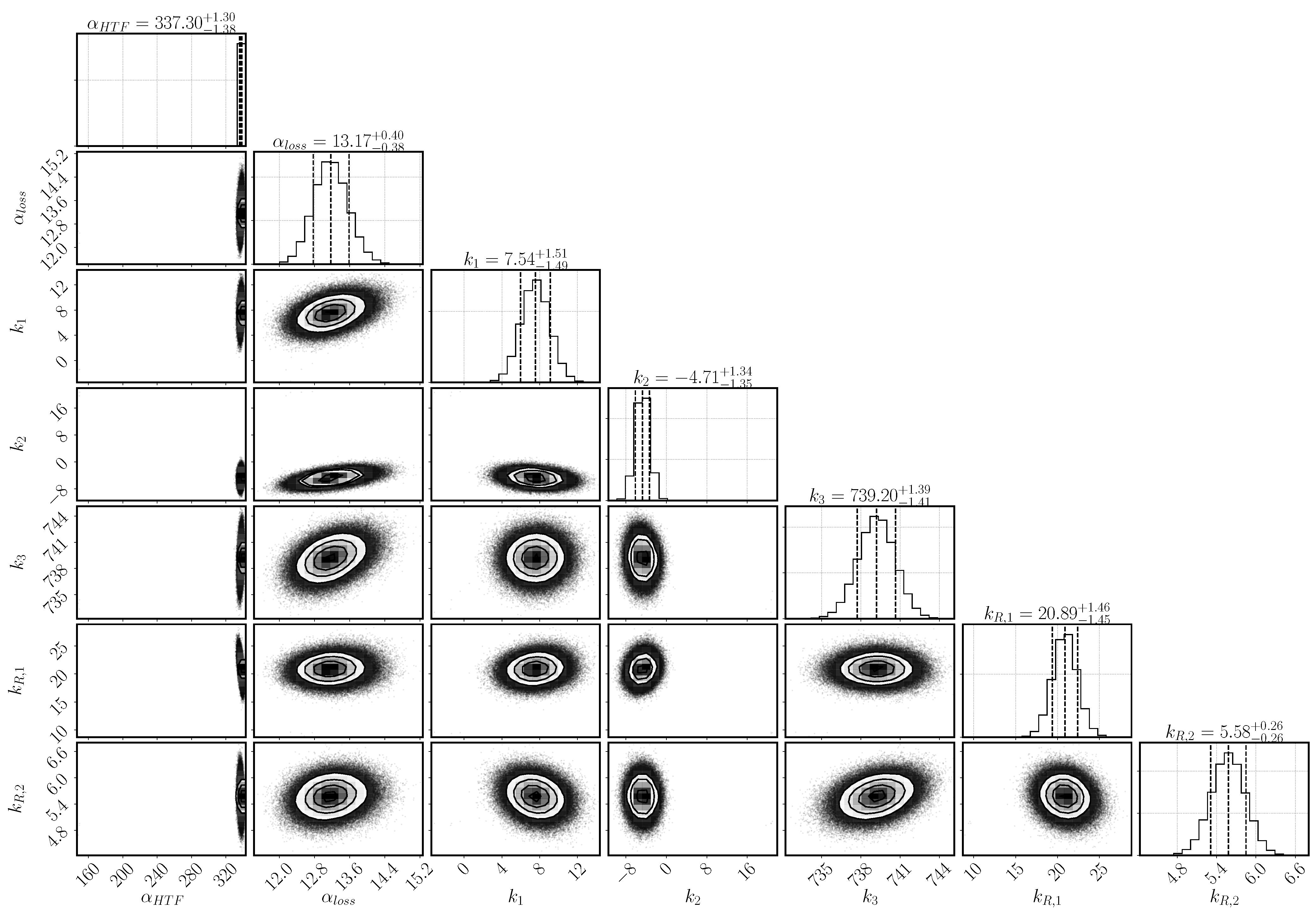
Figure 3 shows the posterior distribution for the parameters and their dependencies. The optimum values and the 95% confidence interval of each parameter are as well listed in

Table 6. Optimized set of parameters with mean 95% confidence interval.

Parameter	Symbol	Unit	Mean	+	−
Heat-transfer coefficient	${\alpha }_{HTF}$	$\mathrm{W}/{\mathrm{m}}^2\mathrm{K}$	337	1.30	1.38
Heat-loss coefficient	${\alpha }_{loss}$	$\mathrm{W}/{\mathrm{m}}^2\mathrm{K}$	13.2	0.40	0.38
Temperature distribution Param1	$k_1$	${\mathrm{Km}}^{-2}$	7.54	1.51	1.49
Temperature distribution Param2	$k_2$	${\mathrm{Km}}^{-1}$	−4.71	1.34	1.35
Temperature distribution Param3	$k_3$	K	739	1.39	1.41
Reaction coeffiecient	$k_{R,1}$	s${}^{-1}$	20.9	1.46	1.45
Reaction exponent	$k_{R,2}$	-	5.58	0.26	0.26

. All the parameters display a Gaussian posterior distribution, that is, the model output is sensitive to all the selected parameters. Otherwise, the posterior distribution would resemble the prior, uniform distribution. The narrower the width of the Gaussian distribution, the more sensitive the model output is on the respective parameter.

The heat-transfer coefficient has a narrow distribution and lies with ${\alpha }_{HTF}=337$ $\mathrm{W}/{\mathrm{m}}^2\mathrm{K}$ as mean value at the upper bond of the selected range. The larger the heat transfer coefficient, the more heat is transported to the heat-transfer channel given the same temperature conditions. The heat transfer is, however, correlated to the heat-loss mechanism that transports the heat to the top of the reactive bed. It is described by the combination of the parameters ${\alpha }_{HTF}$, ${\alpha }_{Loss}$ and k${}_1$–k${}_3$. Both mechanisms depend on the temperature at the boundary of the reactive bed and the outer temperature of both the HTF channel and the vapor vessel. However, the temperature distribution in the HTF channel changes according to the progress of conversion. In early stages, the reaction occurs everywhere in the reactive bed until the local temperature reaches the equilibrium temperature. Afterwards, reaction occurs only where the reaction bed is cooled down. Heat is transported to the HTF channel, where cooler air is injected from the left. The flowing air takes up the heat of the reactive bed. The temperature difference between bed and channel is largest at the inlet and, thus, the reactive material is converted the fastest at this point. Eventually, a reaction front develops between the region, that has already been converted, and the region, where the conditions are still at equilibrium. Only at the front, the conditions of temperature and pressure are such that the chemical reaction can occur. If no heat was lost and all the heat was transported to the HTF channel, the reaction front would move diagonally from the bottom left to the top right corner of the reactive bed. However, heat is also lost at the top boundary dependent on the temperature in the outer vessel and, thus, the reaction is fast also close to the top boundary. In the center of the bed, the front moves slowly and a kind of parabolic shape of the reaction front establishes. The exact shape is not tracked by the experiment, as only the temperatures at location T1, T3, and T7 are measured. The temperature distribution in the vapor vessel is described by the parameters k${}_1$–k${}_3$. Via the temperature profiles at the locations T1, T3 and T7, it is thus inferred how much heat is transferred to the HTF channel or lost to the vapor vessel.

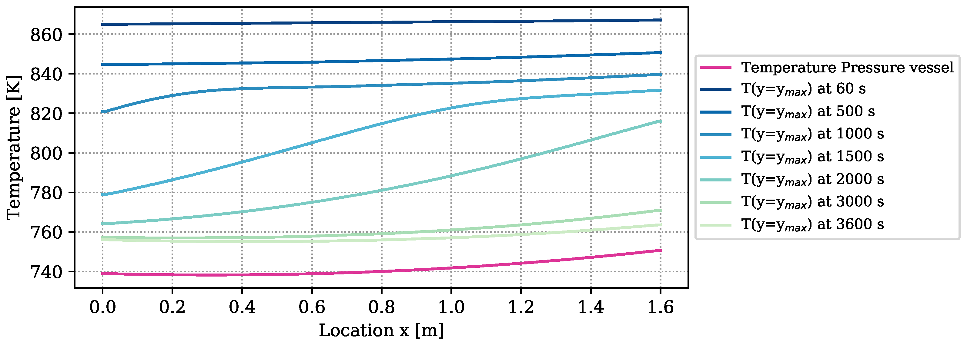
The amount of heat loss is determined by the temperature difference between the boundary of the reactive bed and the vapor vessel, and by the heat loss coefficient. The temperature distribution of the outer vessel is plotted in purple in Figure 4. It furthermore contains the temperatures at the boundary of the reactive bed, $T(y=y_{max}$), determined by a simulation with the numrical model at optimized parameters. The temperature differences between bed and vessel amount to more than 100 K at early times of reaction. At the end of the experiment, they still amount to 20 K. 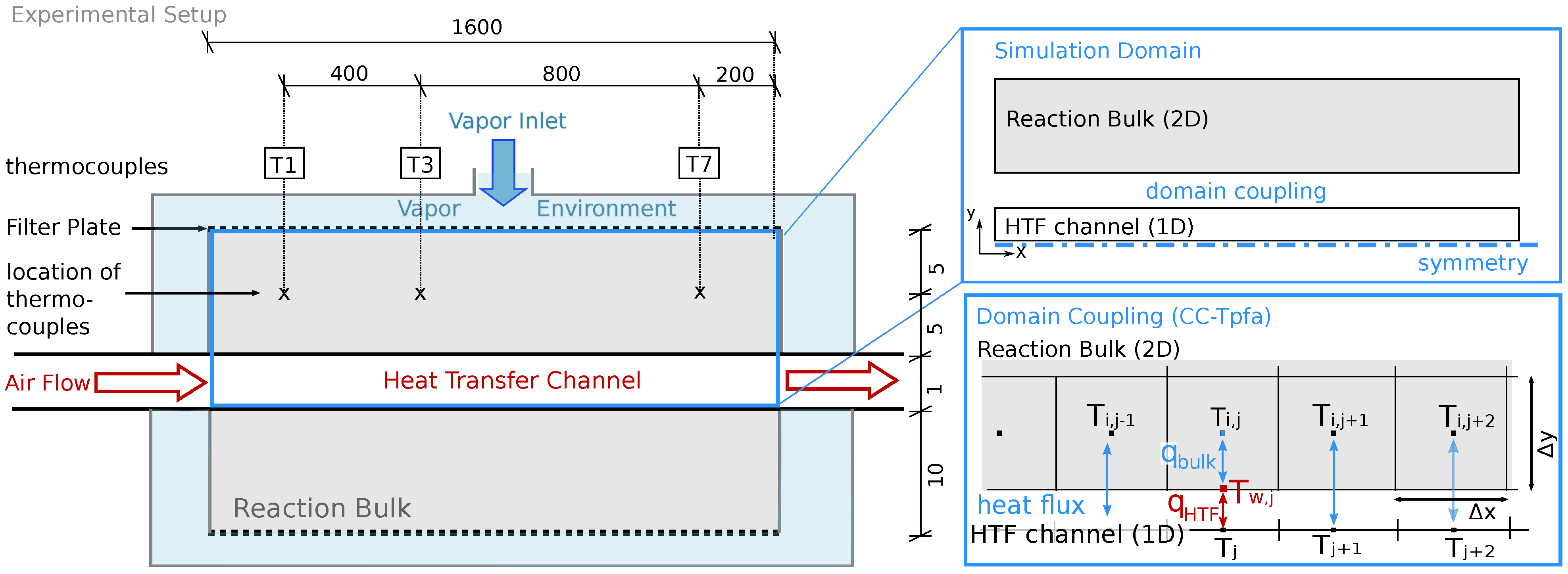Due to the big temperature differences, $1.34\times {10}^3$ $\mathrm{k}\mathrm{J}$ of the overall released energy of reaction ($2.24\times {10}^3$ $\mathrm{k}\mathrm{J}$) is lost through the reactor surface and only $0.93\times {10}^3$$\mathrm{k}\mathrm{J}$ is transferred to the HTF channel. Temperature measurements in the HTF channel to verify these results are not available. The heat-transport mechanisms in form of heat loss, free convection, conduction, and radiation overlap. Free convection, however, appears only at the upper boundary of the symmetric reactor setup, as outlined in Section 2.2.2. If this mechanism dominates the heat loss, the temperatures in the reactive bed below and above the HTF channel are different and the symmetry condition is not fulfilled. In the experiment, all the thermocouples are installed in the top part of the reactive bed. Thus, the experiment does not provide any information on whether or not the two parts behave symmetrically. The reduced simulation domain provides a considerable simulation speed-up.

The parameters k${}_{R,1}$ and k${}_{R,2}$ are linked via the reaction rate. Both a small value of k${}_{R,1}$ and a large value of k${}_{R,2}$ limit the reaction rate and lead to a flat slope in the temperature profiles. The optimal solution is found above the expected ranges for both parameters with k${}_{R,1}=20.9$ and k${}_{R,2}=5.58$. Whereas k${}_{R,1}=20.9$ is only slightly larger than its upper value at 20, k${}_{R,2}=5.58$ is clearly above its range. At initial states of conversion, k${}_{R,2}=5.58$ hardly affects the reaction rate, as the term ${(1-X)}^{k_{R,2}}$ is close to one. Its impact increases with increasing conversion. At medium conversion, the dampening effect is compensated by the high value of k${}_{R,1}$, but at final stages, it dominates the reaction rate. k${}_{R,2}$ in fact prevents complete conversion within the simulation time.

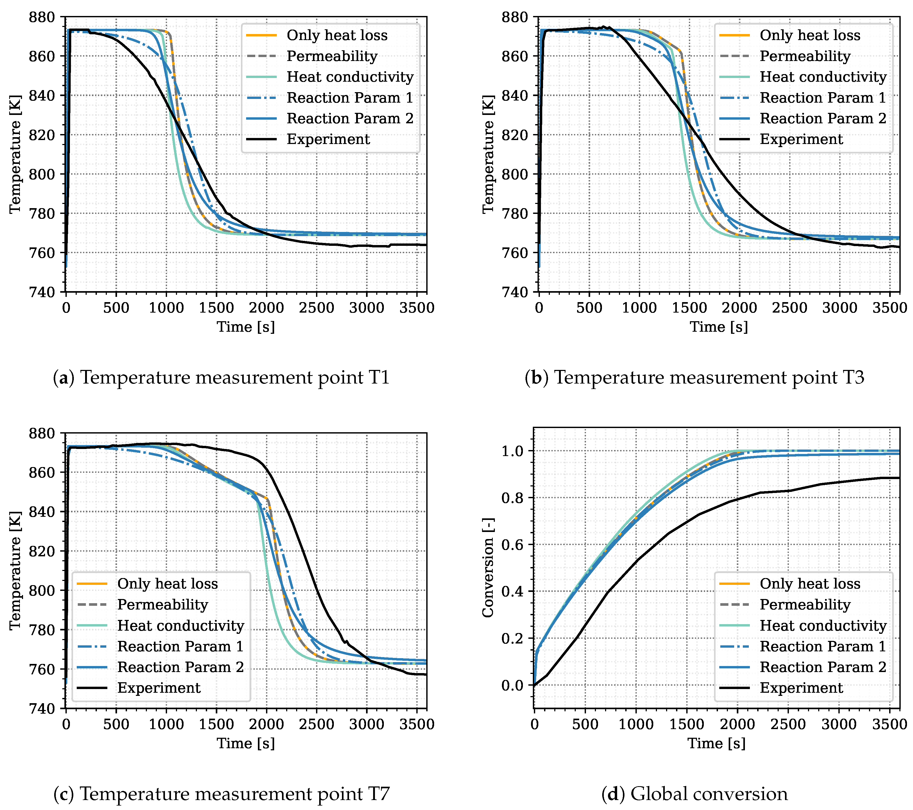
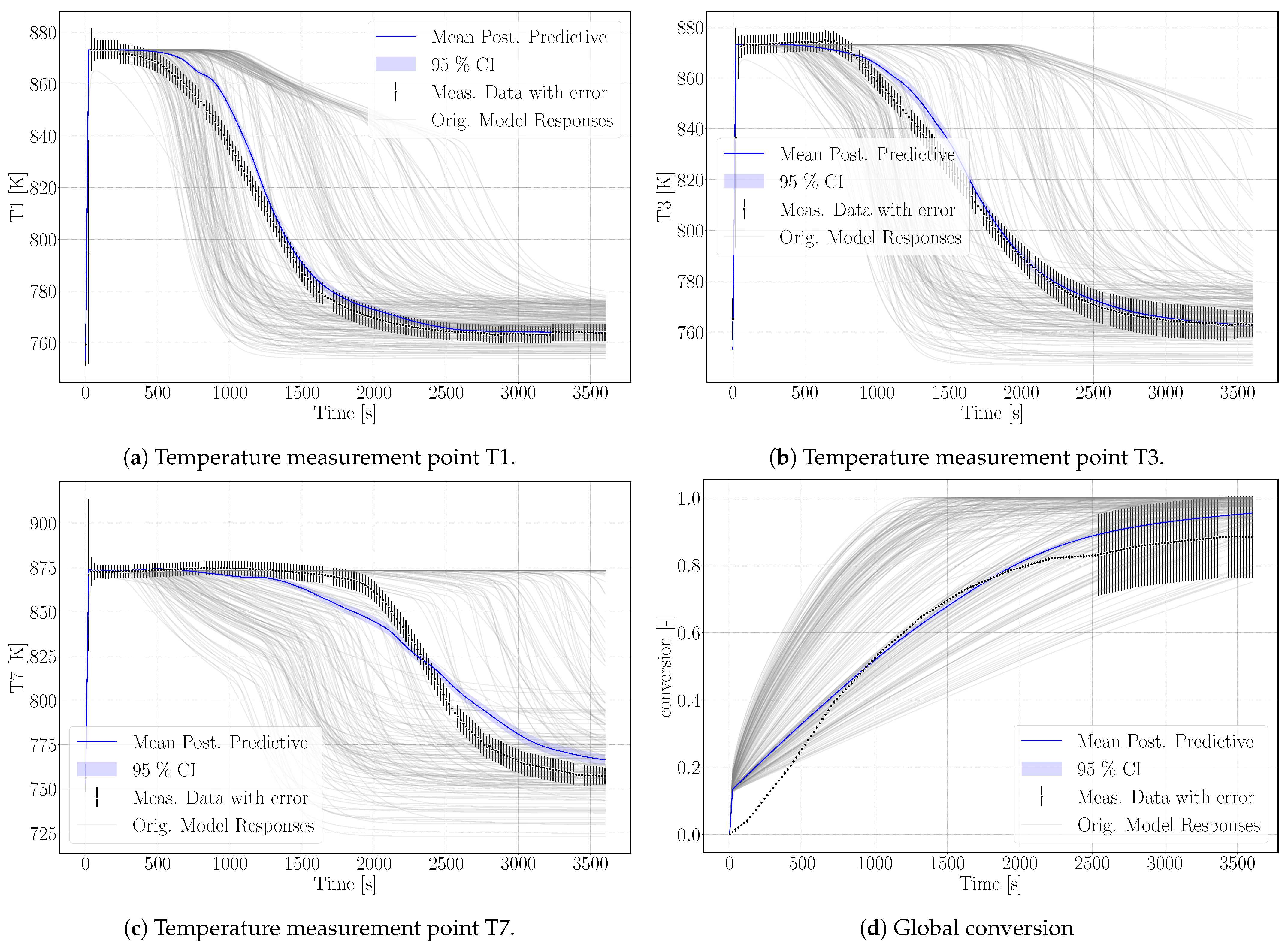
Experimental results and simulation results agree in this regard as shown in Figure 5d. The conversion in the experiment stagnates at 88% and the maximum conversion of the simulation reaches 95% after 3600 s of reaction. A large error was assigned to the experimental values at final stages in order to not exclude complete conversion. Schmidt et al. [32] performed 33 cycles of charging and discharging with the same reactor filling. They reach maximal values of conversion between 90–95% for the duration of the experiments and state that the final 5–10% need significanty more time [31]. Additionally, they detect the formation of agglomerates. Rosskopf et al. [57] show, that the surrounding of the agglomerates form fracture-like preferential flow paths with higher permeability compared to the agglomerates. Schaube et al. [23] state for a directly operated fixed-bed reactor with CaO/Ca(OH)${}_2$, the last 20% of solid bulk get converted slower as soon as agglomerates have been formed. In the reactive bed of the indirectly operated reactor concept, pressure gradients are the result of water consumption due to the chemical reaction. Differences in permeability in the agglomerates and their surroundings result in inhomogeneous pressure gradients. The reactive material close to the preferential flow paths is well supplied with reaction fluid and reacts fast. Less water reaches the solid material within the agglomerates. Here, in a self-enhancing mechanism, a smaller pressure gradient deteriorates the supply of water vapor even further and the reactive solid material reacts slowly. This retardation effect of the agglomerates becomes noticeable with increasing conversion, when the material close to the preferential flow paths has already reacted. The reduced heat production due to the lower reaction rate is overlapped by heat conduction and the slope of the temporal temperature profile is flattened. It is thus deduced that agglomerates retard the reaction rate at progressed conversion also in the indirectly operated reactor concept. The term ${(1-X)}^{k_{R,2}}$ represents the retardation at progressed conversion and describes the effect of the agglomerates phenomenologically. Thus, there is no easy physical interpretation of the parameter k${}_{R,2}$; primarily, it fulfilled the purpose of identifying a relevant phenomenon, so it may only be interpreted qualitatively. As its inferred value is large (k${}_{R,2}$= 5.58), we conclude that the effect of agglomerates is important. If it was not important, k${}_{R,2}$ would have a value close to zero.

The surrogate model represents the conversion profile satisfactorily, see Figure 5d. At the beginning, the simulation overestimates the conversion, as the model does not represent the experimental procedure exactly. The pressure in the vapor vessel was used as initial condition in the reactive bed, whereas in the experiment, the reactor had been evacuated beforehand. However, the initial pressure of the experiment is unknown. The initial water pressure in the simulation setup leads to increased conversion at early simulation stages until the additional water vapor caused by the initial condition is consumed by the reaction. At later times, experimental and simulation results match well, also with respect to incomplete conversion.

Figure 5 shows the simulation results of the surrogate model together with the experimental results for the temperature distributions at T1, T3, T7 and the conversion. The results of the calibrated model indicate a good agreement with the experimental data. In particular, the temperature curves T1 and T3 reflect the temperature profile well, including the slope of decreasing temperature at final conversion and the final temperature after conversion. The discrepancy in T7 is larger. As the reaction front moves from left to right, this measurement point is less determined by initial and boundary conditions. The surrogate model is built based on the 500 DuMu${}^{\mathrm{x}}$-simulations. Thus, the model uncertainties accumulate at this point. This explains furthermore the wavy shape of the surrogate model results for T7. The shape of T1 and T3 is smoother and features a smaller confidence interval especially at later simulation times compared to T7.

5.2. Validation

The calibrated surrogate model was used for simulating the experiment Case R20, see Table 3, with a similar setup but different water vapor pressure ($270\times {10}^5$ Pa) and air volume flux in the HTF channel (47.22 $\mathrm{k}\mathrm{g}/{\mathrm{m}}^2/\mathrm{s}$). The lower water pressure results in a lower equilibrium temperature and, despite a larger heat-transfer flux, in a slower conversion. The experimental data exceed 100% conversion against the statement of Reference [31] that conversions of maximum 95% were reached. We attribute this to measurement uncertainty. 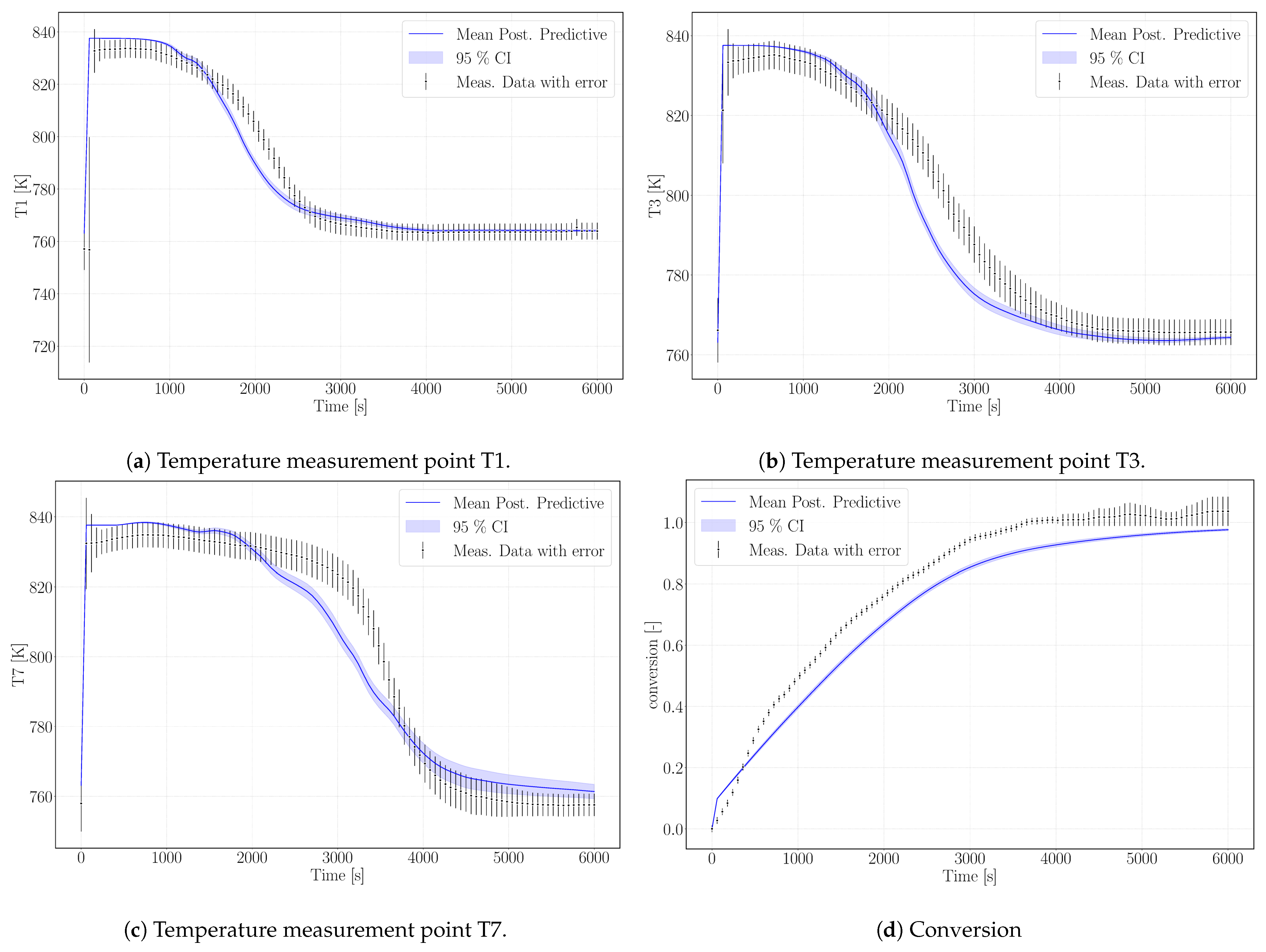Figure 6 shows the simulation results of the surrogate model.

As outlined in the previous section, the simulation does not reach complete conversion due to the high value of the parameter k${}_{R,2}$ that phenomenologically represents the changed reaction dynamics once agglomerates have formed. As the experiment reaches 100% in 6000 s, possibly no agglomerates are present yet. This would be the case, if this experimental run was one of the first in a row of the altogether 33 experiments performed with the same reactor filling [32]. The chronological order of the experiments is not mentioned in References [31,32] or Reference [20]. The parameter k${}_{R,2}$ limits the reaction rate at progressed conversion and the temperature profiles unfold accordingly. Experimental data and simulation results of the temperatures T1, T3, and T7 are shown in Figure 6a–c. The profiles show a good agreement with the experimental temperature curves. Thus, we tend to attribute this to a measurement bias in the experimental data regarding conversion.

The model results overestimate the equilibrium temperature of the experiment. The equilibrium condition for pressure and temperature of Reference [14], which was used for the calibration case, is not adapted to the pressure conditions of the reaction conditions. The simulated temperatures, however, are still in the range of measurement uncertainty. Despite that, the temperature profiles of this experimental setup are reproduced with an accuracy comparable to the calibration case. The decrease in temperature is slightly steeper in the model results, but the velocity of the reaction front matches the model results. The final temperatures for each measurement lay within the range of measurement uncertainty.

6. Conclusions

This study presents a model concept for simulating the indirectly operated reactor concept. It is composed of two subdomains, one for the reactive bed and one for the heat transfer channel. Both submodels are coupled by exchanging a conductive heat flux.

A major objective of this study was the calibration and validation of the numerical model. The simulation results were compared to experimental temperature data at distinct measurement points and to the overall conversion for a discharge reaction as presented in Reference [31]. The temperature in the experiment, however, falls below the temperature imposed in the heat transfer channel. In Reference [20], this was explained with heat losses occuring over the reactor casing. Our study reveals that introducing the hypothesized heat loss in the model concept is not sufficient to reproduce the experimental temperature profiles. Another important mechanism could be identified and is concerned with the decrease in the reaction rate with increasing conversion of the reactive material. To represent this effect phenomenologically in our model, we modified the reaction kinetics by introducing the factor ${(1-X)}^{k_{R,2}}$.

With the heat-transfer coefficient in the heat transfer channel, the temperature distribution outside of the reactive bed, the heat-loss coefficient, and two reaction-rate constants, we identified altogether seven model parameters as relevant to be included in a calibration for the envisaged simulation setup. They were inferred with the help of Bayesian inversion based on a Markov chain Monte Carlo algorithm. To accelerate the process, we replaced the numerical model by a PCE (polynomial chaos expansion) surrogate model that we trained with 500 simulation runs at varying parameters covering the parameter space. The Bayesian inference delivers a posterior parameter distribution with the mean being the most probable value. All the inferred parameters were Gaussian distributed in the posterior distribution. This confirms that our numerical model is sensitive to all of them. The simulation results of the calibrated surrogate model showed a good match with the measurements. A subsequent validation with a similar experiment at different boundary conditions confirms the model for the experimental setup.

The new insights from this modelling study into the interpretation of the experimental temperature data and the conversion rates of the reactive material can be summarized as follows:

In addition to the heat transported in the heat transfer channel, heat is lost over the reactor surface. As temperatures close to the equilibrium temperature limit the reaction, the heat losses in fact lead to an increased speed of reaction. A temperature difference between the surface of the reactive bed and the casing of the vapor vessel induces a heat transport by a combination of different heat-transport processes, notably heat conduction, free convection, and radiation. It is beyond the scope of our study to identify the amount of heat loss associated to each mechanism separately. But we inferred that with $1.34\times {10}^3$ $\mathrm{k}\mathrm{J}$ in total more heat is lost over the reactor surface than transported to the heat transfer channel ($0.93\times {10}^3$ $\mathrm{k}\mathrm{J}$).

Contrary to the statement of Reference [20] that the experimental results can be reproduced by only considering the heat losses occuring in the homogeneous reactive bed, we identified an additional process that requires consideration. Our results indicate that the agglomerates decelerate the reaction in the reactive bed of the indirectly operated reactor, as they limit the distribution of the reaction fluid. We represented this effect phenomenologically by modifying the reaction kinetics. A reduced reaction rate at later stages of progressed conversion permits reaching the equilibrium temperature at the beginning of the reaction and causes a flatter slope of the temperature jump at the end of conversion. Due to the retardation of the reaction, no complete conversion is reached then within the given duration of the experiment. This is confirmed by the experimental data on the course of conversion.

Perspectively, these findings can be used to further elaborate on the process details regarding the agglomerates, which we addressed only phenomenologically. For example, one may apply a double-porosity model. However, such a model involves further model parameters that need to be determined in well-designed joint experimental and numerical studies.

References

1. Parameshwaran, R.; Kalaiselvam, S.; Harikrishnan, S.; Elayaperumal, A. Sustainable thermal energy storage technologies for buildings: A review. Renew. Sustain. Energy Rev. 2012, 16, 2394–2433. [Google Scholar] [CrossRef]
2. N’Tsoukpoe, K.E.; Schmidt, T.; Rammelberg, H.U.; Watts, B.A.; Ruck, W.K. A systematic multi-step screening of numerous salt hydrates for low temperature thermochemical energy storage. Appl. Energy 2014, 124, 1–16. [Google Scholar] [CrossRef]
3. Yan, T.; Wang, R.; Li, T.; Wang, L.; Fred, I.T. A review of promising candidate reactions for chemical heat storage. Renew. Sustain. Energy Rev. 2015, 43, 13–31. [Google Scholar] [CrossRef]
4. Richter, M.; Habermann, E.M.; Siebecke, E.; Linder, M. A systematic screening of salt hydrates as materials for a thermochemical heat transformer. Thermochim. Acta 2018, 659, 136–150. [Google Scholar] [CrossRef]
5. Chacartegui, R.; Alovisio, A.; Ortiz, C.; Valverde, J.; Verda, V.; Becerra, J. Thermochemical energy storage of concentrated solar power by integration of the calcium looping process and a CO2 power cycle. Appl. Energy 2016, 173, 589–605. [Google Scholar] [CrossRef]
6. Qu, X.; Li, Y.; Li, P.; Wan, Q.; Zhai, F. The development of metal hydrides using as concentrating solar thermal storage materials. Front. Mater. Sci. 2015, 9, 317–331. [Google Scholar] [CrossRef]
7. Block, T.; Schmücker, M. Metal oxides for thermochemical energy storage: A comparison of several metal oxide systems. Sol. Energy 2016, 126, 195–207. [Google Scholar] [CrossRef]
8. Schaube, F.; Koch, L.; Wörner, A.; Müller-Steinhagen, H. A thermodynamic and kinetic study of the de-and rehydration of Ca(OH)2 at high H2O partial pressures for thermo-chemical heat storage. Thermochim. Acta 2012, 538, 9–20. [Google Scholar] [CrossRef]
9. Angerer, M.; Becker, M.; Härzschel, S.; Kröper, K.; Gleis, S.; Vandersickel, A.; Spliethoff, H. Design of a MW-scale thermo-chemical energy storage reactor. Energy Rep. 2018, 4, 507–519. [Google Scholar] [CrossRef]
10. Schmidt, M.; Linder, M.P. Thermochemical energy storage for seasonal balance of surplus electricity and heat in domestic buildings. In Proceedings of the Internation Conference on Solar Energy for Buildings and Industry, Palma, Mallorca, 8–17 May 2016. [Google Scholar]
11. Angerer, M.; Djukow, M.; Riedl, K.; Gleis, S.; Hartmut, S. Simulation of Cogeneration-Combined Cycle Plant Flexibilization by Thermochemical Energy Storage. J. Energy Resour. Technol. 2017, 140. [Google Scholar] [CrossRef] [Green Version]
12. Rougé, S.; Criado, Y.A.; Huille, A.; Abanades, J.C. Proof of concept of the CaO/Ca(OH)2 reaction in a continuous heat-exchanger BFB reactor for thermochemical heat storage in CSP plants. AIP Conf. Proc. 2017, 1850, 090005. [Google Scholar] [CrossRef] [Green Version]
13. Rosemary, J.K.; Bauerle, G.L.; Springer, T.H. Solar Energy Storage Using Reversible Hydration-Dehydration of CaO-Ca(OH)2. J. Energy 1979, 3, 321–322. [Google Scholar] [CrossRef]
14. Samms, J.A.C.; Evans, B.E. Thermal dissociation of Ca(OH)2 at elevated pressures. J. Appl. Chem. 1968, 18, 5–8. [Google Scholar] [CrossRef]
15. Lin, S.; Harada, M.; Suzuki, Y.; Hatano, H. CaO Hydration Rate at High Temperature (∼1023 K). Energy Fuels 2006, 20, 903–908. [Google Scholar] [CrossRef]
16. Criado, Y.A.; Alonso, M.; Abanades, J.C. Kinetics of the CaO/Ca(OH)2 hydration/dehydration reaction for thermochemical energy storage applications. Ind. Eng. Chem. Res. 2014, 53, 12594–12601. [Google Scholar] [CrossRef] [Green Version]
17. Irabien, A.; Viguri, J.R.; Ortiz, I. Thermal dehydration of calcium hydroxide. 1. Kinetic model and parameters. Ind. Eng. Chem. Res. 1990, 29, 1599–1606. [Google Scholar] [CrossRef]
18. Schmidt, M. Experimental Investigation of Ca(OH)2 as Thermochemical Energy Storage at Process Relevant Boundary Conditions. Ph.D. Thesis, University of Stuttgar, Stuttgart, Germany, 2017. [Google Scholar]
19. Nagel, T.; Shao, H.; Roßkopf, C.; Linder, M.; Wörner, A.; Kolditz, O. The influence of gas–solid reaction kinetics in models of thermochemical heat storage under monotonic and cyclic loading. Appl. Energy 2014, 136, 289–302. [Google Scholar] [CrossRef]
20. Risthaus, K.; Bürger, I.; Linder, M.; Schmidt, M. Numerical analysis of the hydration of calcium oxide in a fixed bed reactor based on lab-scale experiments. Appl. Energy 2020, 261, 114351. [Google Scholar] [CrossRef]
21. Schmidt, P. On the Design of a Reactor for High Temperature Heat Storage by Means of Reversible Chemical Reactions. Master’s Thesis, KTH School of Industrial Engineering an Management, Stockholm, Sweden, 2011. [Google Scholar]
22. Michel, B.; Mazet, N.; Mauran, S.; Stitou, D.; Xu, J. Thermochemical process for seasonal storage of solar energy: Characterization and modeling of a high density reactive bed. Energy 2012, 47, 553–563. [Google Scholar] [CrossRef] [Green Version]
23. Schaube, F.; Kohzer, A.; Schütz, J.; Wörner, A.; Müller-Steinhagen, H. De- and rehydration of Ca(OH)2 in a reactor with direct heat transfer for thermo-chemical heat storage. Part A: Experimental results. Chem. Eng. Res. Des. 2013, 91, 856–864. [Google Scholar] [CrossRef]
24. Linder, M.; Roßkopf, C.; Schmidt, M.; Wörner, A. Thermochemical energy storage in kW-scale based on CaO/Ca(OH)2. Energy Procedia 2014, 49, 888–897. [Google Scholar] [CrossRef] [Green Version]
25. Nagel, T.; Beckert, S.; Lehmann, C.; Gläser, R.; Kolditz, O. Multi-physical continuum models of thermochemical heat storage and transformation in porous media and powder beds—A review. Appl. Energy 2016, 178, 323–345. [Google Scholar] [CrossRef]
26. Shao, H.; Nagel, T.; Roßkopf, C.; Linder, M.; Wörner, A.; Kolditz, O. Non-equilibrium thermo-chemical heat storage in porous media: Part 2—A 1D computational model for a calcium hydroxide reaction system. Energy 2013, 60, 271–282. [Google Scholar] [CrossRef]
27. Ranjha, Q.; Oztekin, A. Numerical analyses of three-dimensional fixed reaction bed for thermochemical energy storage. Renew. Energy 2017, 111, 825–835. [Google Scholar] [CrossRef]
28. Seitz, G.; Helmig, R.; Class, H. A numerical modeling study on the influence of porosity changes during thermochemical heat storage. Appl. Energy 2020, 259, 114152. [Google Scholar] [CrossRef]
29. Balasubramanian, G.; Ghommem, M.; Hajj, M.R.; Wong, W.P.; Tomlin, J.A.; Puri, I.K. Modeling of thermochemical energy storage by salt hydrates. Int. J. Heat Mass Transf. 2010, 53, 5700–5706. [Google Scholar] [CrossRef]
30. Schaube, F.; Utz, I.; Wörner, A.; Müller-Steinhagen, H. De- and rehydration of Ca(OH)2 in a reactor with direct heat transfer for thermo-chemical heat storage. Part B: Validation of model. Chem. Eng. Res. Des. 2013, 91, 865–873. [Google Scholar] [CrossRef]
31. Schmidt, M.; Linder, M. Power generation based on the Ca(OH)2/CaO thermochemical storage system—Experimental investigation of discharge operation modes in lab scale and corresponding conceptual process design. Appl. Energy 2017, 203, 594–607. [Google Scholar] [CrossRef]
32. Schmidt, M.; Gutierrez, A.; Linder, M. Thermochemical energy storage with CaO/Ca(OH)2—Experimental investigation of the thermal capability at low vapor pressures in a lab scale reactor. Appl. Energy 2017, 188, 672–681. [Google Scholar] [CrossRef]
33. Bear, J. Modeling Phenomena of Flow and Transport in Porous Media; Springer eBook Collection. Earth and Environmental Science; Springer: Cham, Switzerland, 2018; Volume 31. [Google Scholar]
34. Helmig, R. Multiphase Flow and Transport Processes in the Subsurface: A Contribution to the Modeling of Hydrosystems; Springer: Berlin/Heidelberg, Germany, 1997. [Google Scholar]
35. Nagel, T.; Ostermeier, P.; Seitz, G.; Class, H.; Helmig, R. THC-Processes. In Thermo-Hydro-Mechanical-Chemical Processes in Fractured Porous Media: Modelling and Benchmarking; Kolditz, O., Nagel, T., Shao, H., Wang, W., Bauer, S., Eds.; Springer: Cham, Switzerland, 2018. [Google Scholar] [CrossRef]
36. Incropera, F.P.V. (Ed.) Foundations of Heat Transfer, 6th ed.; Wiley: Hoboken, NJ, USA, 2013; p. 23. [Google Scholar]
37. Gnielinski, V. Heat Transfer in Concentric Annular and Parallel Plate Ducts; VDI Heat Atlas; Springer: Berlin/Heidelberg, Germany, 2010; Chapter G1; pp. 701–708. [Google Scholar]
38. White, F.M. Fluid Mechanics, 8th ed.; McGraw-Hill Series in Mechanical Engineering; McGraw-Hill Education: New York, NY, USA, 2016; p. 14. [Google Scholar]
39. Mokheimer, E.M. Performance of annular fins with different profiles subject to variable heat transfer coefficient. Int. J. Heat Mass Transf. 2002, 45, 3631–3642. [Google Scholar] [CrossRef]
40. Langeheinecke, K.; Kaufmann, A.; Langeheinecke, K.J.; Thieleke, G.; Langeheinecke, K. Thermodynamik für Ingenieure: Ein Lehr-und Arbeitsbuch für das Studium, 10th ed.; Springer: Wiesbaden, Germany, 2017. [Google Scholar]
41. Koch, T.; Gläser, D.; Weishaupt, K.; Ackermann, S.; Beck, M.; Becker, B.; Burbulla, S.; Class, H.; Coltman, E.; Emmert, S.; et al. DuMux 3—An open-source simulator for solving flow and transport problems in porous media with a focus on model coupling. Comput. Math. Appl. 2020. [Google Scholar] [CrossRef]
42. Haynes, W.M.H. (Ed.) CRC Handbook of Chemistry and Physics: A Ready-Reference Book of Chemical and Physical Data; CRC: Boca Raton, FL, USA, 2011; Volume 91. [Google Scholar]
43. Robert, C.; Casella, G. Monte Carlo Statistical Methods; Springer Science & Business Media: Berlin/Heidelberg, Germany, 2013. [Google Scholar]
44. Liu, J.S. Monte Carlo Strategies in Scientific Computing; Springer Science & Business Media: Berlin/Heidelberg, Germany, 2008. [Google Scholar]
45. Wagner, P.R.; Nagel, J.; Marelli, S.; Sudret, B. UQLab User Manual—Bayesian Inversion for Model Calibration and Validation; Technical, Report; Chair of Risk, Safety and Uncertainty Quantification; ETH Zurich: Zurich, Switzerland, 2019; Report # UQLab-V1.3-113. [Google Scholar]
46. Metropolis, N.; Rosenbluth, A.W.; Rosenbluth, M.N.; Teller, A.H.; Teller, E. Equation of state calculations by fast computing machines. J. Chem. Phys. 1953, 21, 1087–1092. [Google Scholar] [CrossRef] [Green Version]
47. Hastings, W.K. Monte Carlo sampling methods using Markov chains and their applications. Biometrika 1970, 57, 97–109. [Google Scholar] [CrossRef]
48. Goodman, J.; Weare, J. Ensemble samplers with affine invariance. Commun. Appl. Math. Comput. Sci. 2010, 5, 65–80. [Google Scholar] [CrossRef]
49. Allison, R.; Dunkley, J. Comparison of sampling techniques for Bayesian parameter estimation. Mon. Not. R. Astron. Soc. 2014, 437, 3918–3928. [Google Scholar] [CrossRef] [Green Version]
50. Wicaksono, D.C. Bayesian Uncertainty Quantification of Physical Models in Thermal-Hydraulics System Codes; Technical Report; EPFL: Lausanne, Switzerland, 2018. [Google Scholar]
51. Foreman-Mackey, D.; Farr, W.M.; Sinha, M.; Archibald, A.M.; Hogg, D.W.; Sanders, J.S.; Zuntz, J.; Williams, P.K.; Nelson, A.R.; de Val-Borro, M.; et al. emcee v3: A Python ensemble sampling toolkit for affine-invariant MCMC. arXiv 2019, arXiv:1911.07688. [Google Scholar] [CrossRef] [Green Version]
52. Cowles, M.K.; Carlin, B.P. Markov chain Monte Carlo convergence diagnostics: A comparative review. J. Am. Stat. Assoc. 1996, 91, 883–904. [Google Scholar] [CrossRef]
53. Goodman, J. Acor, Statistical Analysis of a Time Series. 2009. Available online: https://www.math.nyu.edu/faculty/goodman/software/acor/ (accessed on 1 December 2020).
54. Domesová, S.; Béreš, M. A Bayesian approach to the identification problem with given material interfaces in the Darcy flow. In Proceedings of the International Conference on High Performance Computing in Science and Engineering, Karolinka, Czech Republic, 22–25 May 2017; pp. 203–216. [Google Scholar]
55. Oberkampf, W.L.; Roy, C.J. Verification and Validation in Scientific Computing; Cambridge University Press: Cambridge, MA, USA, 2010. [Google Scholar]
56. Roy, C.J. Errors and Uncertainties: Their Sources and Treatment. In Computer Simulation Validation; Springer: Berlin/Heidelberg, Germany, 2019; pp. 119–141. [Google Scholar]
57. Roßkopf, C.; Haas, M.; Faik, A.; Linder, M.; Wörner, A. Improving powder bed properties for thermochemical storage by adding nanoparticles. Energy Convers. Manag. 2014, 86, 93–98. [Google Scholar] [CrossRef]
58. Oladyshkin, S.; Nowak, W. Data-driven uncertainty quantification using the arbitrary polynomial chaos expansion. Reliab. Eng. Syst. Saf. 2012, 106, 179–190. [Google Scholar] [CrossRef]
59. Marelli, S.; Sudret, B. UQLab User Manual–Polynomial Chaos Expansions; UQLab-V1.3-113, Chair of Risk, Safety & Uncertainty Quantification; ETH Zurich: Zurich, Switzerland, 2015; pp. 97–110. [Google Scholar]
60. Sudret, B. Uncertainty Propagation and Sensitivity Analysis in Mechanical Models—Contributions to Structural Reliability and Stochastic Spectral Methods; Université Blaise Pascal: Clermont-Ferrand, France, 2007; p. 18. [Google Scholar]
61. Tipping, M.E.; Faul, A.C. Fast marginal likelihood maximisation for sparse Bayesian models. In Proceedings of the Ninth International Workshop on ArtificialIntelligence and Statistics, Key West, FL, USA, 3–6 January 2003. [Google Scholar]
62. Tipping, M.E. Sparse Bayesian learning and the relevance vector machine. J. Mach. Learn. Res. 2001, 1, 211–244. [Google Scholar]
63. Berger, J.O. Statistical Decision Theory and Bayesian Analysis; Springer Science & Business Media: Berlin/Heidelberg, Germany, 2013. [Google Scholar]
64. Gull, S.F. Developments in maximum entropy data analysis. In Maximum Entropy and Bayesian Methods; Springer: Berlin/Heidelberg, Germany, 1989; pp. 53–71. [Google Scholar]
65. MacKay, D.J. Bayesian interpolation. Neural Comput. 1992, 4, 415–447. [Google Scholar] [CrossRef]
66. Nagel, J.B.; Rieckermann, J.; Sudret, B. Principal component analysis and sparse polynomial chaos expansions for global sensitivity analysis and model calibration: Application to urban drainage simulation. Reliab. Eng. Syst. Saf. 2020, 195, 106737. [Google Scholar] [CrossRef] [Green Version]
67. Higdon, D.; Gattiker, J.; Williams, B.; Rightley, M. Computer model calibration using high-dimensional output. J. Am. Stat. Assoc. 2008, 103, 570–583. [Google Scholar] [CrossRef] [Green Version]
Figure 1. Reactor setup; Left: Experimental setup described in Reference [32]. The solid bulk is kept between filter plates. Water is provided at constant pressure in the surrounding casing. Air flows through the heat transfer channel (HTF) to provide/remove heat. Thermocouples are placed at different locations, here T1, T3 and T7. For better visibility, the figure is not true to scale. The dimensions are given in mm. Top right: In the model, the setup consists of two separate domains, the reactive bulk and the (HTF). The two domains are coupled by a conductive heat flux. Due to symmetry, only half of the bulk domain is simulated. Bottom right: Domain coupling; a heat flux is calculated between the cell centers of the two-dimensional reaction bulk and the 1D HTF channel.
Applsci 11 00682 g001
Figure 2. Preliminary simulation results to identify the optimization parameters. In black: experimental values from Reference [31] as reference; Simulation cases: “Only heat loss” is simulated with the standard parameters at constant permeability. “Permeability” applies a permeability change due to porosity alteration, “Heat conductivity” uses different values for solid heat conductivity for CaO and Ca(OH) 2 , “Reaction Param 1” applies a reduced reaction rate constant and “Reaction Param 2” introduces the constant term k R , 2 to the reaction kinetics. The parameters for each simulation case are listed in Table 4.
Applsci 11 00682 g002
Figure 3. Histogramms for the parameter distribution after inverse modeling based on the experimental data of Reference [31]. On the diagonal are the histograms for the single parameters including mean and 95% confidence interval (indicated by the dashed lines). The scatter plots show the covariance between the parameters of the respective row and column.
Applsci 11 00682 g003
Figure 4. Temperature distribution of the outer pressure vessel according to the parameters k 1 –k 3 and at the top boundary of the reactive bed over the reactor length at different times simulated with the DuMu x -model with the parameters of Table 6.
Applsci 11 00682 g004
Figure 5. Simulation results of the calibrated surrogate model with its 95% confidence interval (CI); the surrogate model is based on 200 simulation runs of the numerical model plotted in gray. The experimental reference data are plotted in black including error-bars representing the uncertainties.
Applsci 11 00682 g005
Figure 6. Simulation results (blue) for model validation according to the experimental data of Case R20.
Applsci 11 00682 g006