Article

Numerical Simulation on Spatial-Frequency Domain Imaging for Estimating Optical Absorption and Scattering Properties of Two-Layered Horticultural Products

1
School of Engineering, Zhejiang A&F University, Hangzhou 311300, China
2
College of Mechanical and Electronic Engineering, Nanjing Forestry University, Nanjing 210037, China
3
Hangzhou Doubltech Electro-Hydraulic Engineering Co., Ltd., Hangzhou 310051, China
4
College of Biosystems Engineering and Food Science, Zhejiang University, Hangzhou 310058, China
5
Key Laboratory of on Site Processing Equipment for Agricultural Products, Ministry of Agriculture and Rural Affairs, Zhejiang University, Hangzhou 310058, China
*
Authors to whom correspondence should be addressed.
Appl. Sci. 2021, 11(2), 617; https://doi.org/10.3390/app11020617
Submission received: 9 December 2020 / Revised: 6 January 2021 / Accepted: 7 January 2021 / Published: 10 January 2021
(This article belongs to the Special Issue Applications of Modeling and Simulation in Food Engineering)

Abstract

:
Spatial-frequency domain imaging (SFDI) is a wide-field, noncontact, and label-free imaging modality that is currently being explored as a new means for estimating optical absorption and scattering properties of two-layered turbid materials. The accuracy of SFDI for optical property estimation, however, depends on light transfer model and inverse algorithm. This study was therefore aimed at providing theoretical analyses of the diffusion model and inverse algorithm through numerical simulation, so as to evaluate the potential for estimating optical absorption and reduced scattering coefficients of two-layered horticultural products. The effect of varying optical properties on reflectance prediction was first simulated, which indicated that there is good separation in diffuse reflectance over a large range of spatial frequencies for different reduced scattering values in the top layer, whereas there is less separation in diffuse reflectance for different values of absorption in the top layer, and even less separation for optical properties in the bottom layer. To implement the nonlinear least-square method for extracting the optical properties of two-layered samples from Monte Carlo-generated reflectance, five curve fitting strategies with different constrained parameters were conducted and compared. The results confirmed that estimation accuracy improved as fewer variables were to be estimated each time. A stepwise method was thus suggested for estimating optical properties of two-layered samples. Four factors influencing optical property estimation of the top layer, which is the basis for accurately implementing the stepwise method, were investigated by generating absolute error contour maps. Finally, the relationship between light penetration depth and spatial frequency was studied. The results showed that penetration depth decreased with the increased spatial frequency and also optical properties, suggesting that appropriate selection of spatial frequencies for a stepwise method to estimate optical properties from two-layered samples provides potential for estimation accuracy improvement. This work lays a foundation for improving optical property estimation of two-layered horticultural products using SFDI.

1. Introduction

Optical absorption (μa) and reduced scattering coefficients (μs′) are closely related to tissue physicochemical properties (e.g., tissue porosity, particle size distribution, etc.), which, in turn, could be used as a means for enhancing the nondestructive quality and safety evaluation (e.g., firmness, soluble solids content, titratable acidity, etc.) of horticultural products. In the last two decades, measuring optical properties (i.e., μa and μs′) of horticultural products (e.g., apple, citrus and tomato) have been widely studied by different researchers in the field of food and agricultural engineering [1,2,3]. It was reported that the multiplication of absorption and reduced scattering coefficients of tomato tissues measured by spatially-resolved techniques were highly correlated with flesh firmness, with a correlation coefficient of 0.835 [1]. In the study of Vanoli et al. (2020) [3], absorption and reduced scattering coefficients of ‘Braeburn’ apples were determined, which were used to evaluate the ripening processes during the shelf life period, as absorption phenomena were related to changes in pigments present in the fruit flesh and peel, while scattering events mirrored changes in the flesh texture.
Most research teams treated the samples as homogeneous media and neglected the difference of optical properties among different layers for simplifying parameter estimation procedure. However, this simplification could bring errors in studying the optical properties, as well as the loss of critical physicochemical information for individual layers. Efforts have been made on developing two- and multi-layered models for measuring μa and μs′ of each layer in the traverse direction (i.e., along the surface of a turbid sample) [4,5,6,7], but the estimation errors reported in most studies are still too large and unacceptable, especially for the second or bottom layer. For example, Cen and Lu (2009) estimated the optical properties of two-layered turbid materials simultaneously by using spatially-resolved techniques [5]. The results showed that absorption and reduced scattering coefficients of the top layer of the model samples were determined with errors within 23.0 and 18.4%, respectively, while the inverse algorithm did not give acceptable estimations for the bottom layer. Weber et al. (2009) applied the technique of spatial-frequency domain imaging (SFDI) to estimate optical properties of layered tissues, and reported average accuracies of ±2 and ±17% for absorption and reduced scattering coefficients of the top layer, respectively, by using the four-parameter fit [8]. However, the estimation errors for absorption coefficients of the bottom layer were as large as ±25%, and no acceptable estimations for the bottom-layer’s reduced scattering coefficients, even with the two-parameter fit. The major reason causing the large estimation error is the much more complex inverse algorithm for a two-layered model since it has five optical parameters (i.e., μa and μs′ of each layer, plus the unknown thickness of the top layer). It is, therefore, desirable to understand the intrinsic properties of the two-layered model prior to implementing an inverse algorithm for optical property estimation. Cen and Lu (2009) conducted sensitivity analysis to study the effects of optical parameters (μa1, μs1′, μa2, μs2′ and Rd, where subscripts 1 and 2 refer to the top and bottom layer, and Rd is diffuse reflectance) in a two-layered model on optical property estimation by using spatially-resolved technique [5], while Wang et al. (2019) studied the effects of five optical parameters (μa1, μs1′, μa2, μs2′ and top-layer thickness d) on reflectance prediction with the technique of spatially-resolved [7]. However, few studies were focused on the theoretical analysis of intrinsic properties of two-layered diffusion model in SFDI for optical property estimations.
As an emerging optical measuring technique, SFDI is capable of noncontact and wide-field mapping of μa and μs′ on a pixel-by-pixel basis, which is absent in other techniques using point light source (e.g., spatially-resolved, time-resolved, and integrating sphere). SFDI can be used for estimating optical properties of homogeneous tissues, as well as layered samples, by using appropriate light transfer models (e.g., diffusion approximation and Monte Carlo). Recently, Tabassum et al. (2018) developed a two-layer look-up-table inversion algorithm for extracting μa and μs′of the bottom layer, in which Monte Carlo simulations were conducted natively in the spatial-frequency domain [9]. The results showed that optical property extractions of the bottom (tumor) layer were determined to be within 20 and 11% of the true values for μa and μs′, respectively. Several other studies have also been reported for estimating μa and μs′ of layered tissues using the SFDI technique [8,9,10,11,12]. Some researchers estimated the four optical properties (μa1, μs1′, μa2 and μs2′) simultaneously with the known top-layer thickness (all-at-once method) [8], while others estimated μa and μs′ of one (often the top) layer first, followed by estimating μa and μs′ of the other layer (stepwise method) [12]. Our previous study demonstrated that the efficacy and accuracy of the stepwise method for estimating optical properties of two-layered samples were superior to that for the all-at-once method, under the constraining conditions for the top-layer thickness between 0.2 and 2.0 mm [13]. In the paper of our recent research, the stepwise method with frequency optimization was employed for measuring the optical properties of apple peel and flesh tissues, and the results showed that there were still relatively large error values (22.8%) for estimating absorption coefficient of the flesh tissue due to the theoretical difficulty in estimating absorption coefficient of the bottom layer [12].
In the stepwise method, accurate measurement of the optical properties of the top layer is critical, because optical property estimations of the bottom layer is based on those of the top layer (i.e., the estimated μa1 and μs1′ are treated as known variables for estimating μa2 and μs2′ with the two-layered diffusion model). Therefore, effects of potential influencing factors, such as relative values of the optical properties of two layers (mfp1′/mfp2′, μa1/μa2 and μs1′/μs2′) and relative values of μs1′ and μa1 (μs1′/μa1) on optical property extraction of the top layer, should be quantitatively described and considered. It should be noted that mfp′ [ = 1/(μa + μs′)] is short for mean free path, which denotes the mean distance of a single step as an energy packet travels within the tissues. Moreover, accurate optical property estimation of two-layered horticultural products with SFDI relies on selecting appropriate curve fitting method, which may have diverse types in terms of free variables. For the two-layered diffusion model that has five unknown variables, the free variable(s) can range from one to five, in principle, depending on the number of constrained parameters. It is expected that evaluation of estimation accuracy of different curve fitting methods would verify that the stepwise method proposed in our previous study has better accuracy than all other curve fitting strategies for estimating optical properties of two-layered samples. In addition, it is preferable to have low light penetration depth when estimating optical properties of the top layer, while high penetration depth is welcome for the bottom layer, due to the fact that detected light should carry more effective information with the target layer. It is reported that light penetration depth in SFDI is closely related to spatial frequency [14]. Hence, it is desirable to quantitatively investigate the relationship between light penetration depth and spatial frequency, in order to improve the optical property estimation of two-layered horticultural products.
This paper presents a theoretical analysis of intrinsic properties of two-layered diffusion model and inverse algorithm through numerical simulation in order to improve optical property estimation using the SFDI technique. Therefore, the objectives of this research were to: (1) explore the effect of optical parameters (μa1, μs1′, μa2 and μs2′) on reflectance prediction; (2) evaluate parameter estimation accuracy of different curve fitting methods for optical property estimations of two-layered samples; (3) investigate potential influencing factors on optical property estimations of the top layer for accurately implementing the stepwise method; (4) study the relationship between light penetration depth and spatial frequency for laying a foundation for frequency optimization.

2. Materials and Methods

2.1. Principle and Diffusion Model

Previous literature has described the principles of SFDI for optical property estimation of turbid media based on diffusion model [13,15], so only a brief description will be provided here. Although not accurate for all optical properties, the diffusion model, which is a simplified form of the radiative transfer equation, remains an efficient tool to model light propagation in turbid media by providing analytical solutions that are easily implemented and intuitive. For a homogeneous one-layered medium of semi-infinite geometry normally illuminated at its surface by a steady-state, planar sinusoidal light pattern, diffuse reflectance at the surface can be yielded by applying the partial-current boundary condition [16]:
R d ( f x ) = 3 A a ( μ e f f / μ t r + 1 ) ( μ e f f / μ t r + 3 A )
where A = 1 R e f f 2 ( 1 + R e f f ) is proportionality constant, R e f f 0.0636 n + 0.668 + 0.71 / n 1.44 / n 2 is the effective reflection coefficient, in which n is the refractive index of the medium, a = μ s / μ t r is the reduced albedo, μ t r = μ a + μ s is the transport coefficient, μa and μs′ are absorption coefficient and reduced scattering coefficient, respectively, μ e f f = ( 3 μ a μ t r + ( 2 π f x ) 2 ) 1 / 2 is the scalar attenuation coefficient, and fx is the spatial frequency.
For a two-layered turbid medium (Figure 1), light within the medium decays exponentially, such that the light source term is different in each layer with the bottom layer being assumed to be infinitely thick. By applying appropriate boundary conditions to the diffusion model, diffuse reflectance at the surface can be expressed using Equation (2) [17]:
R d ( f x ) = A μ s 1 μ e f f 1 A 1 + A 2 A 3 x
where A1, A2 and A3 are constants determined by the boundary conditions, and subscript 1 of μs1′ and μeff1′ refers to the top layer.

2.2. Monte Carlo Simulations

Monte Carlo (MC) offers a flexible and accurate approach for modeling light propagation within tissues [18]. In order to investigate the effects of different optical properties on reflectance prediction from the two-layered diffusion model, to evaluate the estimation accuracy of different curve fitting methods, and to analyze the factors influencing optical property extraction of the top layer, a publicly available MC simulation program for multi-layered turbid media was used [19]. In the simulations, a package of five million photons was tracked. The maximum radial distance of the medium was set to 50 mm, which is large enough to be treated as semi-infinite. The spatial resolution for both radial distance and depth was set to 0.1 mm. The average refractive indices of the two-layered media were both chosen to be 1.35, which was typical for most horticultural products (e.g., apple, blueberry, citrus, tomato etc.) [20,21], while the media above and beneath the tissue were treated as air, with the refractive index of 1.0. The anisotropy factor g was set to 0.9, and Henyey–Greenstein phase function was used to describe light scattering. More details about the phase function can be found in reference by Henyey and Greenstein (1941) [22]. The Monte Carlo multi-layered (MCML) program was first applied to generate the spatially-resolved diffuse reflectance profiles of two-layered samples along the radial distance under the normal incidence of an infinite small light source. Then the 1-D Hankel transform of order zero was used to convert the spatially-resolved reflectance to spatial-frequency domain reflectance [16], which was further used for evaluating the curve fitting methods and investigating the potential influencing factors through optical property estimations.
In this study, a total of 20 combinations of μa and μs′ for two-layered samples (five samples with varying μa or μs′ of each layer with the top-layer thickness of 2 mm, Table S1 in Supplementary Materials) were prepared for investigating the effects of optical properties on reflectance prediction and comparing the estimation accuracy of diverse curve fitting methods. One optical property value was varied, while the other four were held constant. The optical property values for these samples were chosen based on published data [23,24,25], covering a large range of horticultural products with 0.001 mm−1μa ≤ 0.1 mm−1 and 0.5 mm−1μs′≤ 4 mm−1. More simulation samples were created (see Tables S2–S5 in Supplementary Materials for more details) for studying the effects of relative values of the optical properties of two layers (mfp1′/mfp2′, μa1/μa2 and μs1′/μs2′) and relative values of μs1′and μa1 (μs1′/μa1), for optical property extraction from the top layer. The parameters of μa1/μa2 and μs1′/μs2′ were selected for studying the contributions of absorption and reduced scattering coefficients of two layers on estimating optical properties of the top layer, respectively, while mfp1′/mfp2′ was used for studying the combination effect of absorption and reduced scattering coefficients. The diffusion model is based on the assumption that scattering is dominant over absorption (μs′ >> μa), so the parameter of μs1′/μa1 was also selected for investigating its effect on optical property estimation. Hereinafter, these relative values are called influencing factors for convenience. Our previous study has investigated the effect of top-layer thickness on optical property estimation of two-layered medium and also determined the constraining conditions [13], indicating that the top-layer’s maximum thickness could not exceed 2 mm, in order to have acceptable estimations of optical properties of the bottom layer. Hence the top-layer thickness was chosen to be 2 mm for all the simulation samples in this study.

2.3. Inverse Algorithm for Estimating Optical Properties of Two-Layered Samples

Prior to determining the optical properties of two-layered simulation samples from the spatial-frequency domain reflectance, the effect of varied μa and μs′ of each layer on reflectance prediction was investigated, which would be helpful for understanding the two-layered diffusion model. To select the most proper, robust and accurate parameter estimation method for determining the optical properties of two-layered samples, different curve fitting methods that differ in the number of free variables were compared and evaluated (Table 1). First, all five parameters (μa1, μs1′, μa2, μs2′ and d) were estimated simultaneously using the two-layered model in Equation (2) (five-variable fit). Second, the top-layer thickness was assumed to be known and the other four parameters were estimated at once (four-variable fit). Third, μa and μs′ of either the top layer or the bottom layer were estimated, depending on which layer had changed variables, while μa and μs′ of the other layer and thickness the top layer were treated as known (two-variable fit). Fourth, only μa or μs′ was estimated, while all others were treated as known (one-variable fit). Fifth and finally, the one-layered model in Equation (1) was utilized to estimate μa and μs′ of the top layer, which was used in our proposed stepwise method [13]. The estimated optical properties were compared with the true values for evaluating the estimation accuracy.
A nonlinear least-squares fitting method was used to minimize the sum-of-squares of the difference between the true reflectance and predicted reflectance values with estimated parameters using Equation (1) or Equation (2). In this study, a subspace trust-region method based on the interior-reflective Newton approach was used to achieve the algorithm optimization [26], which is defined by minimizing a quadratic function subject to an ellipsoidal constraint. The approach can generate iterates in the strictly feasible region by using a new affine scaling transformation, and the speed of convergence is accelerated by following a reflective line search technique. The optical property estimation procedure from the spatial-frequency domain reflectance of two-layered simulation samples was implemented using the Toolbox function ‘lsqcurvefit’ in Matlab 8.4 (The MathWorks, Inc., Natick, MA, USA). Previous studies revealed that there were inherent discrepancies of the reflectance between the diffusion model and MC simulation, which would greatly affect the accuracy of optical property estimation [16,27]. It was proven that sample-based calibration method could decrease the reflectance discrepancies and improve the estimation accuracy. The method was implemented by first selecting a set of calibration samples depending on the initial estimated values of μs1′. Ratios of diffusion model generated reflectance to MC-generated reflectance for all the calibration samples were obtained, and they were then used for calculating the calibrated reflectance by multiplying the original reflectance for each sample. Since this study is focused on theoretical analysis of a two-layered diffusion model, the sample-based calibration method was thus applied for reflectance correction, which was then used for optical property estimation. More details about the calibration method are referred to Hu et al. (2019) [13].
To qualitatively and quantitatively investigate the factors influencing optical property estimation of the top layer, absolute error contour maps for estimating μa and μs′ were plotted, with the horizontal and vertical axes of the maps denoting start and end spatial frequencies, in which the error was calculated by comparing the true values of μa and μs′ with the parameter estimation results. Eleven start frequencies from 0 to 0.1/mfp1′ with an increment of 0.01/mfp1′ and 18 end frequencies from 0.15/mfp1′ to 0.5/mfp1′ with an increment of 0.02/mfp1′ were evaluated for parameter estimations of the top layer. The interval spacing between each start and end frequency pair was set as 0.01 mm−1. Note that relative errors in contour maps were transformed to absolute values, and the absolute errors of μa and μs′ larger than 60% and 20% were treated as 60% and 20% for better visual effect.

3. Results

3.1. Effect of Varying Optical Properties on Diffuse Reflectance

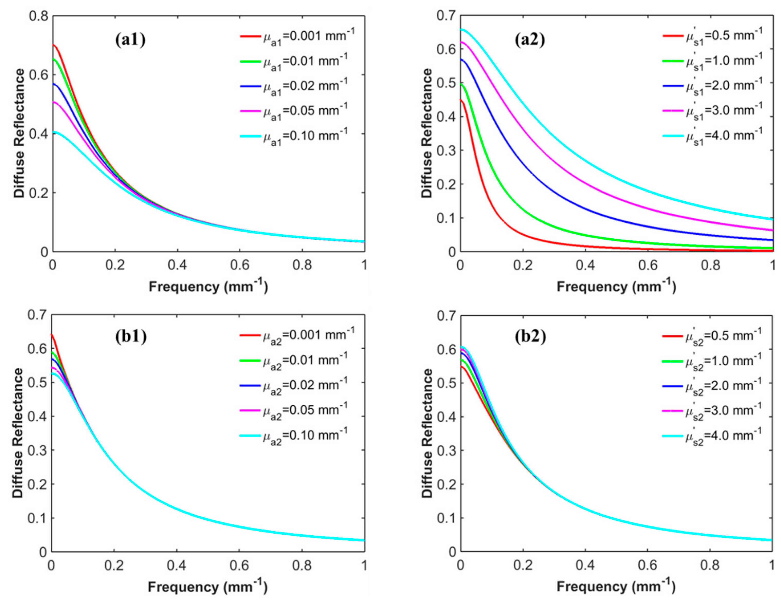
Frequency-dependent diffuse reflectance predicted by the two-layered diffusion model for different optical properties of each layer is plotted in Figure 2; for each plot in the figure one parameter is varied while the other four are held constant. Generally, the reflectance decreased with the increased absorption coefficients, while it increased with the reduced scattering coefficients. The most distinct separation in diffuse reflectance for different values of μa1, μa2 and μs2′ was observed at relatively low frequencies. For varying μs1′ values, the five reflectance curves show distinct differences across the frequency range with the best separation occurring around 0.2 mm−1 (Figure 2(a2)). Overall, Figure 2 demonstrates that there is good separation in diffuse reflectance over a large range of spatial frequencies for different μs1′ values, whereas less separation in diffuse reflectance for different μa1 values, and even less separation for different values of μa2 and μs2′, suggesting the difficulty of accurately estimating the bottom layer. That is because light must propagate through the top layer before interacting with the bottom layer tissue, in which case only a small number of energy packets reemitted from the bottom layer can be detected. In Figure 2(b1,b2), the value of mfp1′ is equal to 0.5 mm, while the top-layer thickness is 2 mm, which implies that light would have travelled more than four steps before entering into the bottom layer. Hence, the separation in diffuse reflectance for different values of μa2 and μs2′ would increase with the decreased top-layer thickness due to the fact that the detected light have more interaction with the bottom layer. The results from the four plots in Figure 2 further suggest that better estimation of the four optical parameters (μa1, μs1′, μa2 and μs2′) could be achieved when low spatial frequencies are used.

3.2. Optical Property Extraction from MC-Generated Reflectance

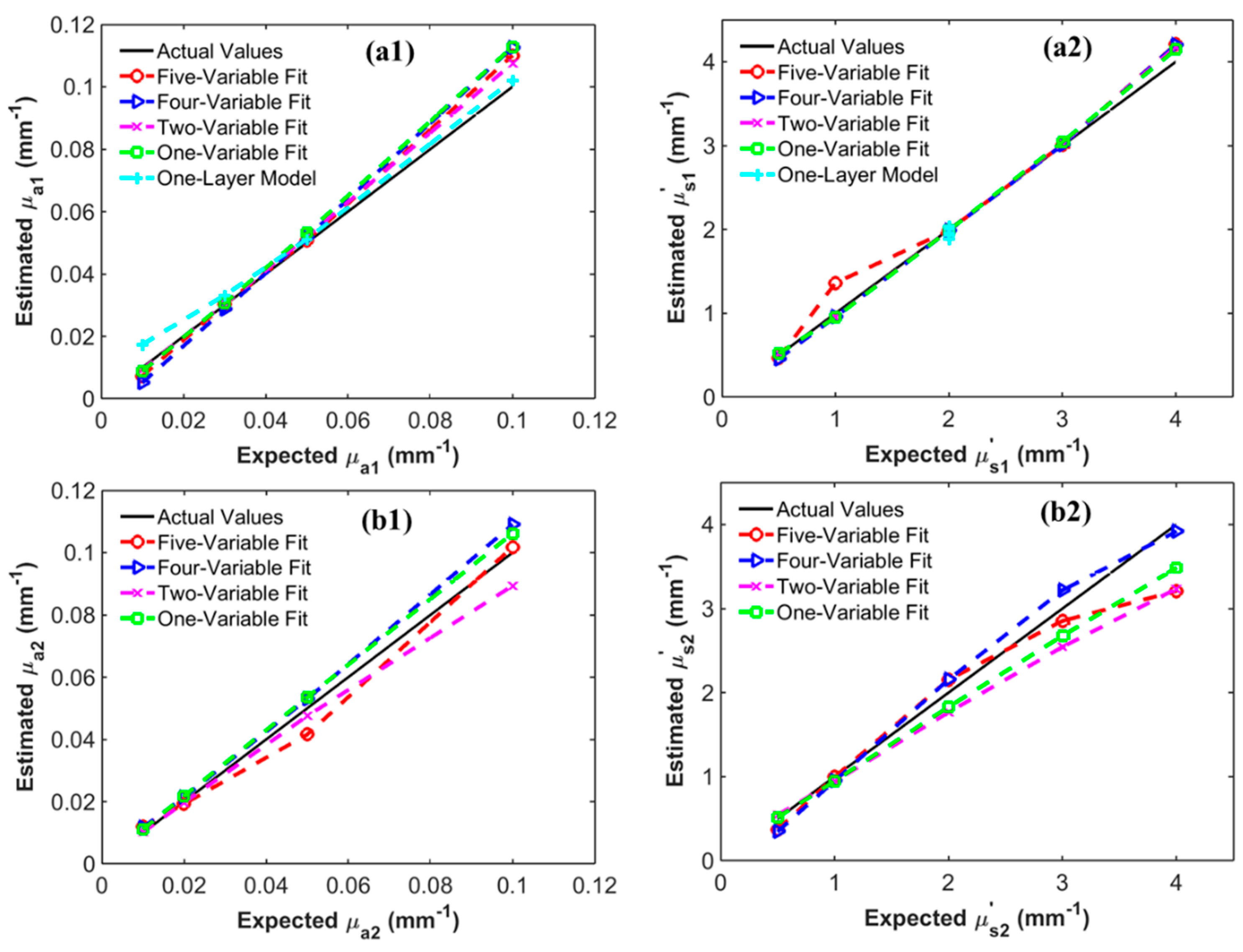
As mentioned in Section 2.3, the reflectance generated by MC simulation, after the correction, was much closer to that by the diffusion model, which was, therefore, used for optical property extraction in this study. Figure 3 shows estimated absorption and reduced scattering coefficients of each layer using different curve fitting methods. Note that the one-layered model was only used for estimating μa1 and μs1′ in Figure 3(a1,a2). The average absolute values of relative errors for the five curve fitting methods are summarized in Table 2. Overall, the accuracy for estimating μa1, μs1′, μa2 and μs2′ from the corrected reflectance are within 18%, which are superior to that without reflectance correction (results not presented here).
The accuracy for estimating μs1′ (Figure 3(a2)) was much better than that for μa1 (Figure 3a1) for all five curve fitting methods, which is consistent with the reflectance analyses in Section 3.1. It could be observed from Table 2 that five-variable fit performed the weakest for estimating μs1′, followed by the four-variable fit, confirming that estimation accuracy improves as fewer variables are to be estimated each time [5,7]. However, for estimating μa1, four-variable fit performed the weakest, followed by the one-layered model. These results are out of expectation that one-layered model with two unknown variables could obtain higher estimation accuracy than five- and four-variable fit methods. This may be partly explained by the fact that the light samples the bottom layer as well thus seeing in part its increased absorption, especially for lower μa1, while for high μa1, the detected light does no longer go through the bottom layer, making the one-layered model a well description. Moreover, the reflectance used for curve fitting was generated by MC simulation and corrected based on the values of μs1′ rather than μa1, which may also add challenges for estimating μa1 using the one-layered model; the value of μa1 is much smaller and more sensitive to the reflectance change than the μs1′. Detailed analyses show that the largest average error for estimating μa1 using one-layered model is caused by the first point where μa1 is equal to 0.01 mm−1 (shown in Figure 3a1).
For the bottom layer estimation in Figure 3(b1,b2)), estimation accuracy is much worse than for the top layer. Two- and one-variable fit improved the accuracy for estimating μa1, μs1′ and μa2, but the error values for estimating μs2′ using the two-variable fit were a little higher than the other three methods (Table 2). It is expected that the estimation accuracy of μa2 and μs2′ would be improved as the top-layer thickness decreases, because the detected light would carry more information related to the bottom layer.
In view of the fact that no a priori information about the optical properties of the bottom layer is available in practical applications, and after comparison of the average absolute errors for all five curve fitting methods, a stepwise method is suggested for estimating the optical properties of two-layered samples. First, μa1 and μs1′ are estimated using one-layered model. After obtaining μa1 and μs1′ estimations, the two-variable fit is used for estimating μa2 and μs2′, assuming that the top-layer thickness is known. It should be noted that one-layered model does not require a priori knowledge of the top-layer thickness for estimating μa1 and μs1′, compared to the other curve fitting methods (i.e., four-, two- and one-variable fit). The stepwise method reduces the number of constrained variables from five or four to two at every step, which could improve the overall estimation accuracy [12,13]. Therefore, the stepwise method was used for optical property estimations of two-layered samples going forward after Section 3.2 in this study.

3.3. Factors Influencing Optical Property Extraction of Top Layer

Accurate optical property extraction from the top layer is critical for the stepwise method because estimation results of the bottom layer are based on those from the top layer. Influencing factors of mfp1′/mfp2′, μa1/μa2 and μs1′/μs2′ determine the contributions of each layer on diffuse reflectance. Larger contribution implies higher accuracy for estimating the corresponding optical properties theoretically. Parameter of μs1′/μa1 is closely related to the assumption of diffusion model, which is the basis of Equation (1) and Equation (2) for optical property estimation. It is thus desirable to quantitatively evaluate the effects of the four factors. The results showed that factors of μa1/μa2 and μs1′/μs2′ had negligible effects on optical property extraction from the top layer (see Figures S1 and S2 in Supplementary Materials for more details). Hence only the factors of mfp1′/mfp2′ and μs1′/μa1 are discussed here, and the results are displayed in Figure 4 and Figure 5, respectively.
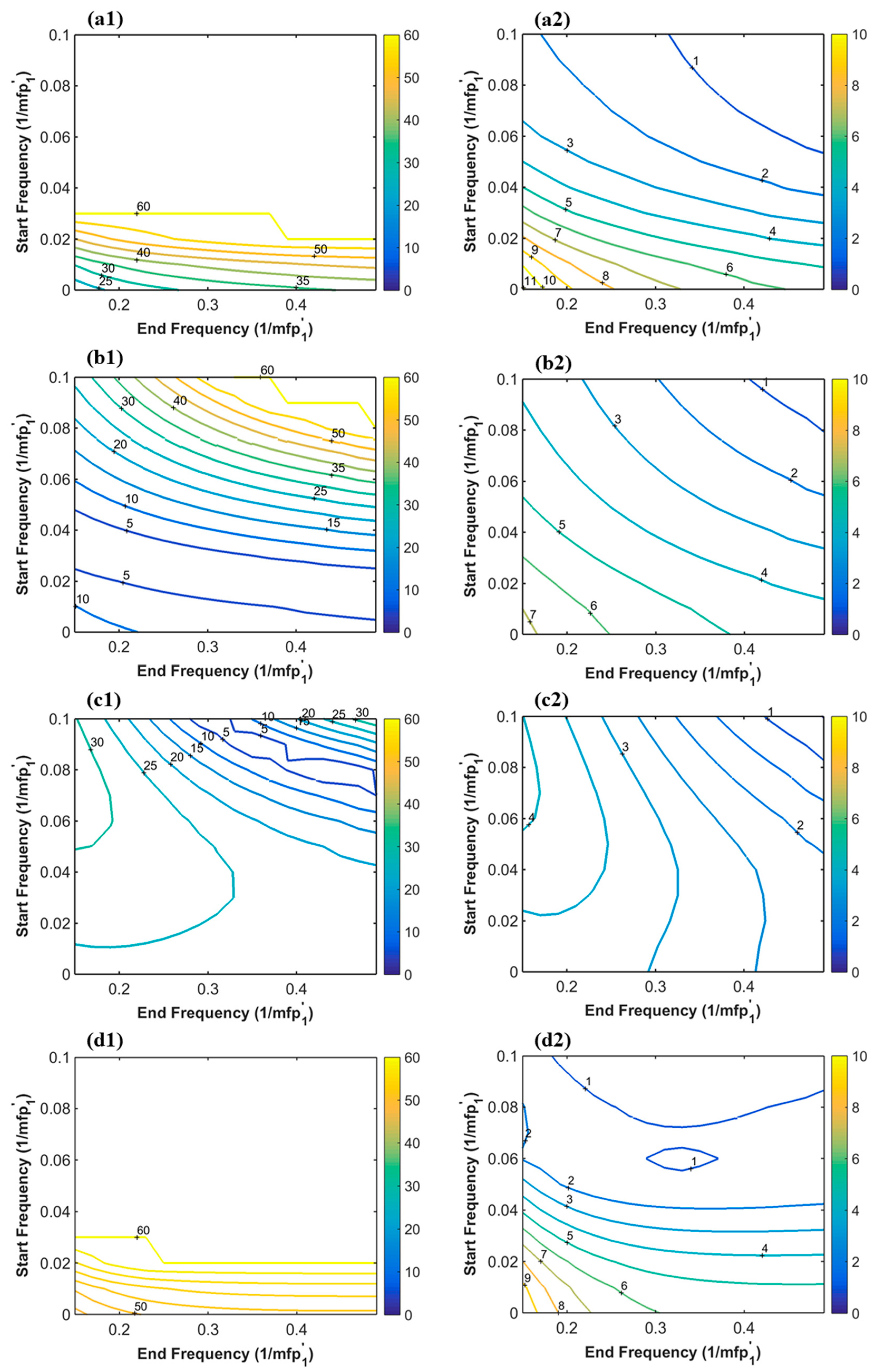
It is observed from Figure 4 that the absolute values of relative errors for estimating μa1 and μs1′ decreased first, and then increased with the increasing values of mfp1′/mfp2′. Further analysis showed that there were relatively small errors for μa1 and μs1′ when the values of mfp1′/mfp2′ were 1.2 and 1.6 (No. 26 and No. 27 in Table S2 of Supplementary Materials). This may be due to that the effective attenuation coefficients µeff of the bottom layer (1.36 and 1.57) and the top layer (1.60 and 1.60) are close to each other for both the two samples, resulting in similar light attenuation for the two layers. The absolute error contour maps also indicated that the optimal frequency region for estimating μs1′ was rather stable with relatively large start and end frequencies. This is because diffuse reflectance under large spatial frequency mainly depends on tissue scattering properties. For μa1, it is observed that the optimal start and end frequencies increased when the values of mfp1′/mfp2′ raised from 0.4 to 1.2 (Figure 4(a1,b1,c1)) due to the fact that larger mfp1′/mfp2′ lead to increased optical properties for the bottom layer, resulting in more effects on optical property estimations of the top layer. It was reported that structured illumination with larger frequencies resulted in shallower light interrogation [14,16,28], thus reducing and even eliminating the effects of the bottom layer on the estimation of μa1 and μs1′. These findings could provide references for optimizing frequency region for optical property estimations from the spatial-frequency domain reflectance.
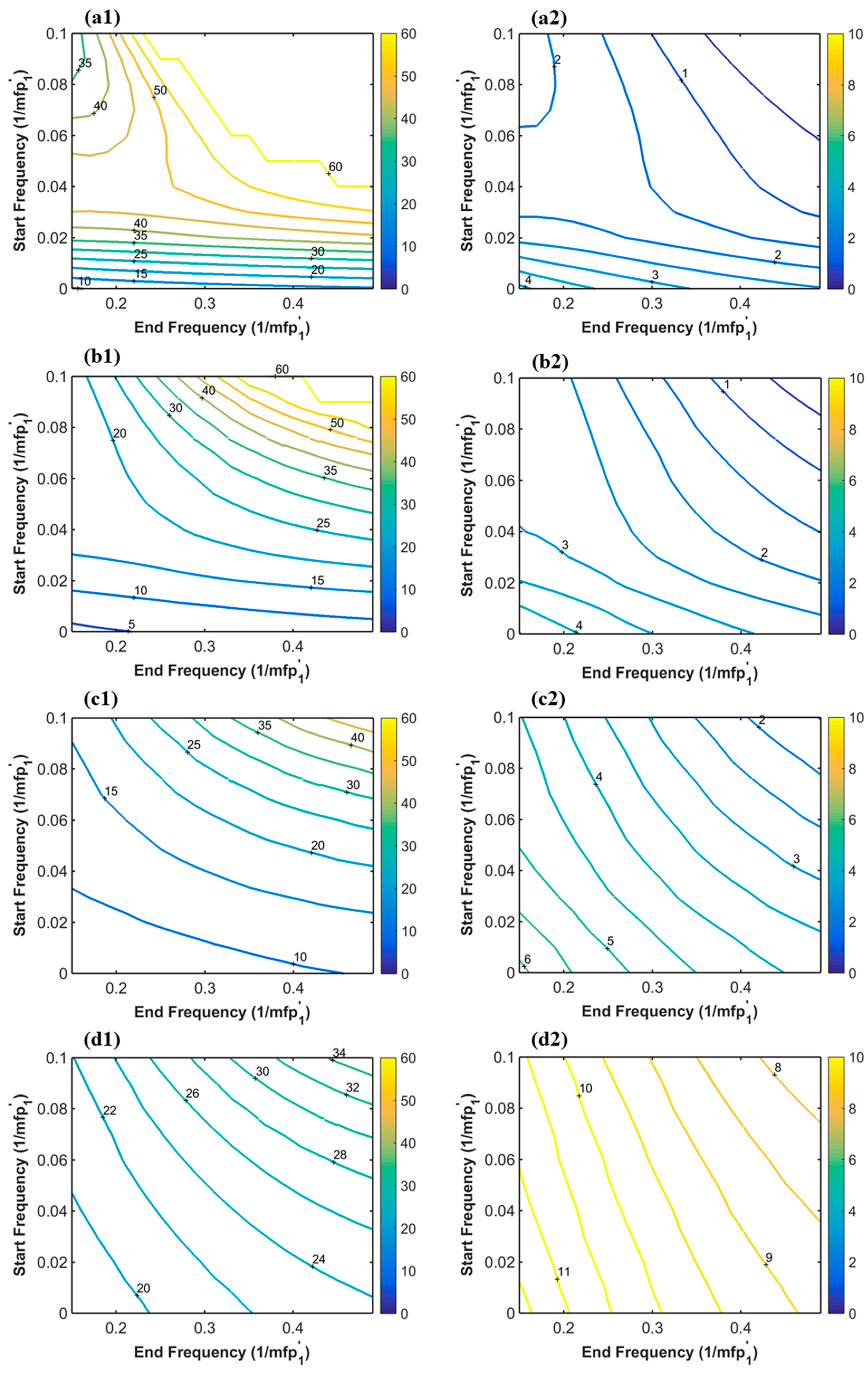
Figure 5 showed that the optimal frequency region for estimating both μa1 and μs1′ were relatively stable with varying values of μs1′/μa1. Absolute values of relative errors for estimating μs1′ increased with the decreased values of μs1′/μa1, which is in agreement with the expectation since the curve fitting is subject to the assumption of diffusion approximation (i.e., scattering dominant tissue). However, the error pattern for estimating μa1 did not obey this strictly. The absolute values of relative errors of μa1 reduced with the values of μs1′/μa1 decreasing from 133 to 20. Further analysis demonstrated that smaller μs1′/μa1 lead to larger values of μa1, which made μa1 be less sensitive to the variation and the parameter estimation for μa1 much easier (e.g., errors could reduce from 10 to 1% for μa1 values of 0.01 mm−1 and 0.1 mm−1, respectively, when the measured value deviated 0.001 mm−1 from the true value); even so, errors for estimating μa1 increased when the values of μs1′/μa1 were smaller than 10 (Figure 5(d1)), because too small μs1′/μa1 was beyond the boundary in which the optical properties could be estimated accurately from the diffusion model.
Overall, the discussion above suggests that the values of μs1′/μa1 should be no smaller than 10 to obtain accurate estimation of μa1 and μs1′ by using the stepwise method, which is applicable for most horticultural products due to the scattering-dominated property. Considering the findings that the optimal frequency region for estimating μa1 (that for μs1′ is relatively stable) varies with the values of mfp1′/mfp2′, it is strongly suggested to optimize the spatial frequency in terms of mfp1′ and/or mfp2′ for improving the estimation accuracy in future studies.

3.4. Relationship Between Light Penetration Depth and Spatial Frequency

Knowledge of light penetration depth is valuable because it could help us in optimizing the design of sensing configuration and parameter (i.e., illumination/detection geometry, sample presentation mode, detection angle, etc.) to collect effective information from the interior tissue of a target sample. Different methods have been proposed for measuring light penetration depth [29,30,31,32,33]. In diffuse optics, light penetration depth in horticultural products is typically defined as the travelling distance corresponding to a decay in power by a factor of 1/e (~37%). In the context of the steady-state diffuse approximation, light penetration depth of conventional uniform illumination depends on tissue optical properties (i.e., μa and μs′), which can be calculated using the following equation [34]:
δ = 1 μ e f f   = 1 3 μ a ( μ a + μ s )
where μeff is the effective attenuation coefficient. Under structured illumination of sinusoidal patterns in SFDI technique, the above equation can be modified as follows [16,35]:
δ = 1 μ e f f   = 1 μ e f f   2 + ( 2 π f x ) 2 + ( 2 π f y ) 2
where fx and fy are spatial frequencies along horizontal and vertical directions, respectively.
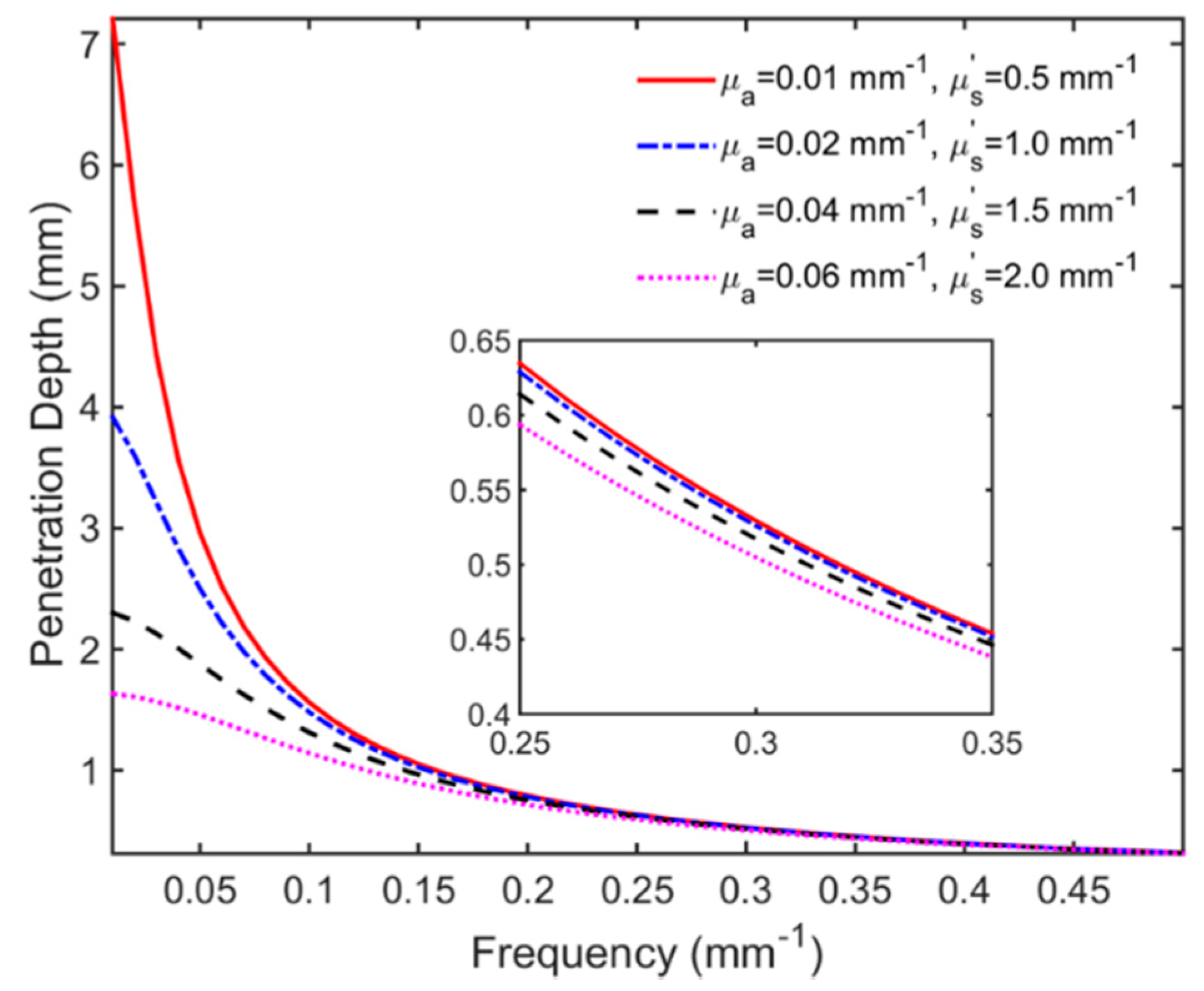
Equation (4) implies that light penetration depth under structured illumination depends, besides the tissue optical properties, on the spatial frequency of the sinusoidal patterns. High spatial frequency results in shallow penetration depth, which provides a theoretical guide for achieving the effective information in different depths by selecting appropriate spatial frequencies. Four sets of optical properties, which cover the common and typical range of horticultural products, were employed for studying the relationship between light penetration depth and spatial frequency, and the results are displayed in Figure 6. It could be observed that larger values of μa and μs′ generated shallower light penetration depth (pink dot line) since more light was absorbed or scattered while propagating within the tissues. This trend is especially true when the spatial frequency is smaller than 0.05 mm−1. According to this, the light penetration depth is estimated to be 0.5–5.5 mm for apple fruit with typical values of μa being 0.01–0.05 mm−1 and μs′ being 1.0–2.0 mm−1, respectively, in the wavelength region of 500–1000 nm. Note that the illumination pattern in this case is modulated only along the horizontal axis (i.e., fy = 0) with the spatial frequency fx varying from 0.01 to 0.3 mm−1.
In order to improve estimation accuracy for optical properties of two-layered horticultural products by using the stepwise method, it is suggested to have relatively large spatial frequency for estimating μa1 and μs1′ through one-layered model, and relatively small frequency for estimating μa2 and μs2′ through two-variable fit based on two-layered model. Effect of tissue optical properties on frequency selection should also be taken into account, which is consistent with the suggestions discussed in Section 3.3 (i.e., optimize the spatial frequency in terms of mfp1′ and/or mfp2′).

4. Discussion

Depth-varying characterization is the hallmark of SFDI technique under structured illumination with sinusoidal patterns, which is absent in conventional uniform illumination. However, the light penetration depth derived from Equation (4) does not always hold for actually detectable region for a general imaging system. In such cases, the light backscattered close to the illumination source contributes more to the detected signals, which correspond to a far more superficial depth of tissue interrogation than that derived from diffuse light attenuation. Moreover, due to the comprehensive consideration of imaging resolution, imaging contrast and signal-to-noise ratio, the factor of 1/e for light decaying in tissues is not always appropriate in practical applications, such as the subsurface bruise detection of fruit sample [36]. Since one goal of this study is to explore the potential of accuracy improvement for estimating optical properties of two-layered horticultural products by selecting appropriate frequency region, the relationship between light penetration depth and spatial frequency was just roughly investigated here. A more realistic experimental setting, such as three-dimensional modeling of the target sample with more layers [37], should be taken into account in the future for quantifying the light penetration depth, as well as the sampling volume (i.e., spatial distribution of detector depth sensitivity).
The cross effect of each layer is one of the challenging factors influencing optical property estimation of two-layered horticultural products. It is desirable to obtain the effective information of the target (top or bottom) layer when estimating the corresponding μa and μs′ without the interference of the other layer. The feature of depth-varying of SFDI provides a potential solution for solving this problem. The emitted optical signals under large spatial frequency carry more information related to the top layer, while those with relatively small spatial frequency penetrate deep into the bottom layer. It is thus possible to quantitatively select a spatial frequency, under which the captured signal is only related to the top layer. Then, an operation of subtraction between this signal and another one with smaller frequency can be used to eliminate the effect of the top layer. In principle, the signal after this operation should be more related to the bottom layer, and thus improving the estimation accuracy for μa and μs′ of the bottom layer. Take the apple fruit as a two-layered example with peel and flesh tissues. Subtraction operation for the demodulated reflectance between the small frequency and large frequency is expected to clear the peel information of apple sample, and the remaining reflectance will be more valuable for estimating μa and μs′ of the flesh tissue. It should be noted that this method may be limited for the two-layered horticultural products with relatively thin top-layer thickness (e.g., apple, peach and tomato) due to restricted light penetration depth (~1–2 mm) under the spatial frequency of 0.15 mm−1 [38]. The full potential of this method is worth exploring in the future research.
Thanks to the characteristics of the one-layered model, the stepwise method does not require a priori knowledge of the top-layer thickness for estimating μa1 and μs1′, but the top-layer thickness is still required to be known when estimating μa2 and μs2′ using the two-variable fit through the two-layered model. However, the top-layer thickness is usually unknown or difficult to be measured accurately, which brings challenges for optical property estimations of the bottom layer. Furthermore, the sample-based calibration method, which was employed for reflectance correction, may also bring some challenges when considering another optical property, i.e., the scattering phase function. Light backscattering at short source-detector separations is considerably influenced by the scattering phase function. In the spatial-frequency domain, as the horticultural product is illuminated by the structured lighting with high spatial frequency, part of the backscattered light would be referred to as sub-diffusive light, which largely depends on the scattering phase function. Different phase function parameters have been proposed for quantifying the influence of phase function on sub-diffusively backscattered light [39]. The influence of scattering phase function changed in the MC simulations on optical property estimations should be investigated.
In recent years, deep learning algorithms (e.g., generative adversarial networks, random forest, etc.) have evolved rapidly, which provide a means for accelerating and also improving optical property estimations of turbid materials [40,41,42]. What makes such methods attractive is their capacity to perform particularly well in learning nonlinear mappings. Unlike the conventional nonlinear curve fitting based on diffusion model, a deep learning method could predict optical properties directly from the SFDI images, without a priori knowledge of the top-layer properties (e.g., thickness, absorption and reduced scattering coefficients), which, however, require a sufficiently large image dataset to train the networks. Hence, future research efforts should also be directed at efficient utilization of deep learning for rapid and accurate optical property estimations of horticultural products.

5. Conclusions

This paper presents a theoretical analysis of intrinsic properties of the two-layered diffusion model and inverse algorithm through numerical simulation, including effect of optical parameter on reflectance prediction and optical property extraction, estimation accuracy of different curve fitting methods, and relationship between penetration depth and spatial frequency, in order to improve optical property estimation accuracy of two-layered horticultural products using SFDI technique. Reflectance prediction results indicated that there is good separation in diffuse reflectance over a large range of spatial frequencies for different μs1′ values, whereas less separation in diffuse reflectance for different μa1 values, and even less separation for different values of μa2 and μs2′, which is in agreement with accuracy for estimating optical properties. Evaluation of parameter estimation accuracy for all the five curve fitting strategies suggested to apply the stepwise method for estimating optical properties of two-layered samples, which estimated μa1 and μs1′ using the one-layered model first, followed with the estimation of μa2 and μs2′ using the two-variable fit. Investigation on the factors influencing the extraction of μa1 and μs1′, and relationship between penetration depth and spatial frequency offered great guidance for optimizing the frequency region for optical property estimation. Future work can be done on exploring the full potential of depth-varying features in SFDI for reducing or eliminating the effect of the top layer on estimating optical properties of the bottom layer.

Supplementary Materials

The following are available online at https://www.mdpi.com/2076-3417/11/2/617/s1, Figure S1: Absolute error contour maps for estimating μa1 (left panel) and μs1′ (right panel) of four representative two-layered simulation samples with varying values of μa1/μa2 by using the stepwise method with different start and end frequencies, Figure S2: Absolute error contour maps for estimating μa1 (left panel) and μs1′ (right panel) of four representative two-layered simulation samples with varying values of μs1′/μs2′ by using the stepwise method with different start and end frequencies, Table S1: Twenty two-layered simulation samples with different combinations of μa1, μs1′, μa2, μs2′and top-layer thickness d for investigating the effects of optical properties on reflectance prediction and comparing the estimation performance of diverse curve fitting methods, Table S2: Two-layered simulation samples with varying values of mfp1/mfp2′, Table S3: Two-layered simulation samples with varying values of μa1/μa2, Table S4: Two-layered simulation samples with varying values of μs1/μs2′, Table S5: Two-layered simulation samples with varying values of μs1/μa1.

Author Contributions

Conceptualization, D.H. and Y.H.; methodology, D.H. and T.S.; software, D.H.; validation, Y.H. and Q.Z.; writing—original draft preparation, D.H.; writing—review and editing, D.H., Y.H., Q.Z. and T.S.; supervision, L.Y. and Z.Y.; funding acquisition, D.H. All authors have read and agreed to the published version of the manuscript.

Funding

This research was funded by the Natural Science Foundation of Zhejiang Province (LQ20C130002), the Natural and Science Foundation of China (32001414), the Project of Key Laboratory in the Ministry of Agriculture and Rural Areas (2016NYZD18003) and the Startup Project of Zhejiang A&F University (2034020090).

Acknowledgments

The authors gratefully thank Renfu Lu in the U.S. Department of Agriculture Agricultural Research Service (USDA/ARS) for his great guidance and valuable advice.

Conflicts of Interest

The authors declare no conflict of interest.

References

  1. Huang, Y.; Lu, R.; Hu, D.; Chen, K. Quality assessment of tomato fruit by optical absorption and scattering properties. Postharvest Biol. Technol. 2018, 143, 78–85. [Google Scholar] [CrossRef]
  2. Sun, C.; Van Beers, R.; Aernouts, B.; Saeys, W. Bulk optical properties of citrus tissues and the relationship with quality properties. Postharvest Biol. Technol. 2020, 163, 111127. [Google Scholar] [CrossRef]
  3. Vanoli, M.; Van Beers, R.; Sadar, N.; Rizzolo, A.; Buccheri, M.; Grassi, M.; Lovati, F.; Nicolaï, B.; Aernouts, B.; Watté, R. Time-and spatially-resolved spectroscopy to determine the bulk optical properties of ‘Braeburn’apples after ripening in shelf life. Postharvest Biol. Technol. 2020, 168, 111233. [Google Scholar] [CrossRef]
  4. Kienle, A.; Patterson, M.S.; Dögnitz, N.; Bays, R.; Wagnières, G.; Van Den Bergh, H. Noninvasive determination of the optical properties of two-layered turbid media. Appl. Opt. 1998, 37, 779–791. [Google Scholar] [CrossRef] [PubMed]
  5. Cen, H.; Lu, R. Quantification of the optical properties of two-layer turbid materials using a hyperspectral imaging-based spatially-resolved technique. Appl. Opt. 2009, 48, 5612–5623. [Google Scholar] [CrossRef]
  6. Liemert, A.; Kienle, A. Analytical approach for solving the radiative transfer equation in two-dimensional layered media. J. Quant. Spectrosc. Radiat. Transf. 2012, 113, 559–564. [Google Scholar] [CrossRef]
  7. Wang, A.; Wei, X. A sequential method for estimating the optical properties of two-layer agro-products from spatially-resolved diffuse reflectance: Simulation. Artif. Intell. Agric. 2019, 3, 69–78. [Google Scholar] [CrossRef]
  8. Weber, J.R.; Cuccia, D.J.; Durkin, A.J.; Tromberg, B.J. Noncontact imaging of absorption and scattering in layered tissue using spatially modulated structured light. J. Appl. Phys. 2009, 105, 102028. [Google Scholar] [CrossRef] [Green Version]
  9. Tabassum, S.; Pera, V.; Greening, G.; Muldoon, T.J.; Roblyer, D. Two-layer inverse model for improved longitudinal preclinical tumor imaging in the spatial frequency domain. J. Biomed. Opt. 2018, 23, 076011. [Google Scholar] [CrossRef] [Green Version]
  10. Yudovsky, D.; Durkin, A.J. Spatial frequency domain spectroscopy of two layer media. J. Biomed. Opt. 2011, 16, 107005. [Google Scholar] [CrossRef]
  11. Yudovsky, D.; Nguyen, J.Q.M.; Durkin, A.J. In Vivo spatial frequency domain spectroscopy of two layer media. J. Biomed. Opt. 2012, 17, 107006. [Google Scholar] [CrossRef] [PubMed] [Green Version]
  12. Hu, D.; Lu, R.; Ying, Y. Spatial-frequency domain imaging coupled with frequency optimization for estimating optical properties of two-layered food and agricultural products. J. Food Eng. 2020, 277, 109909. [Google Scholar] [CrossRef]
  13. Hu, D.; Lu, R.; Ying, Y.; Fu, X. A stepwise method for estimating optical properties of two-layer turbid media from spatial-frequency domain reflectance. Opt. Express 2019, 27, 1124–1141. [Google Scholar] [CrossRef]
  14. Lu, Y.; Li, R.; Lu, R. Structured-illumination reflectance imaging (SIRI) for enhanced detection of fresh bruises in apples. Postharvest Biol. Technol. 2016, 117, 89–93. [Google Scholar] [CrossRef]
  15. Hu, D.; Fu, X.; He, X.; Ying, Y. Noncontact and wide-field characterization of the absorption and scattering properties of apple fruit using spatial-frequency domain imaging. Sci. Rep. 2016, 6, 37920. [Google Scholar] [CrossRef] [PubMed] [Green Version]
  16. Cuccia, D.J.; Bevilacqua, F.; Durkin, A.J.; Ayers, F.R.; Tromberg, B.J. Quantitation and mapping of tissue optical properties using modulated imaging. J. Biomed. Opt. 2009, 14, 024012. [Google Scholar] [CrossRef] [PubMed]
  17. Svaasand, L.O.; Spott, T.; Fishkin, J.B.; Pham, T.; Tromberg, B.J.; Berns, M.W. Reflectance measurements of layered media with diffuse photon-density waves. Phys. Med. Biol. 1999, 44, 801–813. [Google Scholar] [CrossRef] [Green Version]
  18. Hu, D.; Sun, T.; Yao, L.; Yang, Z.; Wang, A.; Ying, Y. Monte Carlo: A flexible and accurate technique for modeling light transport in food and agricultural products. Trends Food Sci. Technol. 2020, 102, 280–290. [Google Scholar] [CrossRef]
  19. Wang, L.; Jacques, S.L.; Zheng, L. MCML-Monte carlo modeling of photon transport in multi-layered tissues. Comput. Methods Programs Biomed. 1995, 47, 131–146. [Google Scholar] [CrossRef]
  20. Lu, R.; Van Beers, R.; Saeys, W.; Li, C.; Cen, H. Measurement of optical properties of fruits and vegetables: A review. Postharvest Biol. Technol. 2020, 159, 111003. [Google Scholar] [CrossRef]
  21. Xie, D.; Guo, W. Measurement and Calculation Methods on Absorption and Scattering Properties of Turbid Food in Vis/NIR Range. Food Bioprocess Technol. 2020, 13, 229–244. [Google Scholar] [CrossRef]
  22. Henyey, L.G.; Greenstein, J.L. Diffuse radiation in the galaxy. Astrophys. J. 1941, 93, 70–83. [Google Scholar] [CrossRef]
  23. Saeys, W.; Velazco-Roa, M.A.; Thennadil, S.N.; Ramon, H.; Nicolai, B.M. Optical propertie of apple skin and flesh in the wavelength range from 350 to 2200 nm. Appl. Opt. 2008, 47, 908–919. [Google Scholar] [CrossRef] [PubMed] [Green Version]
  24. Zhang, M.; Li, C.; Yang, F. Optical properties of blueberry flesh and skin and Monte Carlo multi-layered simulation of light interaction with fruit tissues. Postharvest Biol. Technol. 2019, 150, 28–41. [Google Scholar] [CrossRef]
  25. Sun, C.; Aernouts, B.; Van Beers, R.; Saeys, W. Simulation of light propagation in citrus fruit using monte carlo multi-layered (MCML) method. J. Food Eng. 2021, 291, 110225. [Google Scholar] [CrossRef]
  26. Aster, R.C.; Borchers, B.; Thurber, C.H. Parameter Estimation and Inverse Problems; Academic Press: Cambridge, MA, USA, 2011; Volume 90. [Google Scholar]
  27. Hu, D.; Lu, R.; Ying, Y. Finite element simulation of light transfer in turbid media under structured illumination. Appl. Opt. 2017, 56, 6035–6042. [Google Scholar] [CrossRef]
  28. Gigan, S. Optical microscopy aims deep. Nat. Photonics 2017, 11, 14–16. [Google Scholar] [CrossRef]
  29. Fraser, D.G.; Jordan, R.B.; Kunnemeyer, R.; McGlone, V.A. Light distribution inside mandarin fruit during internal quality assessment by NIR spectroscopy. Postharvest Biol. Technol. 2003, 27, 185–196. [Google Scholar] [CrossRef]
  30. Qin, J.; Lu, R. Monte Carlo simulation for quantification of light transport features in apples. Comput. Electron. Agric. 2009, 68, 44–51. [Google Scholar] [CrossRef]
  31. Wang, W.; Li, C. Measurement of the light absorption and scattering properties of onion skin and flesh at 633 nm. Postharvest Biol. Technol. 2013, 86, 494–501. [Google Scholar] [CrossRef] [Green Version]
  32. Chugunov, S.; Li, C. Monte Carlo simulation of light propagation in healthy and diseased onion bulbs with multiple layers. Comput. Electron. Agric. 2015, 117, 91–101. [Google Scholar] [CrossRef]
  33. Askoura, M.L.; Vaudelle, F.; L’Huillier, J.-P. Numerical study of light transport in apple models based on Monte Carlo simulations. Photonics 2016, 3, 2. [Google Scholar] [CrossRef] [Green Version]
  34. Tromberg, B.J.; Svaasand, L.O.; Tsay, T.-T.; Haskell, R.C. Properties of photon density waves in multiple-scattering media. Appl. Opt. 1993, 32, 607–616. [Google Scholar] [CrossRef] [PubMed] [Green Version]
  35. Cuccia, D.J.; Bevilacqua, F.; Durkin, A.J.; Tromberg, B.J. Modulated imaging quantitative analysis and tomography of turbid media in the spatial-frequency domain. Opt. Lett. 2005, 30, 1354–1356. [Google Scholar] [CrossRef]
  36. Lu, Y.; Li, R.; Lu, R. Gram-Schmidt orthonormalization for retrieval of amplitude images under sinusoidal patterns of illumination. Appl. Opt. 2016, 55, 6866–6873. [Google Scholar] [CrossRef]
  37. Meglinsky, I.; Matcher, S. Modelling the sampling volume for skin blood oxygenation measurements. Med. Biol. Eng. Comput. 2001, 39, 44–50. [Google Scholar] [CrossRef]
  38. Hayakawa, C.K.; Karrobi, K.; Pera, V.E.; Roblyer, D.M.; Venugopalan, V. Optical sampling depth in the spatial frequency domain. J. Biomed. Opt. 2018, 24, 071603. [Google Scholar] [CrossRef]
  39. Bodenschatz, N.; Krauter, P.; Liemert, A.; Kienle, A. Quantifying phase function influence in subdiffusively backscattered light. J. Biomed. Opt. 2016, 21, 035002. [Google Scholar] [CrossRef] [Green Version]
  40. Panigrahi, S.; Gioux, S. Machine learning approach for rapid and accurate estimation of optical properties using spatial frequency domain imaging. J. Biomed. Opt. 2018, 24, 071606. [Google Scholar] [CrossRef]
  41. Zhao, Y.; Deng, Y.; Bao, F.; Peterson, H.; Istfan, R.; Roblyer, D. Deep learning model for ultrafast multifrequency optical property extractions for spatial frequency domain imaging. Opt. Lett. 2018, 43, 5669–5672. [Google Scholar] [CrossRef]
  42. Chen, M.T.; Mahmood, F.; Sweer, J.A.; Durr, N.J. GANPOP: Generative Adversarial Network Prediction of Optical Properties from Single Snapshot Wide-field Images. IEEE Trans. Med. Imaging 2019, 39, 1988–1999. [Google Scholar] [CrossRef] [PubMed] [Green Version]
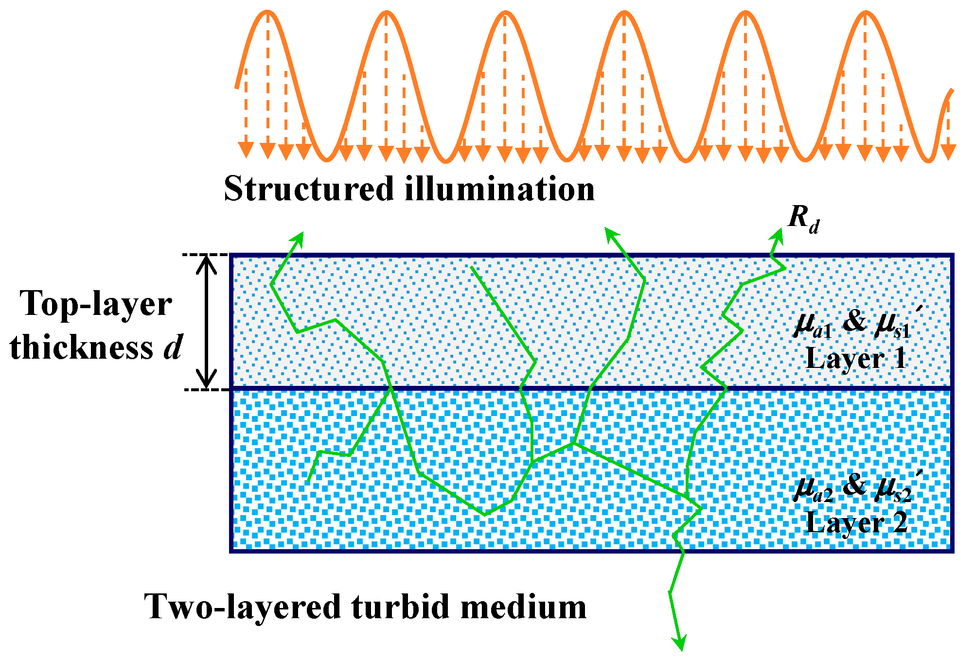
Figure 1. Schematic of a two-layered turbid medium under structured illumination. μa1, μa2, μs1′ and μs2′ are absorption and reduced scattering coefficients for the top layer and bottom layer, respectively, d is the thickness of the top layer, and Rd is the diffuse reflectance at the surface.
Applsci 11 00617 g001
Figure 2. Diffuse reflectance predicted by the two-layered diffusion model (Equation (2)) versus spatial frequency for varying optical properties in (a1) μa1 (μs1′ = 2 mm−1, μa2 = 0.02 mm−1, μs2′ = 1 mm−1 and d = 2 mm), (a2) μs1′ (μa1 = 0.03 mm−1, μa2 = 0.02 mm−1, μs2′ = 1 mm−1 and d = 2 mm), (b1) μa2 (μa1 = 0.03 mm−1, μs1′ = 2 mm−1, μs2′ = 1 mm−1 and d = 2 mm), and (b2) μs2′ (μa1 = 0.03 mm−1, μs1′ = 2 mm−1, μa2 = 0.02 mm−1 and d = 2 mm).
Applsci 11 00617 g002
Figure 3. Estimated absorption and reduced scattering coefficients of each layer from the corrected reflectance generated by Monte Carlo simulation using different curve fitting methods. (a1) μa1 varies 0.01–0.1 mm−1 with μs1′ = 2 mm−1, μa2 = 0.02 mm−1, μs2′ = 1 mm−1 and d = 2 mm, (a2) μs1′ varies 0.5–4 mm−1 with μa1 = 0.03 mm−1, μa2 = 0.02 mm−1, μs2′ = 1 mm−1 and d = 2 mm, (b1) μa2 varies 0.01–0.1 mm−1 with μa1 = 0.03 mm−1, μs1′ = 2 mm−1, μs2′ = 1 mm−1 and d = 2 mm, and (b2) μs2′ varies 0.5–4 mm−1 with μa1 = 0.03 mm−1, μs1′ = 2 mm−1, μa2 = 0.02 mm−1 and d = 2 mm.
Applsci 11 00617 g003
Figure 4. Absolute error contour maps for estimating μa1 (left panel) and μs1′ (right panel) of four representative two-layered simulation samples with varying values of mfp1′/mfp2′ by using the stepwise method with different start and end frequencies. The values of mfp1′/mfp2′ were 0.4, 0.8, 1.2 and 4 for (a), (b), (c) and (d), respectively. Different colors in the vertical bars on right of each graph denote different levels of error in percentage. Note that the absolute errors of μa1 and μs1′ larger than 60 and 20% were treated as 60 and 20% for better visual effect.
Applsci 11 00617 g004
Figure 5. Absolute error contour maps for estimating μa1 (left panel) and μs1′ (right panel) of four representative two-layered simulation samples with varying values of μs1′/μa1 by using the stepwise method with different start and end frequencies. The values of μs1′/μa1 were 133, 50, 20 and 5 for (a), (b), (c) and (d), respectively. Different colors in the vertical bars on right of each graph denote different levels of error in percentage. Note that the absolute errors of μa1 and μs1′ larger than 60 and 20% were treated as 60 and 20% for better visual effect.
Applsci 11 00617 g005
Figure 6. Relationship between light penetration depth and spatial frequency for a homogeneous sample under structured illumination of sinusoidal patterns with four sets of optical properties.
Applsci 11 00617 g006
Table 1. Different curve fitting methods for estimating optical properties of two-layered simulation samples.
Curve Fitting MethodEstimated ParameterKnown ParameterFitted Model
Five-variable fitμa1, μs1′, μa2, μs2′, d--Equation (2)
Four-variable fitμa1, μs1′, μa2, μs2dEquation (2)
Two-variable fitμa1, μs1′ or μa2, μs2′,the other threeEquation (2)
One-variable fitμa1 or μs1′ or μa2 or μs2the other fourEquation (2)
One-layered modelμa1, μs1--Equation (1)
Table 2. Average relative errors (in absolute values) of different curve fitting methods for estimating absorption (μa) and reduced scattering (μs′) coefficients of each layer.
Optical
Property
Five-Variable FitFour-Variable FitTwo-Variable FitOne-Variable FitOne-Layered Model
μa1 (%)9.8417.254.788.1412.23
μs1′ (%)9.813.722.772.902.66
μa2 (%)10.449.864.738.30--
μs2′ (%)11.6210.4812.118.15--
Publisher’s Note: MDPI stays neutral with regard to jurisdictional claims in published maps and institutional affiliations.