Abstract
Non-intrusive load monitoring (NILM) is a process of determining the operating states and the energy consumption of single electric devices using a single energy meter providing aggregate load measurements. Due to the large spread of power electronic-based and nonlinear devices connected to the network, the time signals of both voltage and current are typically non-sinusoidal. The effectiveness of a NILM algorithm strongly depends on determining a set of discriminative features. In this paper, voltage and current signals were combined to define, according to the definitions provided in Standard IEEE 1459, different power quantities, that can be used to distinguish different types of appliance. Multi-layer perceptron (MLP) classifiers were trained to solve the appliance detection problem as a multi-class event classification problem, varying the electric features in input. This allowed to select an optimal set of features guarantying good classification performance in identifying typical electric loads.
1. Introduction
Home energy management systems (HEMS) measure the energy consumption data of the household in real time for monitoring and optimizing the energy usage. Traditional intrusive monitoring systems collect fine-grained electricity data, posing higher initial cost for the homeowners since several smart meters must be plugged into the appliances. Non-intrusive load monitoring (NILM) systems allow to reduce hardware and maintenance costs since only one household-level smart meter is needed. As a consequence, the energy consumption at appliance-level is not available. NILM identifies a set of techniques that can disaggregate the power usage into the individual appliances that are functioning and disaggregate the consumption of electricity for each of them.
NILM has been an active area of research in the last years. One of the earliest studies about the NILM system was developed by Schweppe and Hart. In [1] the authors classify different appliances applying clustering algorithm in the active-reactive power features plane. Since the publication of this algorithm in 1992, the field of load-disaggregation has seen a tremendous amount of further research and novel approaches, see [2,3] for recent reviews. Furthermore, once the load has been disaggregated through a proper NILM technique, the disaggregated data can be used to improve the performance of some other important functionalities in the energy management system. This holds in particular for load demand forecasting [4], which may play a key role in the active management of modern distribution grid [3,5]. As an example, the method proposed in [6] first disaggregates the overall power into single appliances, so that the consumptions of each appliance can be forecasted separately, and then forecasts the total power of an aggregated set of houses by aggregating the single predicted powers. These NILM-based methods allow improving forecasting accuracy with respect to traditional methods that operate directly on the aggregate signal.
The most promising approaches recently presented in the literature for load disaggregation are based on machine learning techniques. A machine learning system classifies the switching events associating them to a particular appliance, processing significant features from the measured electrical parameters. Solutions based on machine learning range from classic supervised machine-learning algorithms (e.g., support vector machines, artificial neural networks, random forests) to supervised statistical learning methods (e.g., K-nearest neighbours and Bayes classifiers) and unsupervised method (e.g., hidden-Markov Models and its variants). Recently, deep learning (DL) methods were also employed and seem promising for the most challenging problem posed by the consumption profiles of multi-state appliances [7,8,9,10].
Commercial household smart meters usually provide the electric active and reactive power quantities measured at low frequency, typically on the order of a few values per second. As a consequence, these are the most widely used features and measurement rates reported in NILM-related literature. Since different appliances may show overlapping power values, performance is often unsatisfying. To overcome this issue, different features can be considered. Instantaneous samples acquired at high frequency (up to tens of kilohertz) have been proposed to extract information on the transient behavior of the supplied loads, but the drawbacks of these approaches are the increase in computational complexity and the real-time constraints associated with their implementation [3]. On the other hand, considering that the use of nonlinear appliances has increased continuously during the last decades, the frequency content of the involved electric signals can be exploited to improve the accuracy in the load identification process [11]. This implies the sampling rate used to acquired voltage and current signals must be sufficiently high to allow the frequency components of interest to be assessed correctly, but the measurement rate used in the disaggregation algorithm (i.e., the number of measured values per time unit, where each value is often obtained by processing a large number of instantaneous voltage and current samples), can be still in the order of few values per second, thus greatly improving the feasibility of these approaches with respect to the drawbacks mentioned above for the high-frequency solutions.
Based on these considerations, to take into account the presence of non-sinusoidal power draws, several authors recently resorted to additional information, extracting extremely detailed features such as, for example, V/I trajectory, harmonics of different orders [12], the harmonic phase [13,14], percentage total harmonic distortion (THD) [15], active and non-active current components [16], spectrograms of high-frequency current data [9]. The choice of the optimal set of features among them is crucial to maximize NILM effectiveness.
The literature contains few contributions where the different features were applied simultaneously. In [17] six different signal signatures have been applied such as current, current harmonics, real and reactive power, geometrical properties of the V–I curve and instantaneous power, for ten appliances.
Liang et al. [18] combine single-feature single-algorithm disaggregation methods, processing current waveform, active/reactive power, harmonics, instantaneous admittance waveform, instantaneous power waveform, eigenvalues, and switching transient waveform.
Gao et al. [19] apply real and reactive power, harmonics, quantized currents and voltages waveforms and V–I binary image obtaining better results with respect to those obtained with features belonging to one category.
In [20] the authors first explored a systematic approach of optimally combining features analyzing a plug load appliance identification dataset (PLAID) [21] retaining 58 features. Then, they performed several training sessions of the algorithm and the feature ranking and finally selected 20 features eliminating all of the voltage harmonics and all of the power-based features from transient state. The selected features included the total harmonic distortion (THD) of current, energy of detail wavelet coefficients at 2nd scale, enclosed area by V–I trajectory, current root mean square, 3-rd, 5-th, 9-th and 11-th current harmonic coefficient, THD of nonactive current and normalized real power.
In [22] the authors apply a complex hybrid energy disaggregation approach and propose a monitoring system consisting of a composite dual sliding window-based cumulative sum control chart (DSWC) to detect the transient event, a multi-layer Hungarian matching process to match load events. The detected events are converted to a bipartite graph optimization; a supervised clustering procedure is used to activate the corresponding category. Input data consist of rms current and voltage, active power, reactive power and the 15-th harmonic of the current.
This paper focuses on the choice of a suitable set of features for a non-intrusive load monitoring system, providing the following main contributions:
- different power terms, accounting for possible distortion in the voltage and current signals, have been considered as possible features;
- the power terms have been evaluated in different time intervals after the detected event;
- a systematic approach to rapidly obtain the lowest possible number of features preserving model performance has been explored applying two procedures of feature selection.
The most effective feature sets are given as input to a multi-layer perceptron (MLP) classifier trained to identify the on/off events for each device. The procedure is applied to Building-Level fUlly-labeled for Electricity Disaggregation (BLUED) dataset [23]. BLUED is a big dataset consisting of real voltage and current measurements for a single-family residence in the United States, sampled at 12 kHz for a whole week. BLUED is publicly available and it has been applied as benchmark dataset in several recent papers on NILM [22,24].
2. Feature Definition
Nowadays, due to the large spread of power electronic-based and nonlinear devices connected to the network, the time signals of both voltage and current, respectively v(t) and i(t), are typically non-sinusoidal. In particular, for steady state conditions, these signals can be modelled by considering two components:
- the fundamental component, typically denoted with the subscript 1, that is a sinusoidal signal at system frequency f1:where , while , and I1, β1, are the root mean square (rms) and the initial phase angle for voltage and current, respectively
- the remaining term, typically denoted with the subscript H, which is obtained by summing up the sinusoids of all the harmonics and the possible dc component.where , , , and are the rms and the initial phase angle of the voltage and current h-th order harmonic component.
Consequently, the time signals of both voltage and currents can be obtained as follows:
With reference to the analysis of a single-phase system, and according to the standard IEEE 1459 [25], it is possible to combine the two components of both voltage and current signals to define a number of different rms and power quantities. Among all the quantities proposed in the standard [25], the focus of this work will be on the 4 power-based quantities shown in Table 1, where is the phase displacement between the h-th harmonic components of voltage and current. Parameters related to voltage were excluded because voltage variations are minimal while connecting and disconnecting loads mainly affect the current draws and power consumptions.

Table 1.
Definitions of the considered power quantities under non-sinusoidal conditions, according to [25].
According to their definitions, the power terms shown in Table 1 include information on the fundamental components (namely active, fundamental active and fundamental reactive power) and on the harmonic components (namely harmonic active power). These quantities will be considered as possible features in the proposed NILM approach and will be referred to as parameters in the following, for the sake of brevity. In the following, the variation of all the parameters due to an event will be used as possible source of information to determine which load caused the event.
3. Database Creation
When testing the performance of a NILM technique, it is important to consider real data. Due to the challenges in the creation of such data sets, mainly related to the required time and the high costs involved, researchers typically refer to data sets that have been shared online and can be used as common reference. This choice also allows comparing the performance of different approaches.
3.1. BLUED
Among all the datasets available in literature, in this work the BLUED dataset [23] has been considered. This dataset was built in 2011 by monitoring a whole house located in Pennsylvania (USA), for 8 days. It contains the samples of voltage and current signals, and the corresponding timestamps, collected with a sampling frequency of . During the creation of the data set, all the changes in the state of power consumption higher than 30 W and lasting at least 5 s, for almost 50 appliances, have been labelled and recorded. This results in 2355 events recorded from known sources, and additional 127 events recorded from unknown sources, for a total of 2482 events. In this work, only the events involving appliances with a nominal active power higher than 30 W, with more than 10 recorded events, have been considered, resulting in 1585 events. In Table 2, the list of the considered appliances is reported, together with the identification code in the BLUED dataset (appliance label), and the number of recorded events.
Table 2.
Lists of the considered appliances from BLUED dataset.
3.2. Signal Processing
In order to be able to evaluate all the electrical quantities in Table 1, the time signals stored in the BLUED database have been processed through a standard scheme, described in the following.
Before to proceed with the evaluation of the electrical quantities of interest, according to a generic timeline such as the one represented in Figure 1, it is important to focus on a specific section of both voltage and current signals. Given , the time instant in which an event occurs for the generic device, a 2 s time window, centered in , is selected. Consequently, the selected portion of the signal is divided in 8 observation windows (), each one 15 cycles long (250 ms at the 60 Hz rated frequency).
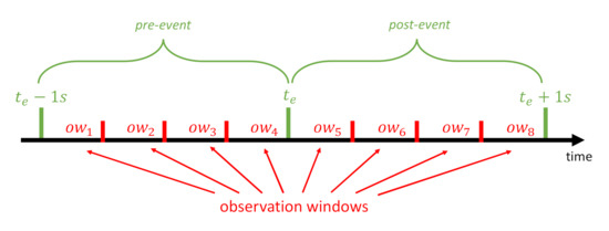
Figure 1.
Representation of a generic timeline.
For each observation window, a calculation window is selected, by considering 10 cycles starting from the first zero-crossing in the voltage signal. Then, the fast Fourier transform (FFT) is applied to each calculation window of both voltage and current signals. In particular, since the bandwidth of the acquisition system for the BLUED database was limited to 300 Hz, only the frequency components up to the 5th order have been considered to evaluate all four electric parameters by means of Equations (7)–(10). This results in eight values for each one of the four parameters: four values for the pre-event period and four values for the post-event period, stored in a matrix :
In order to define a reference value representative of the pre-event scenario for the k-th parameter, the mean value among the four pre-event values has been considered:
The obtained reference values have been then considered to evaluate the variation of the -th parameter due to the occurrence of the event, , according to the following equation:
where, given , the superscript denotes the index of the post-event values of the parameter . Consequently, the matrix containing the variations of all the parameters, named , has been obtained:
Then, these values have been used to train and test the neural network in charge of the identification of the device that caused the event. The time instants corresponding to the ON/OFF events are considered known.
4. The Multilayer Perceptron
Multilayer perceptrons (MLPs) are feedforward artificial neural networks consisting of at least three layers of nodes called input layer, hidden layer and output layer.
The relationship between input and output patterns is described by the following algebraic equations system:
where is the input vector, is the weights matrix of the input layer, is the bias vector of the input layer, is the input of the hidden layer, is the output of the hidden layer, is the hidden neurons nonlinear activation function, is the weights matrix of the output layer, is the bias vector of the output layer, o is the output vector. Feedforward networks can be trained for classification purposes, i.e., to classify input data according to the specified target classes.
Learning occurs through a supervised learning procedure, by evaluating the error in the neural network output after each input pattern is fed to the network and modifying the connection weights, in order to minimize the error. In this case the conjugate gradient algorithm is applied to train any network [26] and the error function to be minimized with respect to the weight and bias variables is the cross entropy. For each pair of output class/target class the cross-entropy is calculated as:
The cross entropy penalizes the classification errors in the different classes, mainly penalizing misclassifications that are confident. The aggregate cross-entropy performance is the mean of the individual values.
Figure 2 shows the structure of the MLP neural network considered in this paper. The variables used as input are the selected features, whereas the output of the network consists of a binary vector in which the neuron corresponding to the ON or OFF event of an appliance is set equal to 1. Hence, the dimension of the output vector is twice the number of the considered appliances (44 in the case study).
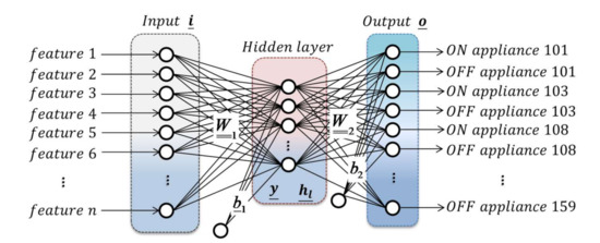
Figure 2.
The MLP architecture.
In order to obtain an unbiased evaluation of the neural model fit, the available dataset is generally split into three sets. The Training set is used to fit the model and determine weights and biases; the Validation set is used for parameter selection and it should provide an unbiased evaluation of the fit during the network training. During training, the error of each model is checked on the validation set and the model that achieves the lowest validation error is selected. This is the final choice of features and model. The Test set is used once the training is completed to evaluate the performance of the final model.
5. Feature Selection
Feature selection is the procedure performed to reduce the number of input variables when developing a model in order to facilitate the learning and the interpretation, reduce the computational cost and often improve the model performance. The addition of unrelated or redundant features influences model accuracy: redundant features increase the model complexity enhancing the risk of overfitting. Moreover, they could introduce spurious correlations between the features and the class labels.
Many feature extraction algorithms map the parameters in a lower dimensional feature space, suffering from the lack of interpretation of the projection dimensions. In this case, the two methods chosen in this work retain a subset of original features allowing further interpretation of physical meaning behind the selection.
The first method is based on neighborhood component analysis (NCA) [27], which implements a feature weighting approach to optimize the nearest neighbor classifier performance by maximizing an objective function that evaluates the average leave-one-out classification accuracy over the training data. However, the cost function of NCA is prone to overfitting, and an improved version of NCA with a regularization term was proposed by Yang et al. [28], where the regularization term was selected empirically.
In the second method, the ranking is done applying minimum redundancy maximum relevance (MRMR) algorithm. The MRMR algorithm [29] minimizes the redundancy of a feature set while maximizing the relevance of the feature set to the target. Redundancy and relevance are expresses by the mutual information of features and mutual information of a feature and the target.
It is worth noting that there is no guarantee that the feature selection algorithm will supply a feature ranking applicable to a generic classifier, based on a different algorithm. However, in practice, the significance of features can often be generalized, especially when both algorithms show good performance in classification. The outcome of the feature ranking was used to design a set of tests employing an increasing number of features.
6. Performance Indexes
The results have been evaluated using the metric F-score, which is defined as:
Precision is the ratio between the number of correctly detected appliances (true positive (TP)) and the total number of the detected ones (TP + false positive (FP)), and it represents the fraction of correct detections.
The recall is the ratio between the number of correctly detected appliances (TP) and the total number of appliances in the dataset (TP + false negative (FN)) and it represents the fraction of events that has been detected.
The confusion matrix is useful for visualizing precision and recall for the different classes. A confusion matrix for multiclass classification shows the different classifier answers. The actual values form the columns, and the predicted values form the rows. The intersection of the rows and columns show one of the answers.
7. Test and Results
To obtain the results, data where split in three parts. For each appliance, the 80% of events is used for training, the 10% for validation and the other 10% for test. On this training set, cross-validation was applied in order to avoid overfitting. From the cross-validation results, optimal configuration settings for the methods were obtained and the evaluation on the test set gave us the final performance. The composition of the three datasets is reported in Table 3.
Table 3.
Training, Validation and Test sets composition.
7.1. Feature Selection
Figure 3a,b report the cumulative feature weights (CFW) obtained applying the NCA and MRMR methods to the training set respectively, cumulating from the most important to the less one.
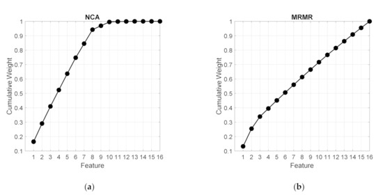
Figure 3.
Cumulative Feature Weights for training data (a) NCA algorithm (b) MRMR algorithm.
As it can be noticed, the CFW curve for NCA algorithm shows a clear linear growth for the top eight features of the ranking and saturation after a knot point. As shown in Figure 4, these features include active power, fundamental active and reactive power for the 3rd and 4th time instant after the event; and harmonic active power in the 2nd and 4th time instant after the event. Thus, also the dynamic of these parameters supplies useful information, since in some cases the same parameter is selected in different time instants. In order to detect the relevant features, the best regularization parameter that corresponds to the minimum average loss has been obtained using cross-validation. In Figure 5 the average loss values versus the regularization parameter values obtained with this optimization procedure is shown.
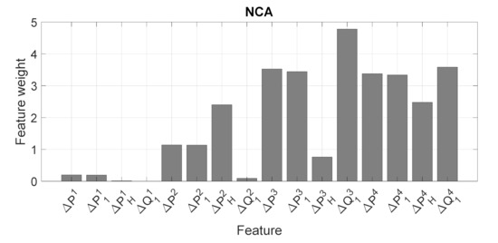
Figure 4.
The feature weights obtained with the NCA algorithm. The weights of the irrelevant features are very close to zero. The superscript identifies the observation window after the event.
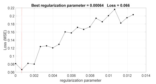
Figure 5.
The average loss values versus the regularization parameter for the NCA algorithm.
The feature score proposed by MRMR algorithm does not suggest any cut on the feature ranking since the CFW curve continues to linearly grow until the bottom feature is added. Thus, no useful information is supplied by the algorithm in this context.
7.2. Load Classification Results
Following the NCA suggestion, for each number of features, a bunch of training sessions was done varying the number of hidden neurons from 10 to 100 for an MLP, choosing as input the 8 top features.
Results are reported in Table 4 for the network with 50 hidden neurons showing the best validation error. Figure 6 shows the confusion matrix. Since training, validation and test sets show similar performance, the confusion matrix is built for the entire dataset.
Table 4.
Performance of MLP trained with the top 8 features.
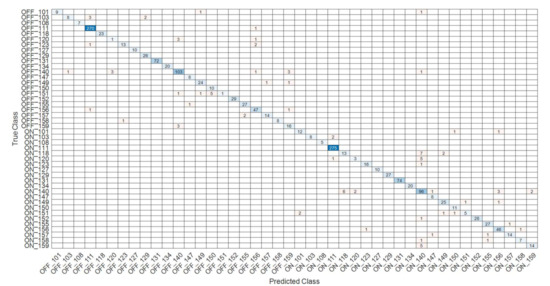
Figure 6.
Confusion matrix for the entire dataset.
In order to verify the goodness of the approach, the MLP classifier was trained varying the number of hidden neurons from 10 to 100. The network with 50 hidden neurons shows the minimum validation error, so it has been assumed as the best model.
Figure 7 shows the performance in term of cross-entropy obtained by progressively entering the input features following the ranking provided by NCA algorithm. As it can be noticed, increasing the number of features initially improves model performance. The major improvement is obtained adding the fundamental active power. Then, the validation error fairly decreases, and best results are obtained when 8 features are selected. Further increasing the input dimension does not provide more accurate classifications. Thus, the test confirms the goodness of the choice suggested by the NCA algorithm.
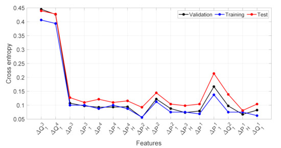
Figure 7.
Training, Validation and Test sets error for different number of input features. The horizontal axis shows the features added to the MLP input for each training session. The superscript identifies the observation window after the event.
The model performance was compared with those shown when the MLP is fed with the fundamental active and reactive power ΔP1 and ΔQ1, widely applied in literature, also by the authors [30,31], and adding to them the harmonic power that includes the information on the non-sinusoidal current.
Table 5 reports the results for the described tests.
Table 5.
Training, Validation and Test sets performance for additional tests.
Although the obtained performances are slightly worse than those achieved by the NMR top features, results confirm that relevant information is carried out by the fundamental and harmonic active power features in different time instants.
Performance evaluation and comparison of different approaches to NILM remain open issues in literature because the authors test their techniques on different datasets, with different criteria and metrics. In this paper, in order to make a meaningful comparison, the techniques proposed in [22,24] and [9] have been considered. In all three cases BLUED dataset is used and the performance is evaluated with the same indices considered in the present paper.
In particular, in [22] the authors apply a complex multivariable hybrid energy disaggregation approach to a subset of BLUED database consisting of 24 h of monitoring. The study is limited to the following six devices: fridge, air compressor, hair dryer, backyards lights, bathroom upstairs light, bedroom lights for 107 events, obtaining a F-score equal to 91.8%. Table 6 reports the obtained performance for five individual appliances both for [22] and the present paper.
Table 6.
Comparison with the performance reported in [22] for five appliances of BLUED.
In [24] random forest algorithms are applied to active and reactive powers for the devices in BLUED dataset. The performance for the load classification step is reported in Table 7.
Table 7.
Performance reported in [24] for random forest algorithms applied to BLUED dataset.
In [9] the authors apply a deep neural network, called concatenate convolutional neural network, to high-dimensional spectrograms of high-frequency current data. Data are a subset of BLUED database (537 samples) sampled to 2 kHz and the devices are grouped in six classes: fridge, two groups of lights, two groups of high-power devices and one group with computer and monitor. Table 8 reports the classification performance.
Table 8.
Performance reported in [9] for concatenate convolutional neural networks applied to six classes of devices in BLUED dataset.
Even if all these results are not directly comparable since the datasets, although selected from BLUED data, are different in composition and size, they confirm the goodness of the proposed approach for the appliance classification.
8. Conclusions
This study presents the effectiveness of NCA as a feature selection method to enhance the classification performance of a multilayer perceptron for non-intrusive load monitoring. Two feature selection methods, namely the neighborhood component analysis and minimum redundancy maximum relevance algorithms, have been applied to a set of sixteen features including active fundamental and harmonic active power and fundamental reactive power in four windows successive to a switching event. The results reveal that NCA feature selection method can select an optimal set of features tackling the model complexity. Indeed, the top features of the algorithm, fundamental active and reactive power and active power harmonics, allows one to obtain the best MLP performance also reducing the model complexity. Comparisons with results presented in literature show that the procedure achieves competitive performance despite the model simplicity.
Author Contributions
Conceptualization, B.C., S.C., D.C. and C.M.; methodology, B.C., S.C., D.C. and C.M.; software, S.C. and D.C.; validation, B.C., S.C. and D.C.; formal analysis, B.C. and S.C.; investigation, B.C., S.C. and D.C.; resources, S.C. and D.C.; data curation, S.C. and D.C.; writing—original draft preparation, S.C. and D.C.; writing—review and editing, B.C., S.C., D.C. and C.M.; visualization, B.C. and S.C.; supervision, B.C., C.M. and A.F.; project administration, C.M.; funding acquisition, C.M. and B.C. All authors have read and agreed to the published version of the manuscript.
Funding
This research was funded by Sardinian Region under project “RT-NILM (Real-Time Non-Intrusive Load Monitoring for intelligent management of electrical loads)”, Call for basic research projects, year 2017, FSC 2014–2020.
Institutional Review Board Statement
Not applicable.
Informed Consent Statement
Not applicable.
Data Availability Statement
The data presented in this study are available on request from the corresponding author.
Conflicts of Interest
The authors declare no conflict of interest. The funders had no role in the design of the study, in the collection, analyses, or interpretation of data; in the writing of the manuscript, or in the decision to publish the results.
References
- Hart, G.W. Nonintrusive Appliance Load Monitoring. Proc. IEEE 1992, 80, 1870–1891. [Google Scholar] [CrossRef]
- Hosseini, S.; Agbossou, K.; Kelouwani, S.; Cardenas, A. Non-Intrusive Load Monitoring through Home Energy Management Systems: A Comprehensive Review. Renew. Sustain. Energy Rev. 2017, 79, 1266–1274. [Google Scholar] [CrossRef]
- Ruano, A.E.; Hernández, Á.; Ureña, J.; Ruano, M.G.; Garcia, J. NILM Techniques for Intelligent Home Energy Management and Ambient Assisted Living: A Review. Energies 2019, 12, 2203. [Google Scholar] [CrossRef]
- Hong, W.-C.; Li, M.-W.; Fan, G.-F. Short-Term Load Forecasting by Artificial Intelligent Technologies; MDPI: Basel, Switzerland, 2019. [Google Scholar]
- Welikala, S.; Dinesh, C.; Ekanayake, M.P.B.; Godaliyadda, R.I.; Ekanayake, J. Incorporating Appliance Usage Patterns for Non-Intrusive Load Monitoring and Load Forecasting. IEEE Trans. Smart Grid 2019, 10, 448–461. [Google Scholar] [CrossRef]
- Dinesh, C.; Makonin, S.; Bajić, I.V. Residential Power Forecasting Using Load Identification and Graph Spectral Clustering. IEEE Trans. Circuits Syst. II Express Briefs 2019, 66, 1900–1904. [Google Scholar] [CrossRef]
- Kong, W.; Dong, Z.; Wang, B.; Zhao, J.; Huang, J. A Practical Solution for Non-Intrusive Type II Load Monitoring Based on Deep Learning and Post-Processing. IEEE Trans. Smart Grid 2020, 11, 148–160. [Google Scholar] [CrossRef]
- Harell, A.; Makonin, S.; Bajic, I. Wavenilm: A Causal Neural Network for Power Disaggregation from the Complex Power Signal. In Proceedings of the ICASSP 2019–2019 IEEE International Conference on Acoustics, Speech and Signal Processing (ICASSP), Brighton, UK, 12–17 May 2019; pp. 8335–8339. [Google Scholar] [CrossRef]
- Wu, Q.; Wang, F. Concatenate Convolutional Neural Networks for Non-Intrusive Load Monitoring across Complex Background. Energies 2019, 12, 1572. [Google Scholar] [CrossRef]
- Davies, P.; Dennis, J.; Hansom, J.; Martin, W.; Stankevicius, A.; Ward, L. Deep Neural Networks for Appliance Transient Classification. In Proceedings of the ICASSP 2019-2019 IEEE International Conference on Acoustics, Speech and Signal Processing (ICASSP), Brighton, UK, 12–17 May 2019; pp. 8320–8324. [Google Scholar] [CrossRef]
- Bucci, G.; Ciancetta, F.; Fiorucci, E.; Mari, S. Load Identification System for Residential Applications Based on the NILM Technique. In Proceedings of the 2020 IEEE International Instrumentation and Measurement Technology Conference (I2MTC), Dubrovnik, Croatia, 25–28 May 2020; pp. 1–6. [Google Scholar]
- Djordjevič, S.; Simic, M. Nonintrusive Identification of Residential Appliances Using Harmonic Analysis. Turk. J. Electr. Eng. Comput. Sci. 2018, 26, 780–791. [Google Scholar] [CrossRef]
- Djordjevič, S.; Dimitrijević, M.; Litovski, V. A Non-Intruive Identification of Home Appliances Using Active Power and Harmonic Current. FACTA Univ. Electron. Energ. 2017, 30. [Google Scholar] [CrossRef]
- Shi, X.; Ming, H.; Shakkottai, S.; Xie, L.; Yao, J. Nonintrusive Load Monitoring in Residential Households with Low-Resolution Data. Appl. Energy 2019, 252, 113283. [Google Scholar] [CrossRef]
- Devarapalli, H.P.; Dhanikonda, V.S.S.S.S.; Gunturi, S.B. Non-Intrusive Identification of Load Patterns in Smart Homes Using Percentage Total Harmonic Distortion. Energies 2020, 13, 4628. [Google Scholar] [CrossRef]
- Faustine, A.; Pereira, L. Multi-Label Learning for Appliance Recognition in NILM Using Fryze-Current Decomposition and Convolutional Neural Network. Energies 2020, 13, 4154. [Google Scholar] [CrossRef]
- Lin, S.; Zhao, L.; Li, F.; Liu, Q.; Li, D.; Fu, Y. A Nonintrusive Load Identification Method for Residential Applications Based on Quadratic Programming. Electr. Power Syst. Res. 2016, 133, 241–248. [Google Scholar] [CrossRef]
- Liang, J.; Ng, S.K.K.; Kendall, G.; Cheng, J.W.M. Load Signature Study—Part I: Basic Concept, Structure, and Methodology. IEEE Trans. Power Deliv. 2010, 25, 551–560. [Google Scholar] [CrossRef]
- Gao, J.; Kara, E.C.; Giri, S.; Bergés, M. A Feasibility Study of Automated Plug-Load Identification from High-Frequency Measurements. In Proceedings of the 2015 IEEE Global Conference on Signal and Information Processing (GlobalSIP), Orlando, FL, USA, 14–16 December 2015; pp. 220–224. [Google Scholar]
- Sadeghianpourhamami, N.; Ruyssinck, J.; Deschrijver, D.; Dhaene, T.; Develder, C. Comprehensive Feature Selection for Appliance Classification in NILM. Energy Build. 2017, 151, 98–106. [Google Scholar] [CrossRef]
- Gao, J.; Giri, S.; Kara, E.C.; Bergés, M. PLAID: A Public Dataset of High-Resoultion Electrical Appliance Measurements for Load Identification Research: Demo Abstract. In Proceedings of the 1st ACM Conference on Embedded Systems for Energy-Efficient Buildings, Memphis, TN, USA, 4–6 November 2014; Association for Computing Machinery: New York, NY, USA, 2014; pp. 198–199. [Google Scholar]
- Liu, H.; Zou, Q.; Zhang, Z. Energy Disaggregation of Appliances Consumptions Using HAM Approach. IEEE Access 2019, 7, 185977–185990. [Google Scholar] [CrossRef]
- Anderson, K.; Ocneanu, A.; Benitez, D.; Carlson, D.; Rowe, A.; Berges, M. BLUED: A Fully Labeled Public Dataset for Event-Based Non-Intrusive Load Monitoring Research. In Proceedings of the 2nd KDD workshop on data mining applications in sustainability (SustKDD), Beijing, China, 12–16 August 2012; pp. 1–5. [Google Scholar]
- Taveira, P.R.Z.; Moraes, C.H.V.D.; Lambert-Torres, G. Non-Intrusive Identification of Loads by Random Forest and Fireworks Optimization. IEEE Access 2020, 8, 75060–75072. [Google Scholar] [CrossRef]
- IEEE Standard Definitions for the Measurement of Electric Power Quantities under Sinusoidal, Nonsinusoidal, Balanced, or Unbalanced Conditions. IEEE Std 1459-2010 Revis. 2010, 1–50. [CrossRef]
- Møller, M.F. A Scaled Conjugate Gradient Algorithm for Fast Supervised Learning. Neural Netw. 1993, 6, 525–533. [Google Scholar] [CrossRef]
- Goldberger, J.; Roweis, S.; Hinton, G.; Salakhutdinov, R. Neighbourhood Components Analysis, Advances in Neural Information Processing Systems; MIT Press: Cambridge, MA, USA, 2005; pp. 513–520. [Google Scholar]
- Yang, W.; Wang, K.; Zuo, W. Neighborhood Component Feature Selection for High-Dimensional Data. J. Comput. 2012, 7, 161–168. [Google Scholar] [CrossRef]
- Ding, C.; Peng, H. Minimum Redundancy Feature Selection from Microarray Gene Expression Data. J. Bioinform. Comput. Biol. 2005, 3, 185–205. [Google Scholar] [CrossRef] [PubMed]
- Cannas, B.; Canetto, B.; Carcangiu, S.; Fanni, A.; Fresi, L.; Marceddu, M.; Muscas, C.; Porcu, P.; Sias, G. Non-Intrusive Loads Monitoring Techniques for House Energy Management. In Proceedings of the 2019 1st International Conference on Energy Transition in the Mediterranean Area (SyNERGY MED), Cagliari, Italy, 28–30 May 2019; pp. 1–6. [Google Scholar]
- Cannas, B.; Carcangiu, S.; Carta, D.; Fanni, A.; Muscas, C.; Sias, G.; Canetto, B.; Fresi, L.; Porcu, P. Real-Time Monitoring System of the Electricity Consumption in a Household Using NILM Techniques. In Proceedings of the 24th IMEKO TC4 International Symposium and 22nd International Workshop on ADC and DAC Modelling and Testing, Palermo, Virtual, Italy, 14–16 September 2020; pp. 90–95. [Google Scholar]


Publisher’s Note: MDPI stays neutral with regard to jurisdictional claims in published maps and institutional affiliations. |
© 2021 by the authors. Licensee MDPI, Basel, Switzerland. This article is an open access article distributed under the terms and conditions of the Creative Commons Attribution (CC BY) license (http://creativecommons.org/licenses/by/4.0/).