Influence of Spanwise Distribution of Impeller Exit Circulation on Optimization Results of Mixed Flow Pump

Abstract

The spanwise distribution of impeller exit circulation (SDIEC) has an important influence on the performance of the impeller. To quantitatively study the influence of SDIEC on optimization results, a comprehensive optimization system composed of the computational fluid dynamics, inverse design method, design of experiment, surrogate model, and optimization algorithm was used to optimize a mixed flow pump impeller in two different cases. In the first case, the influence of SDIEC was ignored, while in the second case, the influence of SDIEC was considered. The result shows that the optimization upper limit can be further improved when the influence of SDIEC is considered in the optimization process. The pump efficiency of the preferred optimized impeller F1 obtained in the first case at 1.2Q_des, 1.0Q_des, and 0.8Q_des are increased by 6.48%, 2.41%, and 0.06%, respectively, over the baseline model. Moreover, the pump efficiency of the preferred optimized impeller S2 obtained in the second case further increased by 0.76%, 1.24%, and 1.21%, respectively, over impeller F1. Furthermore, the influence of SDIEC on the performance of the mixed flow pump is clarified by a comparative analysis of the internal flow field.

1. Introduction

Pumps play an important role in industrial production, urban drainage, sewage treatment, and other fields, and they consume about 15% of the total energy consumption [1]. Mixed flow pumps have a smaller volume with a lighter weight compared to centrifugal pumps. They also have lower shaft power compared to axial-flow pumps [2]. Due to these characteristics, mixed flow pumps have increasingly gained recognition and have been widely used in recent years. Like most pumps, widening the high-efficiency region has been challenging, and therefore some in-depth research is required to attempt to meet the challenge.

In recent years, with the improvement of science and technology, computational fluid dynamics (CFD) has been widely used in the field of mixed flow pump optimization [3]. Compared with experiment-based pump optimization, CFD-based optimization has the advantages of less cost involvement and more convenience. The shape of the impeller and vane diffuser can be easily modified by varying the design parameters in CFD-based optimization [4]. However, CFD analysis cannot directly give the ideal results. To obtain the desired performance, a trial and error process is needed, which requires a lot of time and extensive experience. Over the past years, researchers have introduced various algorithms in CFD-based optimization systems to solve this problem, including the use of the design of experiment (DOE) to discretize the design space [5,6], surrogate models to construct the approximate model between the design parameters and objective function [7,8], and optimization algorithms to search the global optimization solution in the design space [9,10].

One of the challenges faced by the above optimization system is how to accurately describe the three-dimensional shape of the blade with as few design parameters as possible. With the improvement of computer technology and design methods, the use of inverse design method (IDM) to parameterize the blade has become an ideal method [11], which uses circulation, stacking, and blade loading to parameterize the blade [12]. Compared with the use of geometric parameters for impeller parameterization, the number of design parameters used in IDM is fewer, and the design parameters are more closely related to hydraulic performance. More importantly, compared with the traditional design, which makes use of the conformal transformation method to obtain the blade angle, in IDM, the design parameters directly control the blade angle and are therefore much likely to achieve better results [13]. The effectiveness of IDM has been verified by Zangeneh and Goto [14,15] and has been extensively applied in mixed flow pump [16,17], centrifugal pump [18,19], and axial-flow pump [20,21] optimization designs.

Although the abovementioned optimizations have achieved satisfactory results, there are still some limitations. For example, most studies only use the spanwise distribution of impeller exit circulation (SDIEC) to control the impeller Euler’s head, while the influence of its distribution form on pump efficiency, cavitation, and other performances of the impeller have been ignored. As a result, during the optimization process, constant distribution of SDIEC is adopted and only the stacking condition and blade loading are used as design variables. However, the theoretical derivation of Chen [22] and Lang et al. [23] shows that the distribution form of SDIEC has an important influence on impeller performance and should be considered in the impeller design. The correctness of the above theory has been confirmed through a series of experimental studies [24,25]. The superiority of nonlinear SDIEC in mixed flow pump optimization has also been verified in the author’s previous work [26].

In this paper, to quantitatively study the influence of SDIEC on the optimization results, the mixed flow pump impeller was optimized in two different cases by using a comprehensive optimization system. In the first case, the influence of SDIEC was ignored, while in the second case, the influence of SDIEC was considered. First, the mixed flow pump design specification and optimization strategy were introduced and the accuracy of the CFD calculation was verified. Thereafter, the strategy was applied to optimize the mixed flow pump impeller in two different cases. Finally, the optimization results were compared, and the influence of SDIEC on impeller internal flow field was analyzed.

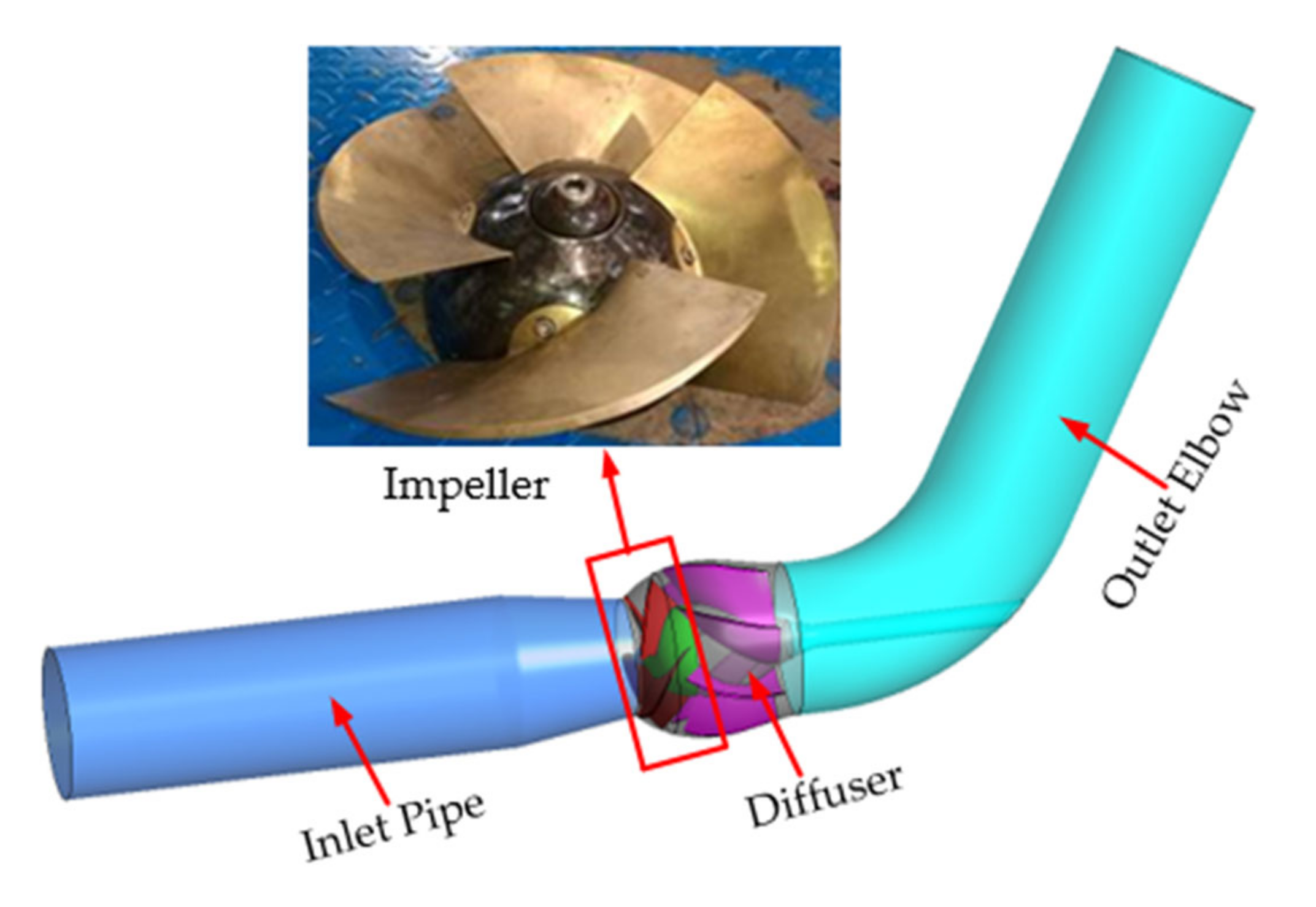
2. Model Description

A mixed flow pump with a specific speed of 511 was selected as the baseline model. The pump system is shown in Figure 1, consisting of a straight inlet pipe, an impeller, a vane diffuser, and an outlet elbow. The design specifications of the baseline model are shown in

Table 1. Design parameters of the baseline model.

Design flow rate (m3/s)	0.427	Design head (m)	12.66
Impeller diameter (mm)	320	Impeller blade number	4
Rotational speed (r/min)	1450	Specific speed	511
Minimum hub diameter (mm)	60	Maximum hub diameter (mm)	210
Minimum shroud diameter (mm)	270	Maximum shroud diameter (mm)	368

.

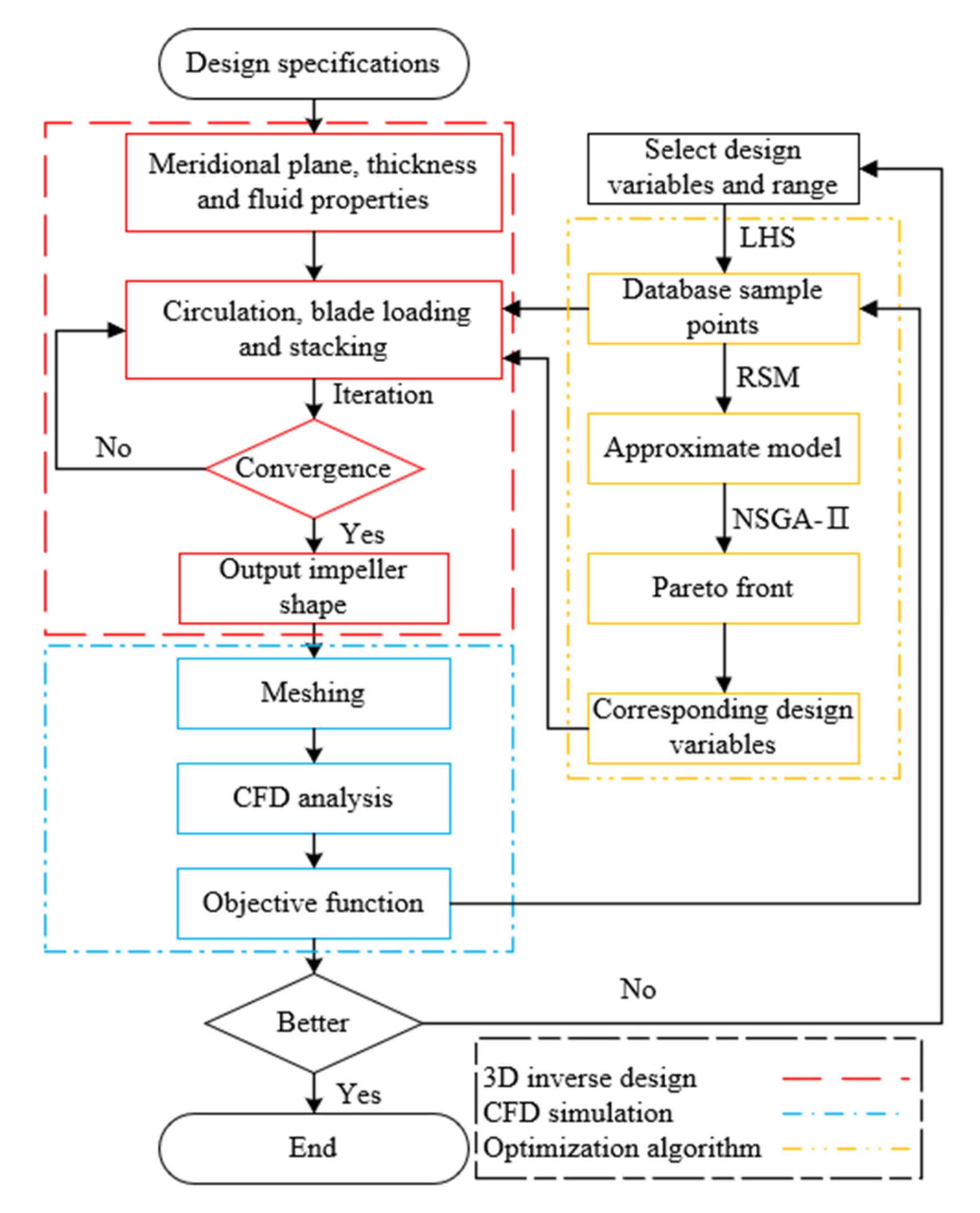
3. Optimization Design Strategy

A calculation flowchart of the comprehensive optimization system is shown in Figure 2. In this figure, IDM is used for blade parameterization and generation; CFD is used for impeller performance prediction; and non-dominated sorting genetic algorithm (NSGA-II), response surface model (RSM), and Latin hypercube sampling (LHS) are employed together to generate the multiple global optimal trade-off designs within an acceptable time scale.

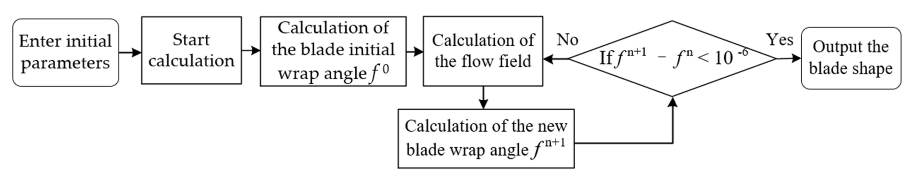
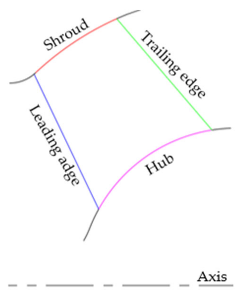
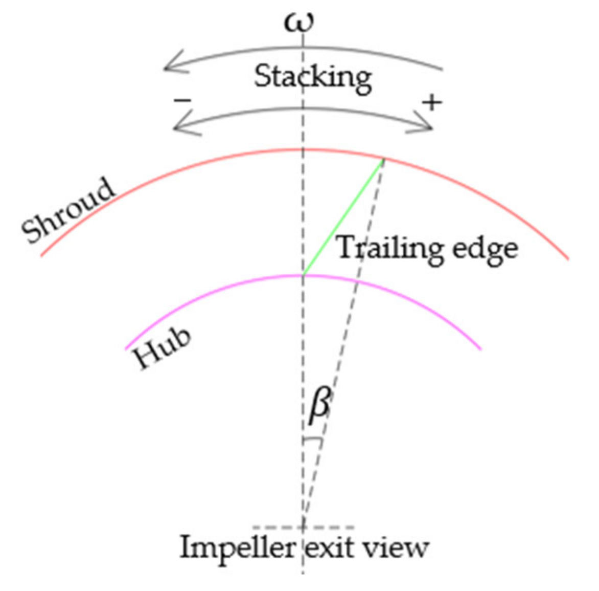
3.1. 3D Inverse Design Method

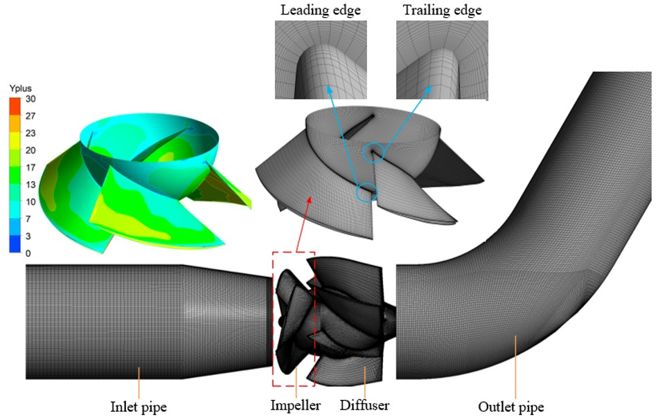
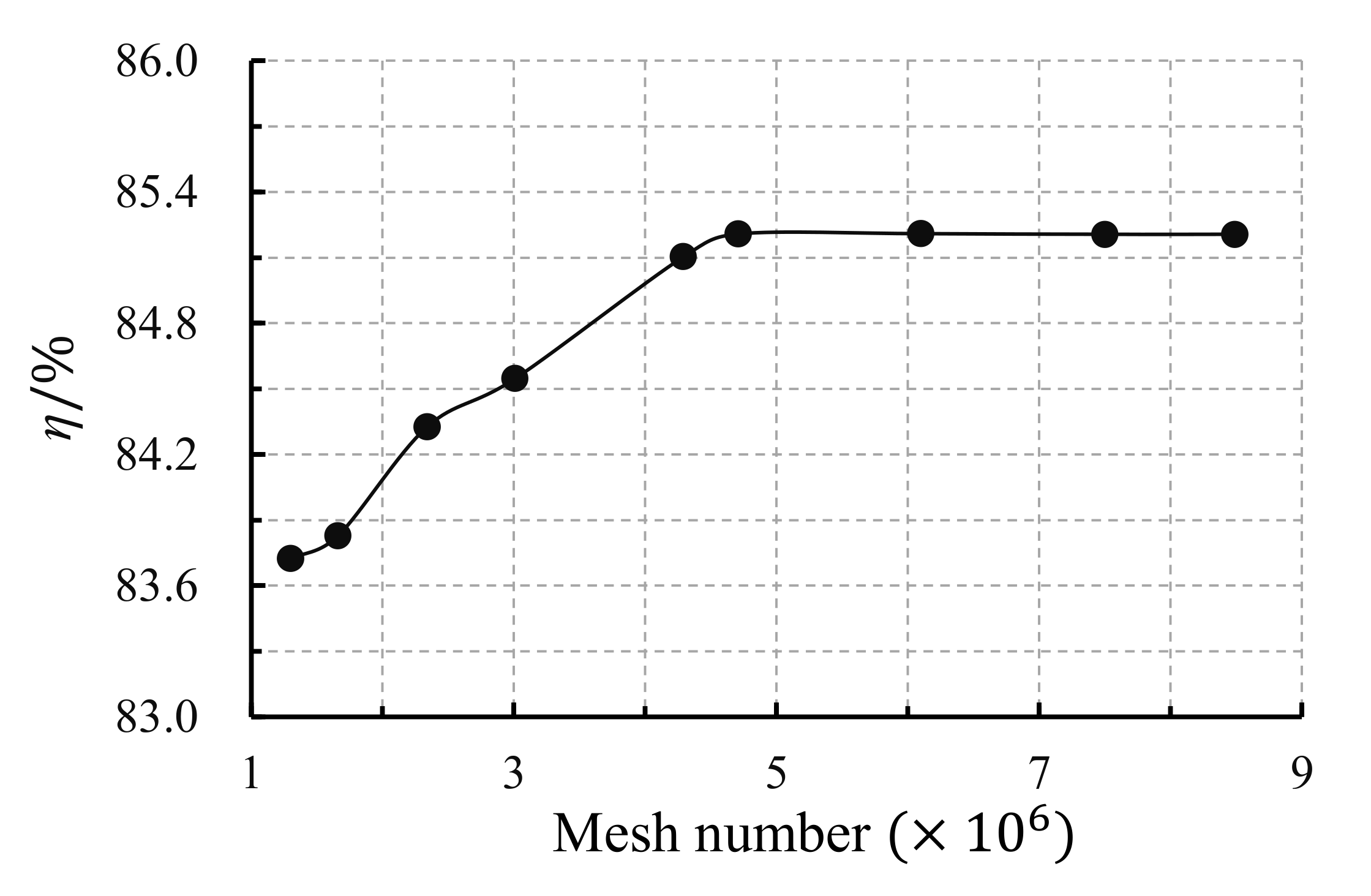
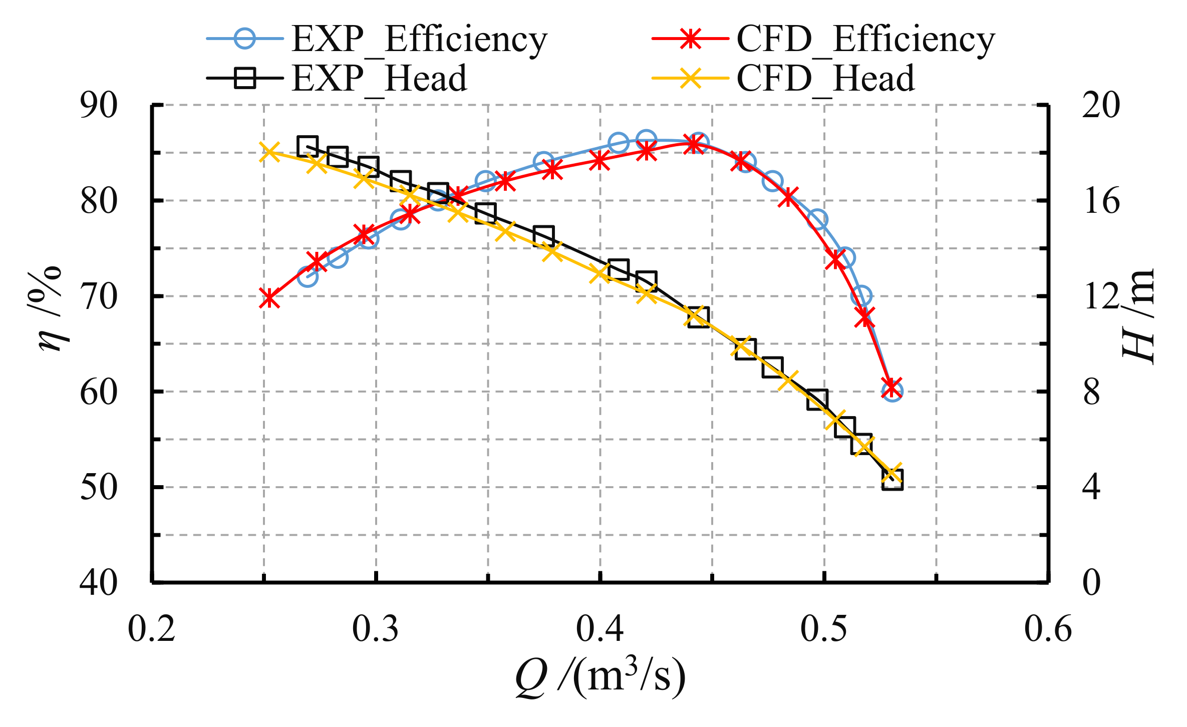
IDM was employed to parameterize the shape of the impeller. The flow through the impeller is assumed to be inviscid, incompressible, and steady. The blades are described by sheets of vorticity [27], and the strength is determined by the circulation $r\overline{V_{\theta }}$:

$$r\overline{V_{\theta }}=\frac{B}{2\mathsf{\pi }}{\displaystyle {\int }_0^{\frac{2\mathsf{\pi }}{B}}r{V}_{\theta }}\mathrm{d}\theta$$

(1)

where $B$ is the blade numbers, $\overline{V_{\theta }}$ is the circumferentially averaged tangential velocity, $V_{\theta }$ is the tangential velocity, and $r$ is the radial coordinate.

According to the incompressible potential flow theory [12], the pressure distribution is closely related to the meridional derivative of the circulation $\partial \left(r\overline{V_{\theta }}\right)/\partial m$:

$$\Delta p=p^{+}-p^{-}=\frac{2\mathsf{\pi }}{B}\rho W_{\mathrm{m}}\frac{\partial (r\overline{V_{\theta }})}{\partial m}$$

(2)

where $p^{-} \mathrm{and} p^{+}$ are the suction surface and working surface static pressure, respectively; $m$ is the normalized streamline distance; $W_m$ is the fluid relative velocity; $\rho$ is the density of the fluid; and $\partial \left(r\overline{V_{\theta }}\right)/\partial m$ is the blade loading. The blade shape can be calculated by Equation (3):

$$(\overline{V_z}+v_{zbl})\frac{\partial f}{\partial z}+(\overline{V_r}+v_{rbl})\frac{\partial f}{\partial r}=\frac{r\overline{V_{\theta }}}{r^2}+\frac{v_{\theta bl}}{r}-\omega$$

(3)

where $v$ and $\overline{V}$ are the periodic velocity and circumferential average velocity, respectively, and subscripts $z$ and $r$ represent the axial and radial components of velocity, respectively. $f$ is the blade wrap angle that is a $\theta$ value at the blade between the leading edge and trailing edge. To obtain the blade shape, the initial wrap angle $f^0$ needs to be known. In this method, the initial wrap angle was prescribed by the stacking condition. Figure 3 shows the IDM calculation flowchart.

3.2. CFD Analyses

In this study, calculation of the optimization objectives and verification of the optimized result were all completed by CFD. Thus, the credibility of the optimization results was determined by the accuracy of the CFD analyses. Therefore, 3D steady incompressible Reynolds-Averaged Navier–Stokes (RANS) equation was used in the simulation of the mixed flow pump. The governing equations are defined as follow:

$$\frac{\partial V_j}{\partial x_i}=0$$

(4)

$$\frac{\partial (V_i{V}_j)}{\partial x_j}=-\frac{1}{\rho }\frac{\partial p}{\partial x_i}+\vartheta \frac{{\partial }^2{V}_i}{\partial x_i{x}_j}+\frac{\partial {\tau }_{ij}}{\partial x_j}$$

(5)

where ${\tau }_{i,j}$ are the Reynolds stresses, $V$ is the time-average velocity, and $\vartheta$ is the kinematic viscosity. The RANS equation was solved by the Shear stress transport (SST) $k-\omega$ turbulence model because this model has the advantages of accurately calculating the internal flow pattern of the mixed flow pump impeller [28] and shows less sensitivity to Y+ [29]. A high-resolution scheme was used to solve the convection-diffusion equation. All the walls in the computational domains were considered as no-slip. The boundary conditions of the outlet and inlet were set as the “static pressure” and “mass flow rate”, respectively. “Frozen rotor” was adopted for data transfer between the rotating domain and the fixed domain, while “none” was adopted for data transfer between the fixed domains. The convergence criteria for all calculations was set as $5\times {10}^{-5}$.

The meshes quality and quantity have a great influence on the accuracy of CFD analyses [30]. Compared with unstructured mesh, structured mesh has the advantages of controllable quantity and quality. Therefore, the discretization of the entire computational domain was accomplished by structured meshes, as shown in Figure 4. ANSYS ICEM was employed in the mesh division of outlet and inlet pipes, and ANSYS TurboGrid was employed in the mesh division of vane diffuser and impeller. Figure 5 shows the result of the mesh independence check. The pump efficiency increased gradually with increasing number of meshes until $4.71\times {10}^6$, after which the pump efficiency remained basically unchanged. Therefore, the total number of meshes used in this study was $4.71\times {10}^6$. Meanwhile, the maximum Y+ on the impeller blade and hub was less than 30, as shown in Figure 4.

The experimental performance and numerical performance of the baseline model were compared to illustrate the reliability of the CFD analysis; the results are shown in Figure 6. The experimental performance of the baseline model was tested by the Tianjin experimental test bench, as shown in Figure 7. In this test bench, the flow rate was measured by the intelligent electromagnetic flowmeter with the measurement error at $<\pm 0.2\%$, the torque and rotation speed was measured by the intelligent torque speed sensor with the measurement error at $<\pm 0.1\%$, and the head was measured by the intelligent differential pressure transmitter with the measurement error at $<\pm 0.1\%$. The random uncertainty and overall uncertainty of the test bench were less than 0.1% and 0.3%, respectively. Figure 6 shows that the experimental results of pump head and efficiency are in good agreement with the numerical results in the whole flow range. The maximum deviations of the pump head and efficiency did not exceed 4% and 2%, respectively. Thus, the CFD simulation used in this study has sufficient accuracy to ensure reliability of the optimization results.

3.3. Latin Hypercube Sampling

LHS was employed in the DOE since it can generate orthogonally, random, and equiprobable distributed sample points in the design space [31]. Compared with the design space, the sample space constructed by LHS had the advantages of a controllable number of sample points and the structure was consistent with the design space, which was helpful to reduce the number of calculation times.

3.4. Response Surface Model

The functional relationships between design parameters and optimization objectives can be constructed by an approximate model. Compared with other approximate models, RSM uses polynomial to fit design parameters and optimization objectives, which has the advantages of sufficient mathematical theory, strong practicability, and wide application range [32]. In this study, second-order RSM was used to establish the functional relationship between the design parameters and optimization objectives:

$$y={\alpha }_0+{\displaystyle \sum _{i=1}^N{\alpha }_i{x}_i}+{\displaystyle \sum _{i=1}^N{\alpha }_{ii}{x}_i^2+}{\displaystyle \sum _{i\ne j}^N{\alpha }_{ij}{x}_i{x}_j}$$

(6)

where ${\alpha }_0$, ${\alpha }_i$, ${\alpha }_{ii}$, and ${\alpha }_{ij}$ are the undetermined coefficients and can be obtained by the least squares regression from the design parameters and optimization objectives and where $N$ represents the number of design parameters.

3.5. Non-Dominated Sorting Genetic Algorithm

NSGA-II was invoked for multi-objective optimization. This algorithm employs the concept of Pareto dominance to solve the multi-objective problem simultaneously [33]. The four important concepts in this optimization algorithm are “non-dominated sorting”, “crowding distance”, “mutation”, and “crossover”. “Non-dominated sorting” and “crowding distance” are used to improve the elitism of the strategy and to reduce the process complexity. “Crossover” and “mutation” are used to efficiently perform the search and to avoid local minima.

4. Optimization of the Mixed Flow Pump

4.1. Design Parameters

The meridional channel of the baseline impeller as shown in Figure 8 consists of the hub, shroud, leading edge, and trailing edge. In this study, no changes were made to the meridional channel. Therefore, the impeller can be parameterized by parameterization of the blade in the optimization process. As indicated in Section 3.1, blade loading, stacking, and circulation have the greatest influences on the shape and performance of the blades in IDM. Thus, they were selected to parameterize the blades.

The blade lean angle at the trailing edge of the blade was specified by the stacking condition. For mixed flow pump design, stacking usually was imposed linearly at the trailing edge, and proper stacking can effectively suppress the secondary flow [34]. As shown in Figure 9, when the blade lean corresponds to the rotation direction of the impeller, stacking $\beta$ is considered positive. In this case, the working capacity at the shroud will increase and the working capacity at the hub will decrease.

The Euler head of the impeller was determined by the difference in circulation distribution between the outlet and inlet of the impeller. In this study, the circulation at the impeller inlet was set to zero to satisfy the condition that the impeller inlet fluid has no pre-rotation and the circulation at the impeller outlet was described by the second-order parabolic:

$$r\overline{V_{\theta }}=b{r}^2+cr+d$$

(7)

where $b$, $c,$ and $d$ are the undetermined coefficients and can be calculated by the circulation values at the shroud, mid-span, and hub. In this study, the variables $r{V}_{\mathrm{h}}$ and $r{V}_{\mathrm{s}}$ (the value of $r\overline{V_{\theta }}$ at the hub and shroud, respectively) were selected as design parameters and $r{V}_{\mathrm{m}}$ (the value of $r\overline{V_{\theta }}$ at midspan) was automatically determined according to the impeller Euler’s head. Figure 10 shows two different forms of spanwise distributions of impeller exit circulation (SDIEC).

A typical combination curve, shown in Figure 11, was used to describe the distribution of blade loading along the hub and the shroud, and then, the linear interpolation method was used to calculate the blade loading distribution at other locations on the blade. For each streamline, the distribution of the blade loading was controlled by the following four parameters:$DRVT$, $NC$, $K$, and $ND$. $NC$ and $ND$ are the connection point locations; $K$ and $DRVT$ are the slope of linear line and the leading edge blade loading, respectively.

Therefore, the following eleven parameters are required for parameterization of the impeller:$\beta$, $r{V}_{\mathrm{h}}$, $r{V}_{\mathrm{s}}$, $DRV{T}_{\mathrm{s}}$, $K_{\mathrm{s}}$, $N{C}_{\mathrm{s}}$, $N{D}_{\mathrm{s}}$, $DRV{T}_{\mathrm{h}}$, $K_{\mathrm{h}}$, $N{C}_{\mathrm{h}}$, and $N{D}_{\mathrm{h}}$ (the subscripts $\mathrm{s}$ and $\mathrm{h}$ indicate shroud and hub, respectively).

4.2. Optimization Setting

The accuracy of RSM prediction is greatly affected by the number of design parameters $N$ and sampling points $S$. Generally, the minimum number of sampling points required for RSM is $S_{\min }=\frac{(N+s)!}{N!s!}$, where $s$ is the order of the interpolation. To improve the accuracy of RSM, the number of sampling points used in this study was $2S_{\min }$. As mentioned earlier, in the first optimization case, the influence of SDIEC was ignored, while in the second case, the influence of SDIEC was considered.

Table 2. Design parameters, constraints and optimization objectives for the two case.

	Parameters	First Case			Second Case
Type		Name	Variable	Range	Name	Variable	Range
Design Parameters		Blade Loading	$N{C}_{\mathrm{h}}$	0.1–0.5	Circulation	$R{V}_{\mathrm{h}}$	0.29–0.34
			$N{C}_{\mathrm{s}}$	0.1–0.5		$R{V}_{\mathrm{s}}$	0.29–0.34
			$DRV{T}_{\mathrm{h}}$	−0.25–0.25	Blade Loading	$DRV{T}_{\mathrm{h}}$	−0.25–0.25
			$N{D}_{\mathrm{h}}$	0.5–0.9		$N{D}_{\mathrm{h}}$	0.5–0.90
			$K_{\mathrm{h}}$	−2.0–2.0		$K_{\mathrm{h}}$	−2.0–2.0
			$DRV{T}_{\mathrm{s}}$	−0.25–0.25		$DRV{T}_{\mathrm{s}}$	−0.25–0.25
			$N{D}_{\mathrm{s}}$	0.5–0.9		$N{D}_{\mathrm{s}}$	0.5–0.90
			$K_{\mathrm{s}}$	−2.0–2.0		$K_{\mathrm{s}}$	−2.0–2.0
		Stacking	$\beta$	−20.0–20.0	Stacking	$\beta$	−20.0–20.0
Constraints		Pump efficiency at 1.0Qdes
		Pump head at 1.0Qdes
Objectives		Pump efficiency at $1.2Q_{\mathrm{des}}$
		Pump efficiency at $0.8Q_{\mathrm{des}}$

shows the design parameters, constraints, and optimization objectives for both cases.

In the first case, only the stacking condition and blade loading were adopted as design variables. To widen the mixed flow pump high-efficiency region, the pump efficiency at 1.2Q_des and 0.8Q_des were optimized. To ensure that the hydraulic performance of the optimized pump at the design point was truly better than that in the baseline model, the pump head and efficiency at the design point were set as constraints. The pump head and efficiency are calculated by Equations (8) and (9):

$$H= \frac{P_{\mathrm{out}}-P_{\mathrm{in}}}{\rho g}$$

(8)

$$\eta = \frac{\left(P_{\mathrm{out}}-P_{\mathrm{in}}\right)Q}{M\omega }$$

(9)

where $g$ represents the acceleration of gravity; $\rho$ represents the fluid density; $P_{\mathrm{in}}$ and $P_{\mathrm{out}}$ represent the inlet and outlet total pressures; $\omega$ represents the impeller angular velocity; and $M$ represents the torque acting on the impeller by the motor shaft.

In the second case, the influence of SDIEC on the optimization results was considered, and $r{V}_{\mathrm{h}}$ and $r{V}_{\mathrm{s}}$ were added to the design parameters as shown in Table 2. To reduce the number of calculation times, the two design parameters $N{C}_{\mathrm{h}}$ and $N{C}_{\mathrm{s}}$ were set as 0.18 and 0.10, respectively, because they have the least influence on the optimization objectives. Same as in the first case, the optimization targets were the pump efficiency at 1.2Q_des and 0.8Q_des and the constraints were the pump efficiency and head at the design point.

Therefore, to achieve the purpose of making the second-order RSM more accurate in both cases, 110 sample points were generated in each case. As shown in

Table 3. Parameters setting for non-dominated sorting genetic algorithm (NSGA-II).

Setting	Value
Number of generations	200
Population size	120
Cross distribution index	10
Crossover probability	0.9
Mutation distribution index	20
Initialization mode	Random

, parameter setting of NSGA-II was the same in both cases. A total of 24,000 impellers with different configurations were generated in each case.

4.3. Optimization Result

The Pareto front of the first case is shown in Figure 12. It is observed that, as the pump efficiency at 1.2Q_des decreases, the pump efficiency at 0.8Q_des increases, which means that there is a competitive relationship between the two optimization objectives. According to Equation (10), three different impeller configurations (F1–F3) were selected on the Pareto front for further study.

Figure 12. Pareto front of the first case.

Figure 12. Pareto front of the first case.

$$\mathrm{F}1: \left\{\begin{array}{c}\mathrm{M}\mathrm{a}\mathrm{x}\mathrm{i}\mathrm{m}\mathrm{i}\mathrm{z}\mathrm{e} {\eta }_{1.2}\\ {\eta }_{0.8}>80.48\end{array}\right.\hspace{1em}\mathrm{F}2: \left\{\begin{array}{c}\mathrm{M}\mathrm{a}\mathrm{x}\mathrm{i}\mathrm{m}\mathrm{i}\mathrm{z}\mathrm{e} \left( {\eta }_{1.2}+{\eta }_{0.8}\right)\\ {\eta }_{0.8}>80.48\\ {\eta }_{1.2}>73.84\end{array}\right.\hspace{1em}\mathrm{F}3: \left\{\begin{array}{c}\mathrm{M}\mathrm{a}\mathrm{x}\mathrm{i}\mathrm{m}\mathrm{i}\mathrm{z}\mathrm{e} {\eta }_{0.8}\\ {\eta }_{1.2}>73.84\end{array}\right.$$

(10)

The 3D shape comparison of impellers F1–F3 is shown in Figure 13a. In this figure, pink indicates impeller F1, blue indicates impeller F2, and red indicates impeller F3. It can be seen from Figure 13a that there are obvious differences in the shape of the blades of impellers F1–F3. The design parameters of optimized impellers F1–F3 are shown in

Table 4. Design parameters for the first case.

	Variables	$\mathit{D}\mathit{R}\mathit{V}{\mathit{T}}_{\mathit{h}}$	$\mathit{N}{\mathit{C}}_{\mathit{h}}$	${\mathit{K}}_{\mathit{h}}$	$\mathit{N}{\mathit{D}}_{\mathit{h}}$	$\mathit{D}\mathit{R}\mathit{V}{\mathit{T}}_{\mathit{s}}$	$\mathit{N}{\mathit{C}}_{\mathit{s}}$	${\mathit{K}}_{\mathit{s}}$	$\mathit{N}{\mathit{D}}_{\mathit{s}}$	$\mathit{\beta }$
Impeller
F1		0.034	0.179	−0.983	0.899	−0.131	0.111	1.491	0.500	−19.983
F2		−0.04	0.178	−0.674	0.542	0.165	0.100	1.558	0.500	−18.999
F3		−0.041	0.228	−0.508	0.764	−0.193	0.100	1.574	0.500	−17.996

, and the performance predicted by RSM and CFD are shown in

Table 5. Performance comparison for first case.

	Performance	RSM		CFD
Impeller		${\mathit{\eta }}_{0.8} (\%)$	${\mathit{\eta }}_{1.2} (\%)$	${\mathit{\eta }}_{0.8} (\%)$	${\mathit{\eta }}_{1.2} (\%)$	${\mathit{H}}_{1.0} \left(\mathbf{m}\right)$	${\mathit{\eta }}_{1.0} (\%)$
F1		80.52	79.96	80.54	80.32	12.31	87.62
F2		80.73	77.93	80.70	78.03	12.28	87.81
F3		80.80	76.45	80.77	76.25	12.34	87.99
Baseline model				80.48	73.84	12.10	85.21

. Here, the performance calculated by CFD agrees well with the RSM prediction. Compared with baseline impeller, the pump efficiency has been significantly improved under high flow conditions. However, under low flow conditions, the improvement is not very significant. Taking impeller F1 as an example, the pump efficiency at 1.2Q_des, 1.0Q_des, and 0.8Q_des are 80.32%, 87.62%, and 80.54%, respectively. These values correspond to 6.48%, 2.41%, and 0.06% improvement over the baseline impeller.

The Pareto front of the second case is shown in Figure 14. Same as in the first case, three different impeller configurations (S1–S3) were selected on the Pareto front. Figure 13b shows the 3D shape comparisons of impellers S1–S3. In this figure, pink indicates impeller S1, blue indicates impeller S2, and red indicates impeller S3.

Table 6. Design parameters for the second case.

	Parameters	$\mathit{R}{\mathit{V}}_{\mathit{h}}$	$\mathit{R}{\mathit{V}}_{\mathit{s}}$	$\mathit{D}\mathit{R}\mathit{V}{\mathit{T}}_{\mathit{h}}$	$\mathit{N}{\mathit{D}}_{\mathit{h}}$	${\mathit{K}}_{\mathit{h}}$	$\mathit{D}\mathit{R}\mathit{V}{\mathit{T}}_{\mathit{s}}$	$\mathit{N}{\mathit{D}}_{\mathit{s}}$	${\mathit{K}}_{\mathit{s}}$	$\mathit{\beta }$
Impeller
S1		0.3005	0.3365	0.249	0.513	−1.729	−0.144	0.706	1.999	−16.269
S2(Preferred)		0.3318	0.3363	0.199	0.893	−1.464	−0.088	0.503	−1.439	−13.804
S3		0.3129	0.3365	0.199	0.500	−1.50	−0.200	0.900	−1.499	−19.864

shows the design parameters of the optimized impellers S1–S3, and

Table 7. Performance comparison for the second case.

	Performance	RSM		CFD
Impeller		${\mathit{\eta }}_{0.8} (\%)$	${\mathit{\eta }}_{1.2} (\%)$	${\mathit{\eta }}_{0.8} (\%)$	${\mathit{\eta }}_{1.2} (\%)$	${\mathit{H}}_{1.0} \left(\mathbf{m}\right)$	${\mathit{\eta }}_{1.0} (\%)$
S1		80.68	83.10	80.87	82.54	12.52	88.4
S2 (Preferred)		81.23	80.75	81.75	81.08	12.18	88.87
S3		82.00	76.45	81.80	77.84	11.97	88.64
Baseline model				80.48	73.84	12.10	85.21

shows the performance predicted by RSM and CFD. Compared with the first case, all the optimization objectives were further improved in this case, especially at low flow conditions. Taking impeller S2 as an example, the pump efficiencies at 1.2Q_des, 1.0Q_des, and 0.8Q_des are 81.08%, 88.87%, and 81.75%, respectively. These efficiencies correspond to 7.24%, 3.66%, and 1.27% improvements over the baseline impeller.

5. Influence of SDIEC on Optimization Results

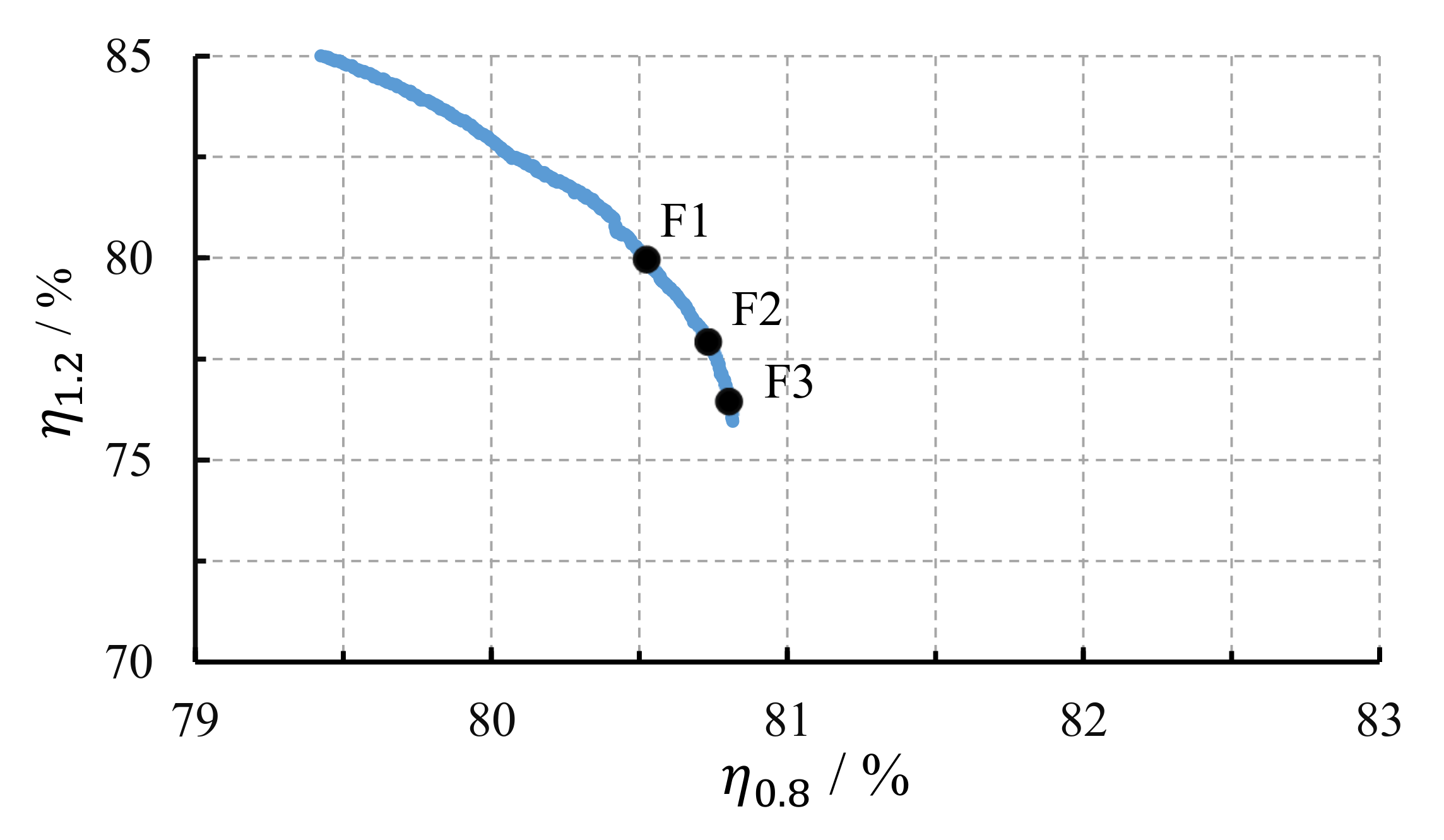
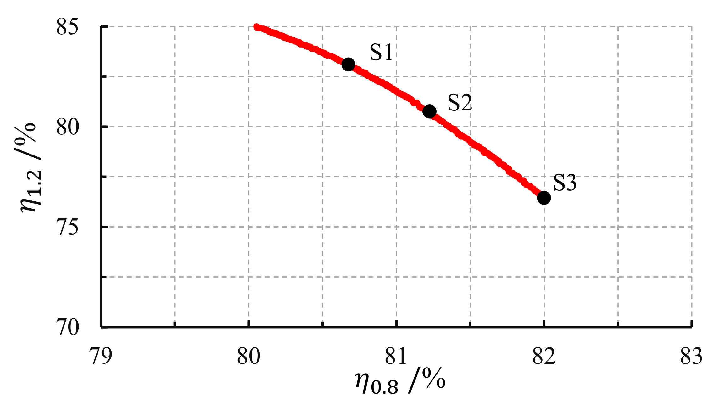
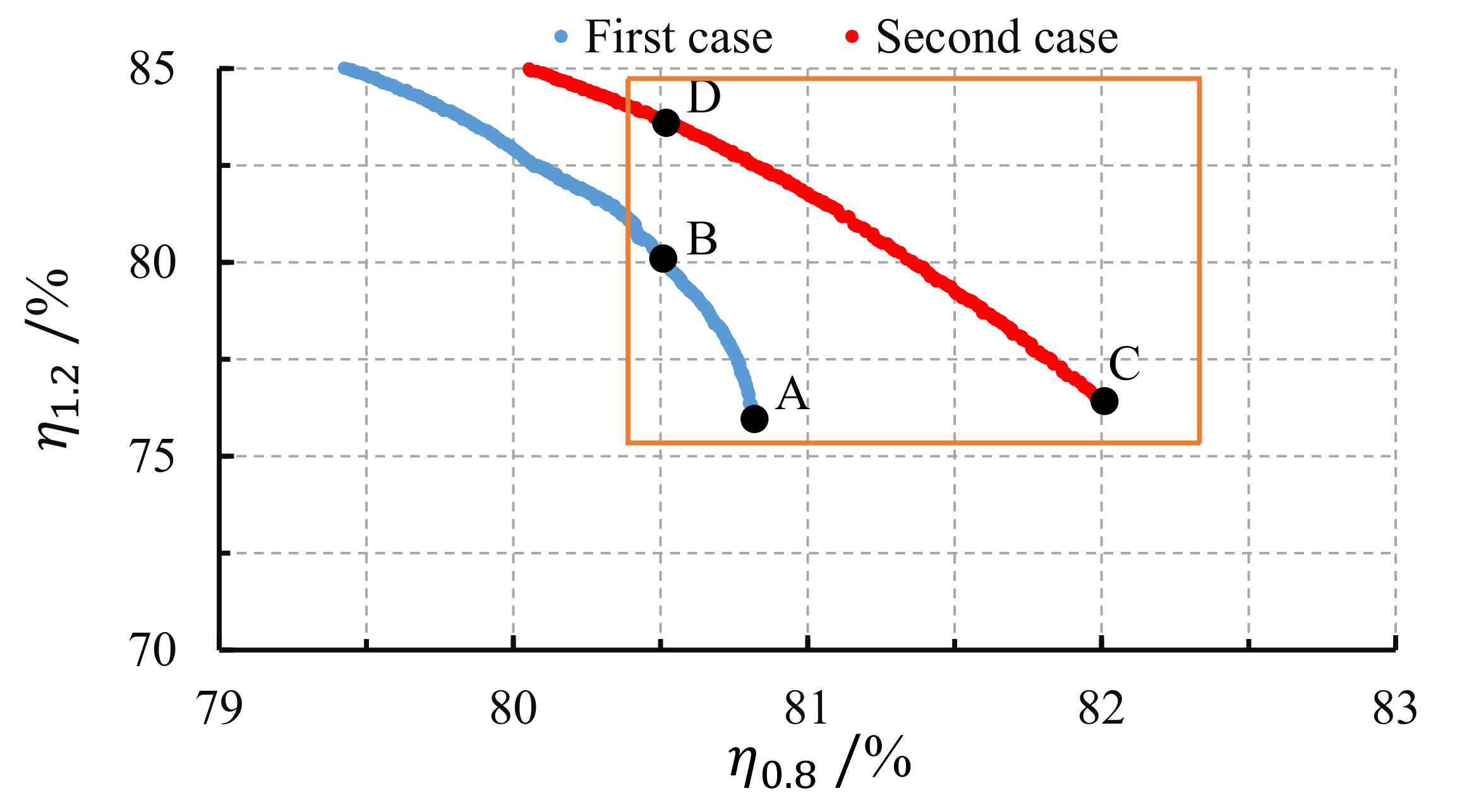
5.1. Comparison of Pareto Front for First and Second Case

The comparison of the Pareto front obtained from the first case and the second case is shown in Figure 15, where the impellers in the orange wireframe are the impellers that meet the optimization requirements. To illustrate the influence of SDIEC on the optimization results, impellers A, B, C, and D were selected for further study. By comparing impellers A and C, it can be seen that, when the influence of SDIEC was considered in the optimization process, the optimization upper limit under low flow conditions increased by 1.2%. By comparing impellers B and D, it can be seen that the optimization upper limit under high flow conditions increased by 3.5%. Besides, in the second case, with the increase of pump efficiency at low flow conditions, the reduction of pump efficiency at high flow conditions was smaller, which means that the impeller with good comprehensive performance was more likely to be obtained in the second case.

In summary, to further improve the mixed flow pump performance, it is necessary to consider the influence of SDIEC in the optimization process.

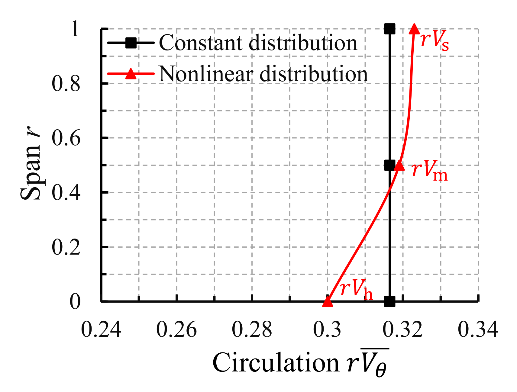
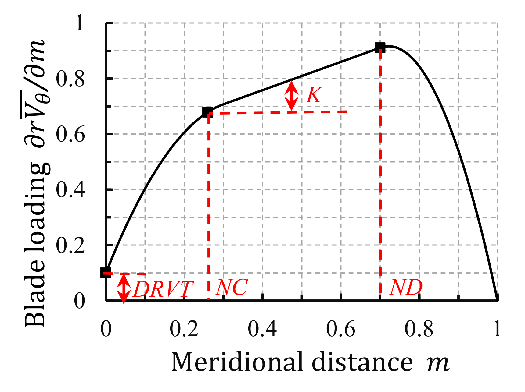
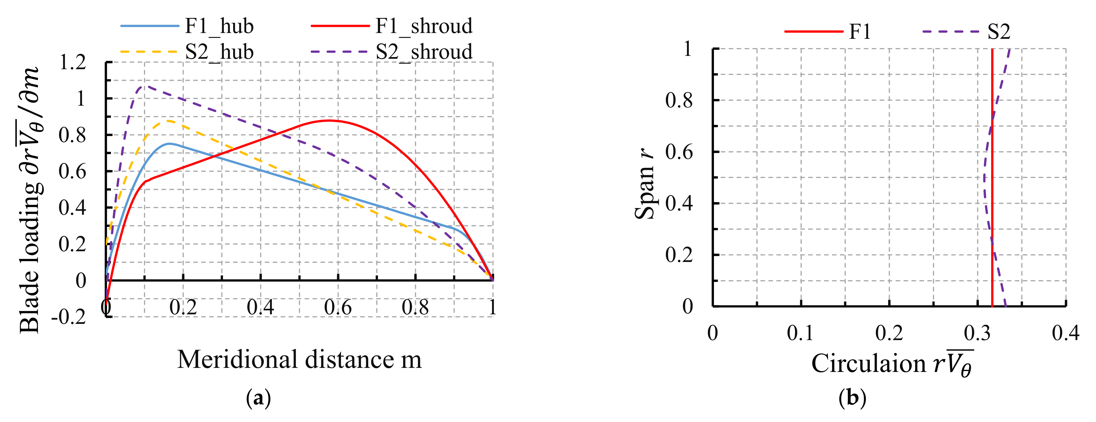
5.2. Comparison of Blade Loading and Circulation Distribution for the First and Second Cases

The optimized impellers F1 and S2 mentioned in Section 4.3 were selected as preferred impellers for the first and second cases, respectively. The blade loading distribution and SDIEC of impeller F1 and S2 are shown in Figure 16. In impeller F1, the SDIEC is uniform and the distributions of blade loading are aft-loaded and fore-loaded on the shroud and hub, respectively. However, in impeller S2, the SDIEC is a second-order parabolic and the blade loading at shroud and hub are both fore-loaded. Therefore, when SDIEC is considered in the optimization process, the blade loading and circulation distribution on the entire blade is greatly changed.

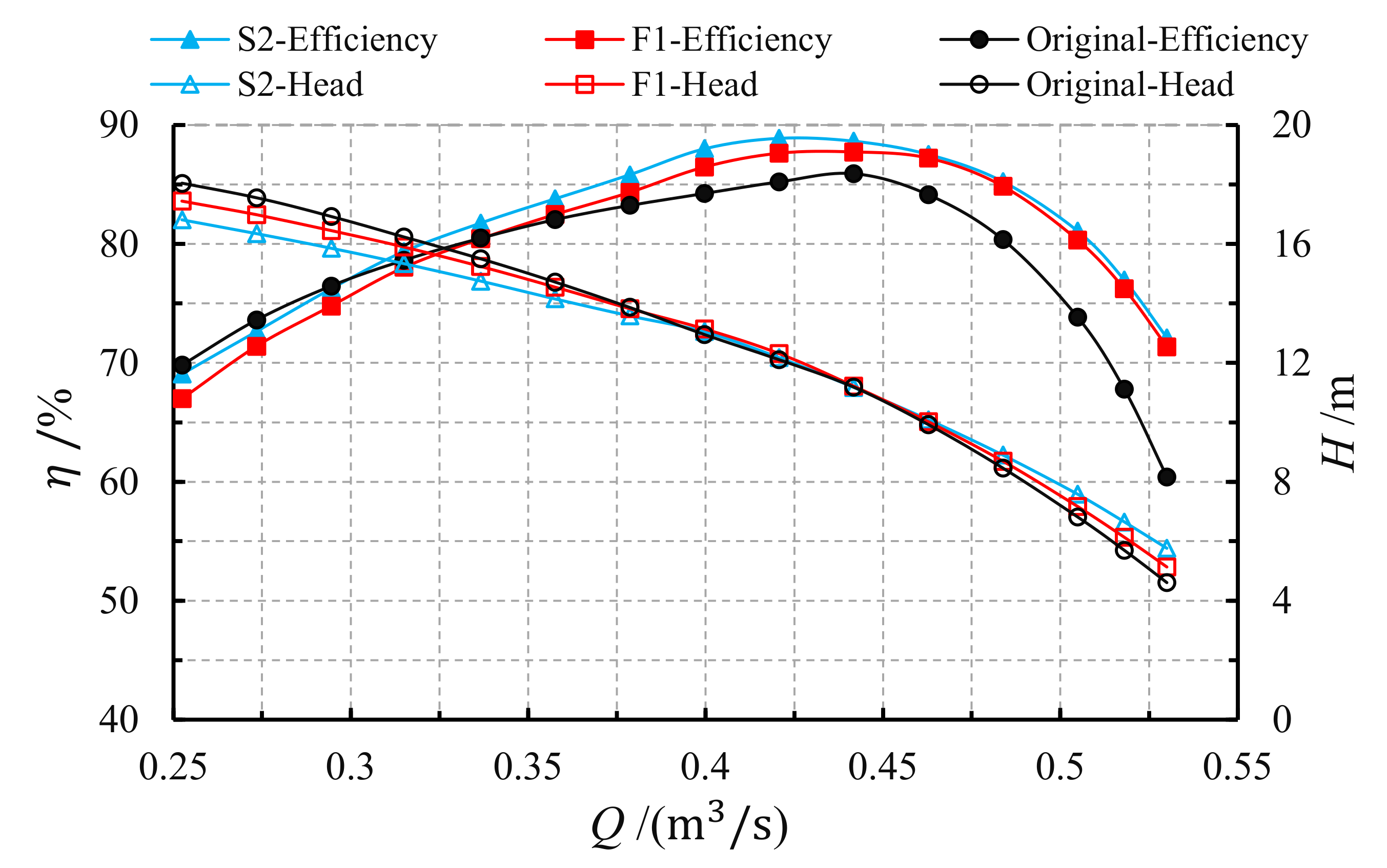
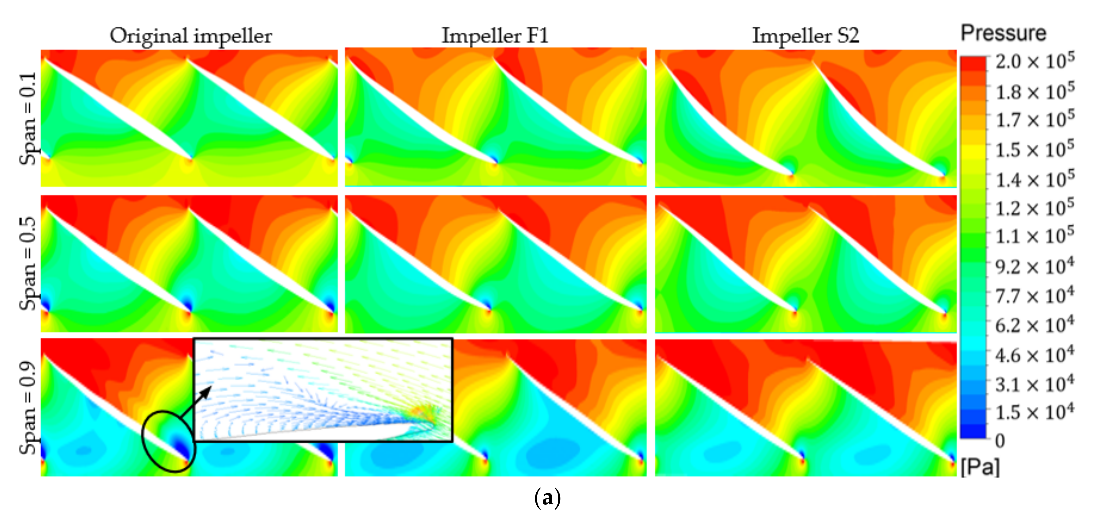
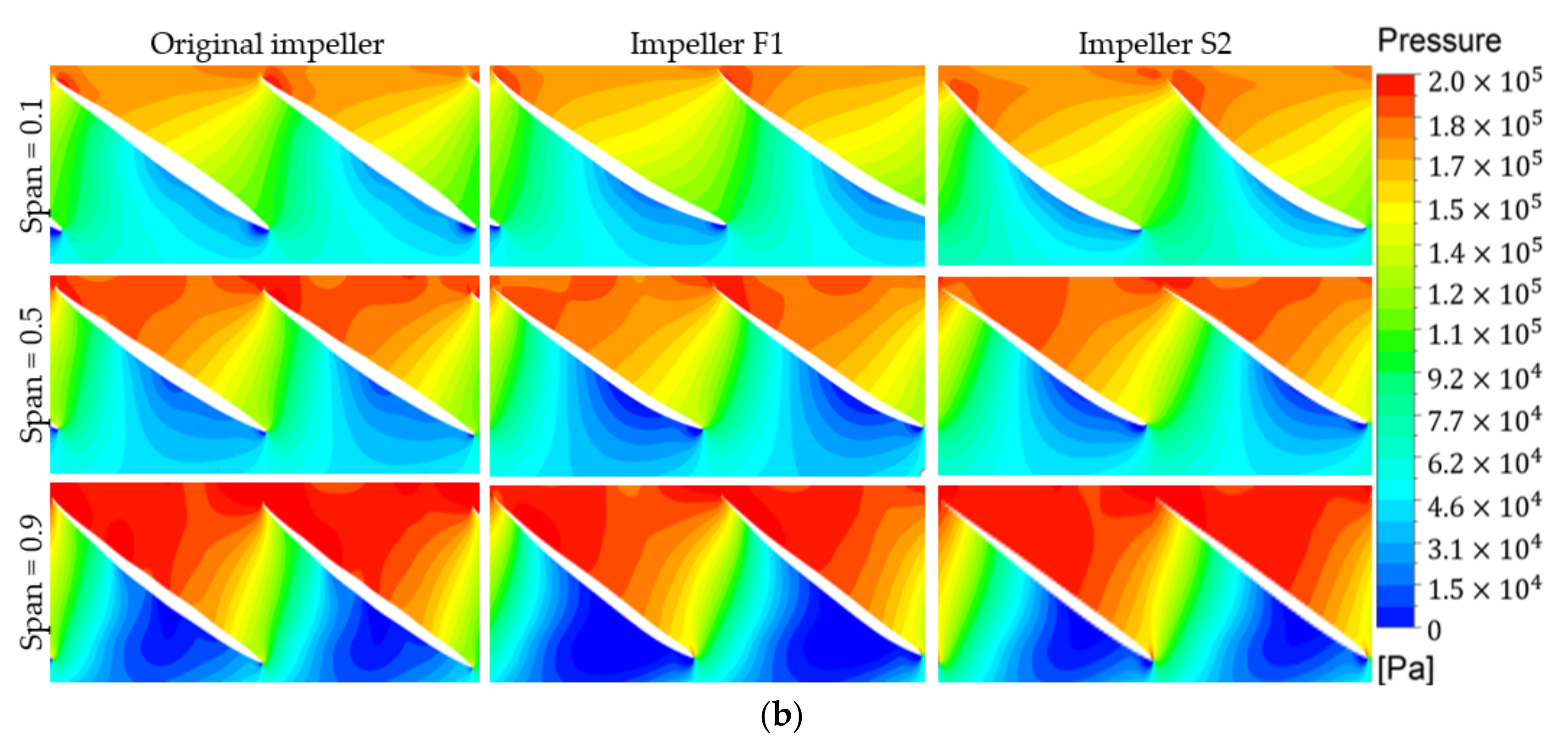
5.3. Performance Comparison Between Preferred Impellers and Baseline Impeller

The performance comparison between the preferred impellers F1 and S2 and the baseline impeller is shown in Figure 17. When the flow rate is greater than 0.8Q_des, the pump efficiency of the optimized impellers F1 and S2 is higher than that of the baseline model. However, compared with impeller F1, impeller S2 has a higher pump efficiency at all flow rates, especially at low flow conditions. The pump efficiencies of impeller S2 at 1.2Q_des, 1.0Q_des, and 0.8Q_des are increased by 0.76%, 1.24%, and 1.21%, respectively over impeller F1.

The pump head of the optimized impellers F1 and S2 presented an interesting change compared to the baseline impeller. The pump head of the optimized impellers F1 and S2 under the design condition are the same as the baseline impeller. However, under low flow conditions, the pump head of the baseline impeller is the highest, followed by the impeller F1, and the lower the flow rate, the greater the head difference. Under high flow conditions, the pump head shows an opposite trend to low flow conditions.

To clarify the optimization mechanism, it is necessary to compare and analyze the internal flow field of the model. The comparison of pressure contours between the baseline impeller and the preferred impellers F1 and S2 at 1.2Q_des and 0.8Q_des are shown in Figure 18. After carefully considering the influence of the wall on the flow field, these data were extracted at $r=0.9$, 0.5, and 0.1 respectively. As shown in Figure 18a, at 1.2Q_des, an obvious low-pressure region appeared on the leading edge near the shroud of the baseline impeller, which resulted in a large-scale backflow. After optimization, the low-pressure region was greatly weakened and the backflow was completely suppressed. Besides, the pressure distribution at the inlet of impeller S2 was more uniform than that of impeller F1. Figure 18b also shows the same phenomenon, but it should be noted that the low-pressure region appears on the blade suction surface and that there is no backflow in the low-pressure region.

6. Conclusions

In this study, the influence of SDIEC on the optimization results of mixed flow pump impeller was quantitatively studied by using the combined optimization system. During the optimization process, the impeller was parameterized by the inverse design method, the optimization objectives were the pump efficiencies at 1.2Q_des and 0.8Q_des, and the constraints were the pump head and efficiency at 1.0Q_des. The conclusions of this research are as follows:

(1)

In the first case, the influence of SDIEC was ignored in the optimization process and only the stacking condition and blade loading were used as design variables, but satisfactory results were still obtained. Taking optimized impeller F1 as an example, the pump efficiencies at 1.2Q_des, 1.0Q_des, and 0.8Q_des are 80.32%, 87.62%, and 80.54%, respectively. These values correspond to 6.48%, 2.41%, and 0.06% improvement over the baseline impeller.

(2)

In the second case, the influence of SDIEC was considered in the optimization process, and the stacking, blade loading, and circulation were used as the design variables and the upper limit of optimization was further improved. Taking optimized impeller S2 as an example, the pump efficiencies at 1.2Q_des, 1.0Q_des, and 0.8Q_des are 81.08%, 88.87%, and 81.75%, respectively. These values correspond to 0.76%, 1.24%, and 1.21% improvement over the impeller F1.

(3)

SDIEC also has a significant influence on the blade loading distribution of the optimized impeller. In impeller F1, the blade loading at the shroud and hub are aft-loaded and fore-loaded, respectively. While in impeller S2, the blade loading at the shroud and hub are both fore-loaded.

Based on the above findings, to further improve the optimization upper limit of the mixed flow pump, it is necessary to consider the influence of SDIEC in the optimization process. Additionally, the research results can provide guidance for the optimization of other rotating machinery.

References

1. Kim, J.H.; Kim, K.Y. Optimization of vane diffuser in a Mixed-flow pump for high efficiency design. In Proceedings of the 2010 International Conference on Pumps and Fans, Hangzhou, China, 18–21 October 2010. [Google Scholar]
2. Bing, H.; Cao, S.L.; Tan, L.; Zhu, B.S. Effects of meridional flow passage shape on hydraulic performance of mixed flow pump impellers. Chin. J. Mech. Eng. 2013, 3, 469–475. [Google Scholar] [CrossRef]
3. Si, Q.R.; Lu, R.; Shen, C.H.; Xia, S.J.; Sheng, G.C.; Yuan, J.P. An intelligent CFD-Based optimization system for fluid machinery: Automotive electronic pump case application. Appl. Sci. 2020, 10, 366. [Google Scholar] [CrossRef] [Green Version]
4. Ma, Z.; Zhu, B.S.; Rao, C.; Shangguan, Y.H. Comprehensive hydraulic improvement and parametric analysis of a Francis turbine runner. Energies 2019, 12, 307. [Google Scholar] [CrossRef] [Green Version]
5. Yong, Y.; Zhu, R.S.; Wang, D.Z.; Yin, J.L.; Li, T.B. Numerical and experimental investigation on the diffuser optimization of a reactor coolant pump with orthogonal test approach. J. Mech. Sci. Technol. 2016, 30, 4941–4948. [Google Scholar]
6. Liu, H.; Chen, X.; Wang, K.; Tan, M.; Zhou, X. Multi-condition optimization and experimental study of impeller blades in a mixed flow pump. Adv. Mech. Eng. 2016, 8. [Google Scholar] [CrossRef] [Green Version]
7. Meng, F.; Li, Y.; Yuan, S.; Wang, W.; Zheng, Y.; Osman, M.K. Multiobjective Combination Optimization of an Impeller and Diffuser in a Reversible Axial-Flow Pump Based on a Two-Layer Artificial Neural Network. Processes 2020, 8, 309. [Google Scholar] [CrossRef] [Green Version]
8. Zhu, Y.J.; Ju, Y.P.; Zhang, C.H. An Experience-independent Inverse Design Optimization Method of Compressor Cascade Airfoil. J. Power Energy 2018, 233, 431–442. [Google Scholar] [CrossRef]
9. Pei, J.; Gan, X.; Wang, W.; Yuan, S.; Tang, Y. Multi-objective shape optimization on the inlet pipe of a vertical inline pump. J. Fluids Eng. 2019, 141, 061108. [Google Scholar] [CrossRef]
10. Shim, H.S.; Afzal, A.; Kim, K.Y.; Jeong, H.S. Three-objective optimization of a centrifugal pump with double volute to minimize radial thrust at off-design conditions. Proc. Inst. Mech. Eng. Part A J. Power Energy. 2016, 230, 598–615. [Google Scholar] [CrossRef]
11. Yang, W.; Xiao, R.F. Multiobjective optimization design of a pump–turbine impeller based on an inverse design using a combination optimization strategy. J. Fluid. Eng. 2014, 136, 249–256. [Google Scholar] [CrossRef]
12. Zangeneh, M. A compressible three-dimensional design method for radial and mixed flow turbomachinery blades. Int. J. Numer. Methods Fluids 1991, 13, 599–624. [Google Scholar] [CrossRef]
13. Yin, J.; Wang, D. Review on applications of 3D inverse design method for pump. Chin. J. Mech. Eng. 2014, 27, 520–527. [Google Scholar] [CrossRef]
14. Zangeneh, M.; Goto, A.; Takemura, T. Suppression of Secondary Flows in a Mixed Flow Pump Impeller by Application of Three-Dimensional Inverse Design Method: Part 1—Design and Numerical Validation. J. Turbomach. 1996, 118, 536. [Google Scholar] [CrossRef]
15. Goto, A.; Takemura, T.; Zangeneh, M. Suppression of secondary flows in a mixed flow pump impeller by application of three-dimensional inverse design method: Part 2—Experimental validation. J. Turbomach. 1996, 118, 544–551. [Google Scholar] [CrossRef]
16. Huang, R.F.; Luo, X.W.; Ji, B.; Wang, P.; Yu, A.; Zhai, Z.H.; Zhou, J.J. Multi-objective optimization of a mixed flow pump impeller using modified NSGA-II algorithm. Sci. China Technol. Sci. 2015, 58, 2111–2130. [Google Scholar] [CrossRef]
17. Lu, Y.M.; Wang, X.F.; Wang, W.; Zhou, F.M. Application of the modified inverse design method in the optimization of the runner blade of a mixed flow pump. Chin. J. Mech. Eng. 2018, 31, 105. [Google Scholar] [CrossRef] [Green Version]
18. Zhu, B.; Wang, X.; Tan, L.; Zhou, D.; Zhao, Y.; Cao, S. Optimization design of a reversible pump–turbine runner with high efficiency and stability. Renew. Energy 2015, 81, 366–376. [Google Scholar] [CrossRef]
19. Zangeneh, M.; Mendonça, F.; Hahn, Y.; Cofer, J. 3D multi-disciplinary inverse design based optimization of a centrifugal compressor impeller. In Proceedings of the ASME. Turbo Expo: Power for Land Sea, and Air, Düsseldorf, Germany, 16–20 June 2014; Volume 2B. [Google Scholar]
20. Maillard, M.; Zangeneh, M. Application of 3D Inverse Design Based Multi-Objective Optimization of Axial Cooling Fan with Large Tip Gab; SAE Technical Paper; SAE International: Detroit, MI, USA, 2014. [Google Scholar]
21. Boselli, P.; Zangeneh, M. An Inverse Design Based Methodology for Rapid 3D Multi-objective/ multidisciplinary of Axial Turbines. In Proceedings of the ASME 2011 Turbo Expo: Turbine Technical Conference and Exposition, Vancouver, BC, Canada, 6–10 June 2011. [Google Scholar]
22. Chen, L. The Optimal Design Method of Axial Flow Pump Outlet Circumference Variation Law and Geometric Parameter Integration. Hydraul. Vane Pump. 1993, 1, 27. (In Chinese) [Google Scholar]
23. Lang, J. Preliminary study of the optimal distribution law of axial-flow pump impeller axial speed and circulation. Fluid Mach. 1990, 31. (In Chinese) [Google Scholar]
24. Zhang, D.; Li, T.; Shi, W.; Zhang, H.; Zhang, G. Experimental investigation of meridional velocity and circulation in axial-flow impeller outlet. Trans. Chin. Soc. Agric. Eng. 2012, 28, 73–77. (In Chinese) [Google Scholar]
25. Zhang, D.; Shi, W.; Li, T.; Gao, X.; Guan, X. Establishment and Experiment on Nonlinear Circulation Mathematical Model of Axial Flow Pump Impeller. Trans. Chin. Soc. Agric. Mach. 2013, 44, 58–61. (In Chinese) [Google Scholar]
26. Wang, M.C.; Li, Y.J.; Yuan, J.P.; Meng, F.; Appiah, D.; Chen, J.Q. Comprehensive improvement of mixed flow pump impeller based on multi-objective optimization. Processes 2020, 8, 905. [Google Scholar] [CrossRef]
27. Hawthorne, W.R.; Wang, C.; Tan, C.S.; Mccune, J.E. Theory of blade design for large deflections: Part Ⅰ—Two-dimensional cascade. J. Eng. Gas. Turb. Power. 1984, 106, 346–353. [Google Scholar] [CrossRef]
28. Hellsten, A.; Laine, S. Extension of the k-omega-SST turbulence model for flows over rough surfaces. In Proceedings of the 22nd Atmospheric Flight Mechanics Conference, New Orleans, LA, USA, 11–13 August 1997. [Google Scholar]
29. Menter, F.; Ferreira, J.C.; Esch, T.; Konno, B.; Germany, A.C. The SST Turbulence Model with Improved Wall Treatment for Heat Transfer Predictions in Gas Turbines. In Proceedings of the International Gas Turbine Congress 2003, Tokyo, Japan, 2–7 November 2003. [Google Scholar]
30. Shim, H.S.; Kim, K.Y.; Choi, Y.S. Three-objective optimization of a centrifugal pump to reduce flow recirculation and cavitation. J. Fluids Eng. 2018, 140, 091202. [Google Scholar] [CrossRef]
31. Pebesma, E.J.; Gerard, B.M.H. Latin hypercube sampling of Gaussian random fields. Technometrics 1999, 41, 303–312. [Google Scholar] [CrossRef]
32. Khuri, A.I.; Mukhopadhyay, S. Response surface methodology. Wiley Interdiscip. Rev. Comput. Stat. 2010, 2, 128–149. [Google Scholar] [CrossRef]
33. Deb, K.; Agrawal, S.; Pratap, A.; Meyarivan, T. A fast elitist non-dominated sorting genetic algorithm for multi-objective optimization: NSGA-II. Lect. Notes Comput. Sci. 1917, 2000, 849–858. [Google Scholar]
34. Zhu, B.; Tan, L.; Wang, X.; Ma, Z. Investigation on flow characteristics of pump-turbine runners with large blade lean. J. Fluids Eng. 2017, 140, 031101. [Google Scholar] [CrossRef]
Figure 1. Baseline impeller.
Applsci 11 00507 g001
Figure 2. Optimization system.
Applsci 11 00507 g002
Figure 3. Three-dimensional inverse design method flowchart.
Applsci 11 00507 g003
Figure 4. Mesh of the computational domains.
Applsci 11 00507 g004
Figure 5. Mesh independence check.
Applsci 11 00507 g005
Figure 6. Comparison of simulation and experimental performance.
Applsci 11 00507 g006
Figure 7. The Tianjin experimental test bench.
Applsci 11 00507 g007
Figure 8. Meridional channel.
Applsci 11 00507 g008
Figure 9. Stacking condition.
Applsci 11 00507 g009
Figure 10. Impeller exit circulation distribution.
Applsci 11 00507 g010
Figure 11. Blade loading distribution.
Applsci 11 00507 g011
Figure 13. Geometry of the optimized impeller: (a) first case; (b) second case.
Applsci 11 00507 g013
Figure 14. Pareto front of the second case.
Applsci 11 00507 g014
Figure 15. Comparison of Pareto front for the first and second cases.
Applsci 11 00507 g015
Figure 16. Comparison of the circulation distribution of impellers F1 and S2: (a) blade loading distribution; (b) spanwise distribution of impeller exit circulation (SDIEC) distribution
Applsci 11 00507 g016
Figure 17. Comparison of external characteristics.
Applsci 11 00507 g017
Figure 18. Pressure distribution at different spans: (a) 1.2 Q des ; (b) 0.8 Q des .
Applsci 11 00507 g018aApplsci 11 00507 g018b