Application of PCSWMM for the 1-D and 1-D–2-D Modeling of Urban Flooding in Damansara Catchment, Malaysia

Abstract

Coupled with climate change, the urbanization-driven increase in the frequency and intensity of floods can be seen in both developing and developed countries, and Malaysia is no exemption. As part of flood hazard mitigation, this study aimed to simulate the urban flood scenarios in Malaysia’s urbanized catchments. The flood simulation was performed using the Personal Computer Storm Water Management Model (PCSWMM) modeling of the Damansara catchment as a case study. An integrated hydrologic-hydraulic model was developed for the 1-D river flow modeling and 1-D–2-D drainage overflow modeling. The reliability of the 1-D river flow model was confirmed through the calibration and validation, in which the water level in TTDI Jaya was satisfactorily predicted, supported by the coefficient of determination (R²), Nash–Sutcliffe model efficiency coefficient (NSE), and relative error (RE). The performance of the 1-D–2-D model was further demonstrated based on the flood depth, extent, and risk caused by the drainage overflow. Two scenarios were tested, and the comparison results showed that the current drainage effectively reduced the drainage overflow due to the increased size of drains compared to the historic drainage in 2015. The procedure and findings of this study could serve as references for the application in flood mitigation planning worldwide, especially for developing countries.

1. Introduction

Flood, coupled with climate change and urban development, is by far the most common natural disaster. Over the past few decades, a trend towards increasing frequency in flood events has been observed globally in response to rapid urbanization [1,2]. The conversion of a natural catchment to an urbanized catchment usually increases the impermeable surfaces, reducing ground infiltration and increasing the surface runoff rates [3]. This phenomenon leads to urban flood issues arising from insufficient flow capacities of rivers or drainage, especially during extreme precipitation events. An urban flood can be catastrophic, depending on the level of urbanization within a catchment. Therefore, it is necessary to manage urban growth sustainably to reduce the impact of urban flooding.

Malaysia is one of the rapidly developing countries in Southeast Asia and its urbanization has increased by almost 30% to 40% over the last few decades [4]. Being located near the equatorial doldrums, Malaysia experiences heavy rainfall throughout the year, with an annual average rainfall of 2500 mm for Peninsular Malaysia and 3250 mm for East Malaysia (Sabah and Sarawak) [5]. Consequently, Malaysia has frequently suffered from flooding during the monsoon period [6]. In the early 21st century, urbanization in Malaysia’s urban areas, notably the Damansara catchment, is expanding to accommodate nearly 226,000 residents [7]. According to the flood report of DID [8], severe flood events were reported within the Damansara catchment in 2015, the summary statistics of which are shown in

Table 1. Descriptive statistics of 2015 flood events in Damansara catchment.

	Average Total Precipitation (mm)	Flood Duration (h)	Lowest Flood Depth (m)	Highest Flood Depth (m)	Flood Extent (km2)
Mean	70.85	1.92	0.26	0.62	0.37
Median	71.00	2.00	0.30	0.55	0.03
Standard deviation	24.86	0.77	0.18	0.30	1.20
Minimum	31.00	0.50	0.10	0.30	0.00
Maximum	104.00	3.50	0.60	1.00	5.00
Sum	2338.00	36.50	8.20	19.80	12.27
Count	33	19	32	32	33

. Commonly, two types of flooding, namely fluvial floods (river floods) and pluvial floods (surface water floods), possibly occur following intense or prolonged rainfall. The former fluvial flood occurs when a river exceeds its capacity and overflows its bank. In contrast, the pluvial flood is distinguished by a surface water flood caused by insufficient drainage capacity. The Malaysian government has raised concerns over the urban flooding issues and much attention has been given to the flood mitigation and drainage system upgrading works, particularly around Kampung Melayu Subang [9].

Flood forecasting is the key non-structural measure for flood mitigation that has been recently implemented worldwide, typically involving an integrated hydrologic-hydraulic modeling approach. The Storm Water Management Model (SWMM) is a widely used urban stormwater model developed by the United States Environmental Protection Agency (US EPA) [10]. SWMM has a wide range of applications, including hydrologic impact assessment [11,12,13,14,15], catchment discretization [16], runoff quantity and quality modeling for short- or long-term periods [17,18,19], and urban floods and drainage modeling [20,21,22,23,24]. However, the lack of spatial interface poses tremendous challenges to SWMM models due to the complexity of urban areas. Hence, a commercial version of SWMM known as Personal Computer Storm Water Management Model (PCSWMM) is used, incorporating a stand-alone Geographic Information System (GIS) for integrated 1-D–2-D and quasi-2-D modeling. The reliability and efficiency of PCSWMM have garnered popularity in many countries, such as Korea [25], Cambodia [26,27], Norway [28], China [29], Thailand [30], the United States [31], Australia [32], the Philippines [33], and India [34]. In Malaysia, SWMM modeling with PCSWMM is less commonly done, though Hasan et al. [35] and Sidek et al. [36] used a different version of the stormwater modelling tool, XPSWMM, developed by XP Solutions to investigate the hydrological and hydraulic characteristics of the Aur River and Jeluh River catchments, respectively. This study, thus, aimed to provide the basis for flood modeling and risk mapping using PCSWMM.

In this framework, PCSWMM was applied for the simulation of 2015 historical urban flood events in the Damansara catchment. The model’s performance was evaluated through the 1-D river flow modeling and 1-D–2-D drainage overflow modeling. Additionally, the current drainage of the study area was investigated to determine if the size of current drains can delimit the flooded areas. In the last part of this study, flood risk maps were generated for historical and current drainage scenarios with different capacities. The presented methodologies could serve as a guide to PCSWMM modeling in (1) developing a 1-D model, (2) coupling 1-D and 2-D models, and (3) mapping the risk in food-prone areas. This paper is organized as follows: methodologies in terms of the study area, data collection, and model setup are first presented in Section 2. Section 3 presents the 1-D modeling for river flow and comparison with the historical data. This is followed by the 1-D–2-D drainage overflow modeling and risk mapping in Section 4. In Section 5, conclusions are drawn from the study, with some considerations for future work.

2. Materials and Methods

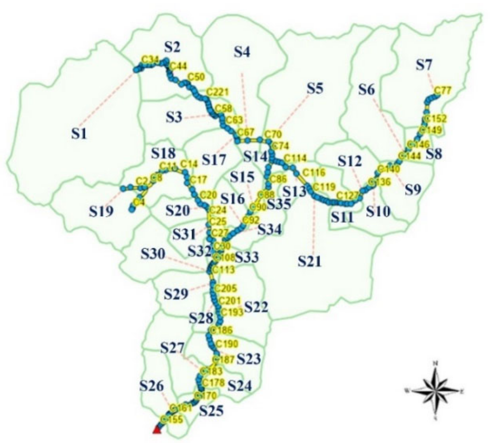
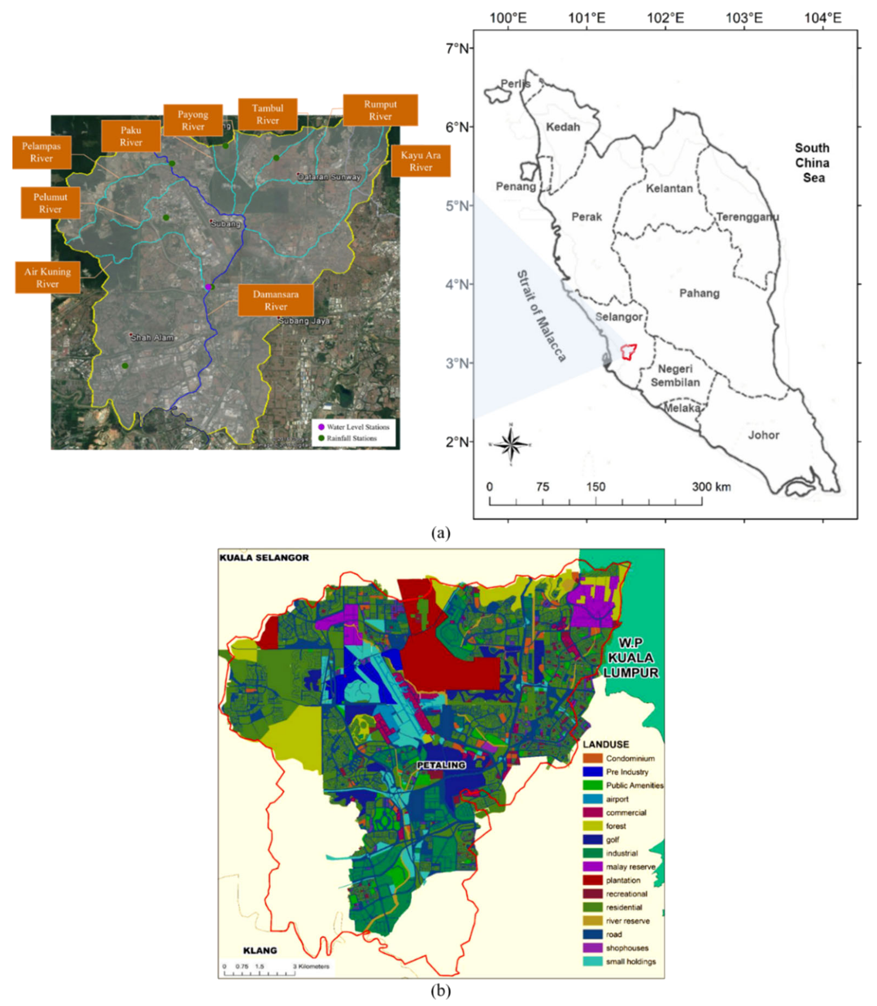
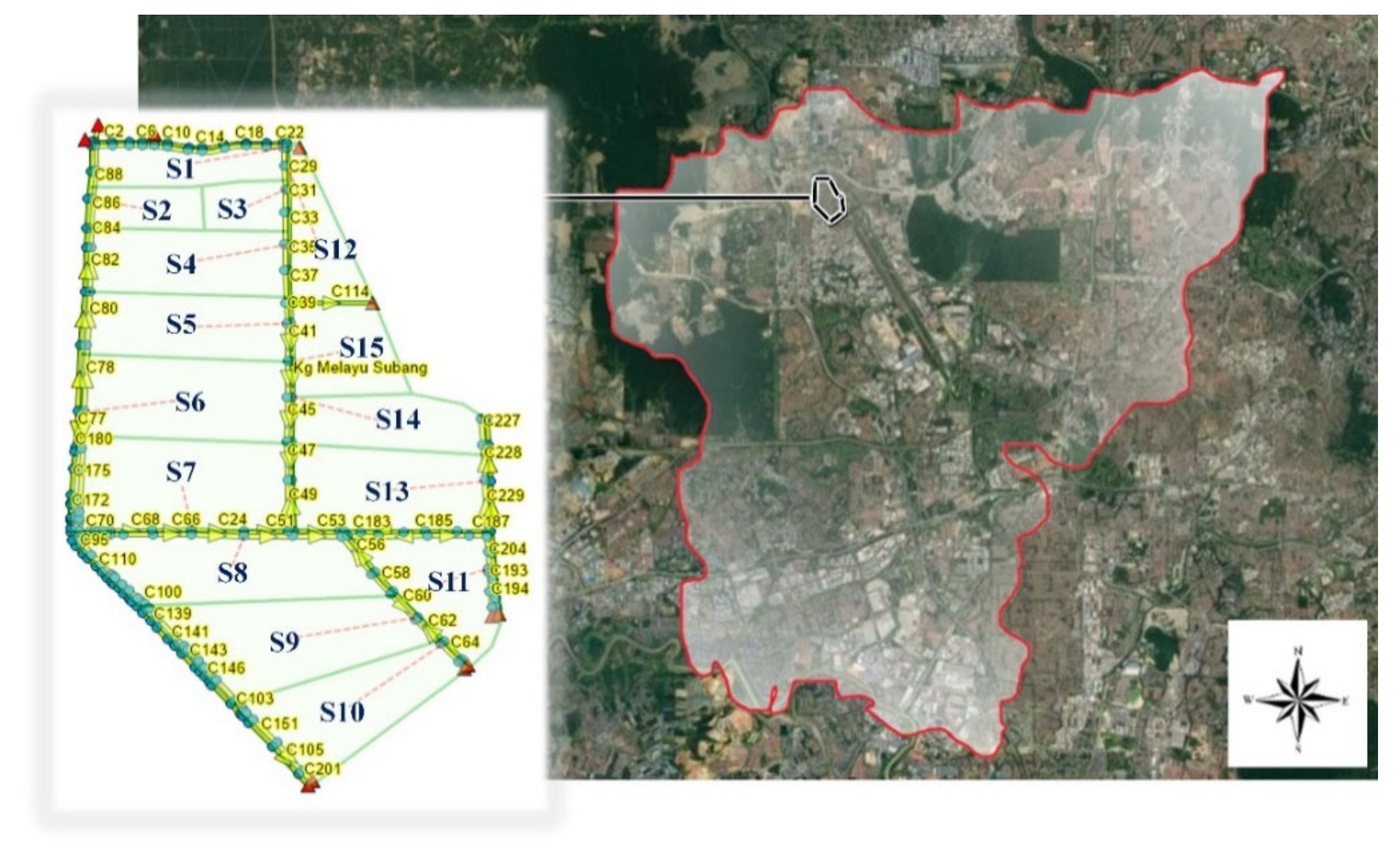
2.1. Site Description

The Damansara catchment is in the state of Selangor, located at the west coast of Peninsular Malaysia, as shown in Figure 1a. The main channel originates from the northern side of Sungai Buloh to Shah Alam and is known as the Damansara River. The Damansara River has six major tributaries, which are Pelumut River, Pelampas River, Payong River, Rumput River, Kayu Ara River, and Air Kuning River. The whole catchment is a part of the Klang river basin, with a total area of approximately 157 km², discharging into the Klang River at a river length of 20.8 km. The distribution of land use in the Damansara catchment is graphically presented in Figure 1b. The catchment has reached an urbanization level of approximately 76.9%, mainly dominated by residential, industrial, and commercial uses, such as the Shah Alam Stadium and Bukit Jelutong Business and Technology Centre. The intensive urban growth in the Damansara catchment has increased the risks of flood damage, especially at the river’s upstream areas near Kampung Melayu Subang and in the southern floodplains, comprising Taman Sri Muda, TTDI Jaya, and Batu 3 Shah Alam [8].

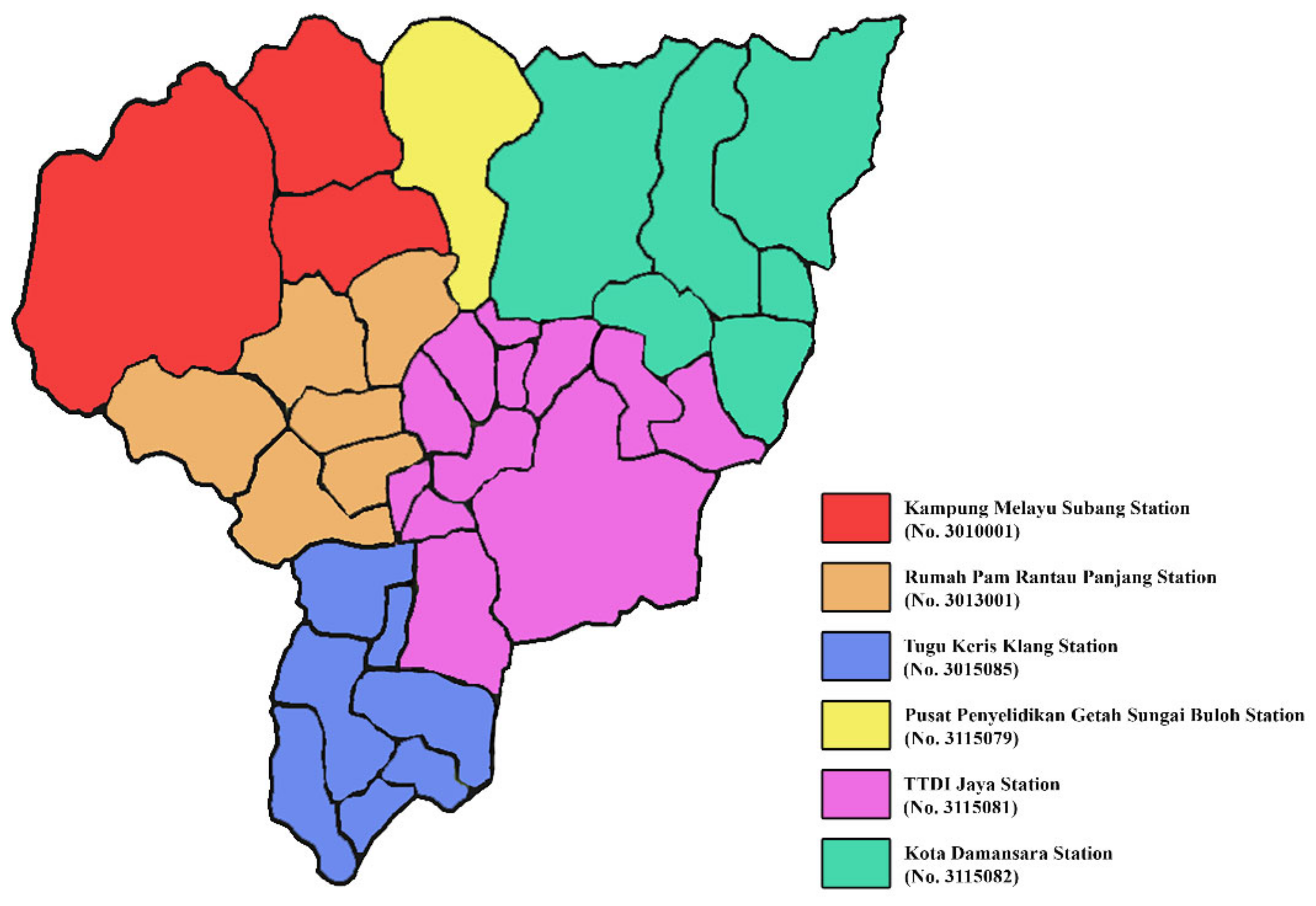
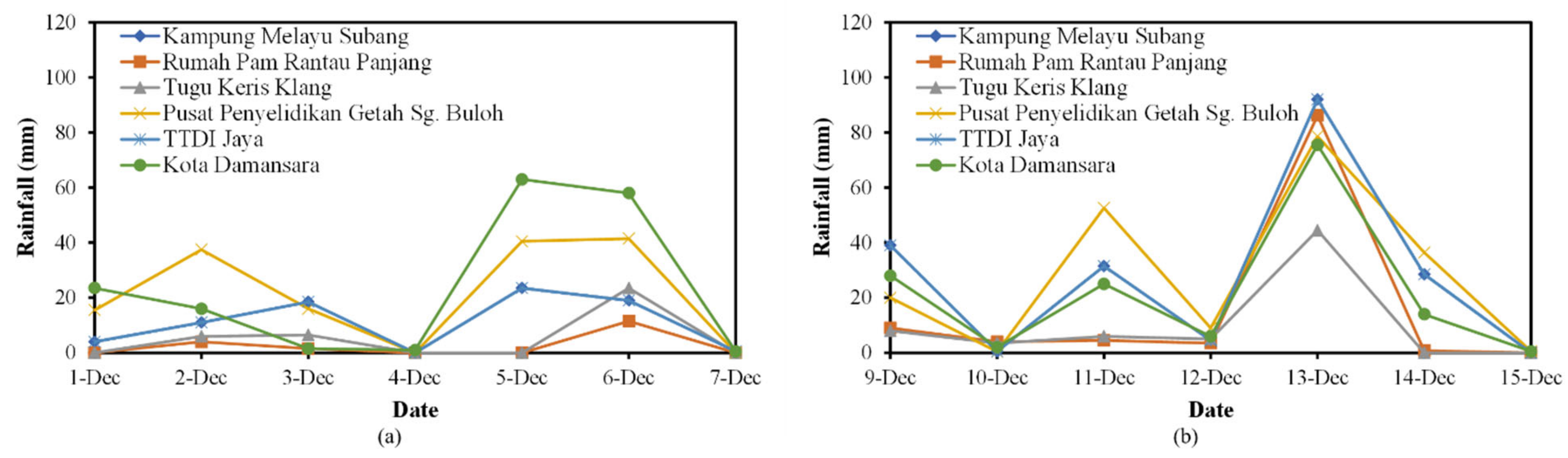
2.2. Precipitation and Streamflow Data Collection

The availability of meteorological stations, including the precipitation and streamflow gauging stations around the Damansara catchment, is shown in

Table 2. Summary statistics of daily recorded rainfall series in Damansara catchment (2009–2019).

Rainfall Station No.	Water Level Station No.	Station Name	Latitude	Longitude	Standard Deviation	Skewness	Kurtosis	Maximum Rainfall
3010001	-	Kampung Melayu Subang	03°09′29″	101°32′04″	14.05	3.23	13.41	134.50
3013001	-	Rumah Pam Rantau Panjang	03°07′51″	101°31′59″	13.40	3.63	18.71	171.40
3015085	-	Tugu Keris Klang	03°03′29″	101°30′59″	12.44	3.79	18.36	116.60
3115079	-	Pusat Penyelidikan Getah Sungai Buloh	03°10′02″	101°33′35″	14.67	2.84	9.57	113.50
3115081	3015490	TTDI Jaya	03°06′18″	101°33′49″	15.42	3.20	12.79	143.50
3115082	-	Kota Damansara	03°09′39″	101°34′59″	15.22	2.92	10.04	123.40

Note: Standard deviation and maximum rainfall are in mm.

. Ten-year meteorological data at stations (from the year 2009 to 2019) were obtained from the Department of Irrigation and Drainage (DID), Malaysia. The Damansara catchment experiences copious rain throughout the year, with an average annual rainfall depth of more than 2200 mm. The highest daily recorded depth varies from 113.5 to 171.4 mm for the six rainfall stations within the Damansara catchment (Table 2). The consistency of rainfall data was verified using a double mass curve [37]. In the double mass curve analysis, the cumulative annual rainfall at each station was plotted against the accumulations of the average values of annual rainfall recorded by the nearby stations. For all six rainfall stations in the catchment, the consistency of the recorded rainfall data was confirmed, with R² values close to 1.

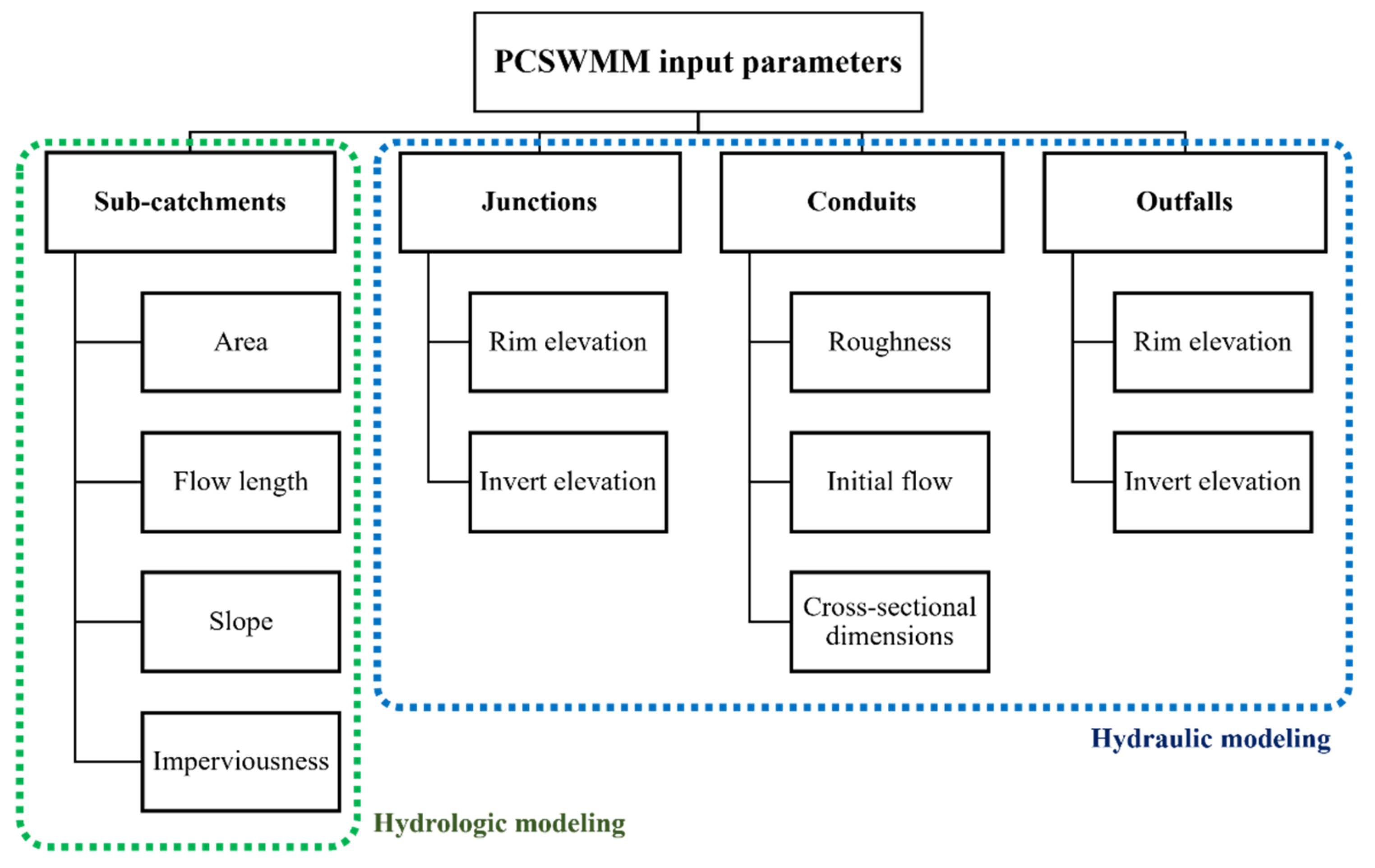
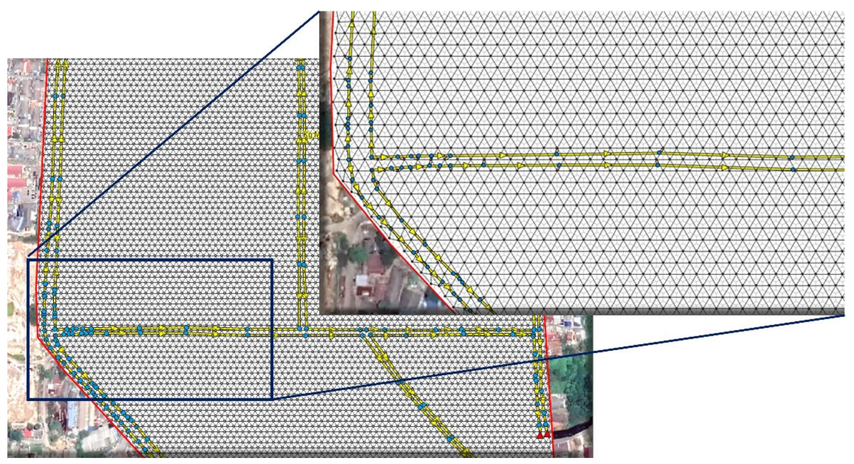
2.3. Model Conceptualization and Parameter Setup

This study used the Computation Hydraulics International (CHI)’s PCSWMM model version 7.3.3095 with the SWMM5 hydrology and hydraulics engine, which is based on the 1-D Saint-Venant equations as follows:

$$\frac{\partial A}{\partial t}+\frac{\partial Q}{\partial x}=0$$

(1)

$$\frac{\partial Q}{\partial t}+\frac{\partial }{\partial x}\left(\frac{Q^2}{A}\right)+gA\frac{\partial H}{\partial x}+gA{S}_f+gA{h}_L=0$$

(2)

where Q, H, and A denote the flow rate, hydraulic head, and cross-sectional area, respectively; $g$ is the gravitational acceleration; $S_f$ is the friction slope; and $h_L$ is the local energy loss per unit length. The continuity and momentum equations (as shown in Equations (1) and (2), respectively) were solved by the finite difference method with successive approximations [38].

Integrated hydrology-hydraulic modeling was carried out to simulate different urban flooding scenarios in the Damansara catchment. Two modules in PCSWMM: rainfall-runoff and flow routing process models, were selected for hydrological and hydraulic modeling, respectively. Figure 2 shows the parameters required for a PCSWMM model. Four input layers, including the sub-catchments, junctions, conduits, and outfalls, play an essential role in the flood simulations. The study area was first divided into sub-catchments using the catchment delineation tool in PCSWMM. For hydrologic analysis, each sub-catchment was assigned with the hydrology input parameters, such as area, flow length, slope, and imperviousness (

Table A1. Hydrology input parameters for the 1-D river flow model.

Name	Area (ha)	Width (m)	Flow Length (m)	Slope (%)	Imperviousness (%)
S1	2024.4916	6952.094	2912.06	1.610	95
S2	700.6339	9060.898	773.25	0.388	90
S3	507.7528	4794.508	1059.03	0.755	40
S4	911.1001	3716.243	2451.67	0.326	40
S5	1315.5053	5953.482	2209.64	0.634	25
S6	714.6110	3105.425	2301.17	0.348	95
S7	1010.6043	11,669.796	866.00	2.080	95
S8	126.5714	3312.347	382.12	0.000	90
S9	331.7123	3658.538	906.68	1.540	95
S10	233.9806	2291.905	1020.90	1.180	95
S11	211.8149	6898.834	307.03	0.326	95
S12	277.4956	2583.782	1073.99	1.300	95
S13	169.6048	7101.189	238.84	0.419	95
S14	55.9358	7649.863	73.12	1.370	95
S15	182.2992	2219.966	821.18	2.070	95
S16	176.0004	2021.669	870.57	0.804	95
S17	352.6336	3034.739	1161.99	0.172	40
S18	422.6794	5633.547	750.29	0.800	95
S19	597.2448	5277.646	1131.65	0.265	95
S20	199.9191	2218.193	901.27	1.220	95
S21	1432.6699	6144.684	2331.56	0.643	50
S22	464.2521	5424.773	855.80	0.000	95
S23	370.3168	6053.797	611.71	0.163	95
S24	133.2000	1395.480	954.51	0.000	95
S25	118.1376	5227.327	226.00	0.000	95
S26	310.2076	3884.539	798.57	0.125	95
S27	378.3916	2934.906	1289.28	0.310	95
S28	82.3326	1545.166	532.84	0.938	40
S29	317.6420	2948.857	1077.17	2.880	95
S30	409.1955	2005.339	2040.53	1.620	50
S31	184.3943	2776.646	664.09	0.000	95
S32	71.9653	10,502.817	68.52	2.920	95
S33	91.6950	1991.638	460.40	0.000	95
S34	198.3507	2080.413	953.42	0.839	95
S35	68.8886	5356.395	128.61	2.330	95

and

Table A2. Hydrology input parameters for the 1-D–2-D drainage overflow model.

Name	Area (ha)	Width (m)	Flow Length (m)	Slope (%)	Imperviousness (%)
S1	3.1546	162.978	193.56	1.550	90
S2	1.9113	180.977	105.61	1.890	50
S3	1.6606	207.679	79.96	5.000	90
S4	5.2218	274.168	190.46	0.525	90
S5	5.2727	270.547	194.89	2.060	90
S6	6.8840	352.375	195.36	1.540	90
S7	7.9970	857.128	93.30	5.460	90
S8	7.5877	1192.472	63.63	2.980	90
S9	7.6306	296.633	257.24	0.777	90
S10	5.9783	261.667	228.47	0.438	90
S11	4.8595	364.444	133.34	0.750	90
S12	3.0559	183.295	166.72	0.600	90
S13	6.3714	344.065	185.18	0.540	90
S14	3.8718	197.098	196.44	0.509	90
S15	3.7131	366.545	101.30	1.970	90

). The impervious percentage for the sub-catchments was taken from the guideline for Urban Stormwater Management Manual for Malaysia (MSMA 2nd Edition) [39], which is in correspondence with the type of land uses. In this study, the Horton infiltration method introduced by Horton [40] was selected, where surface runoff occurs once the rainfall intensities exceed the soil’s infiltration capacity.

The runoff generated from each sub-catchment subsequently enters a junction, usually a manhole structure, exits through a single conduit, representing any water conveyance channel, and finally flows into an outfall point. This process is referred to as hydraulic simulations, in which the dynamic wave method was used in the flood routing model. The required parameters of the rim (surface) and invert elevations for each junction and outfall were assigned based on the Digital Elevation Model (DEM) data, which can be obtained from the United States Geological Survey (USGS) EarthExplorer website (http://earthexplorer.usgs.gov/ (accessed on 7 July 2020)). In the simulation model, junctions and outfalls were connected via conduits (e.g., river or drain in this study). According to MSMA 2nd Edition in 2012 [39], the Manning roughness coefficient for rivers and concrete-lined drains (with a rough finish) were determined as 0.035 and 0.018, respectively. The cross-sectional dimensions for each conduit were based on the surveyed data from several site visits. As for initial flow, it was computed based on Equation (3), derived from the relationship between the average baseflow (Q_B) and catchment area (A) for Peninsular Malaysia [41]:

$$Q_B=0.11A^{0.8589}$$

(3)

3. One-Dimensional River Flow Modeling

For river flow modeling, 35 sub-catchments were created with 205 conduits and 206 junctions, while the river downstream was treated as an outfall, as shown in Figure 3. The rivers were simulated as irregularly shaped conduits, with an initial flow of 7.95 m³/s, computed from Equation (3). An extreme precipitation event in December 2015 was reproduced using the rainfall data (at 5-min intervals) from six rainfall stations within the Damansara catchment, as listed in Table 2. A relatively simple, nearest neighbor-based method [42] was adopted, in which each sub-catchment was assigned rainfall input data from the nearest rainfall station to the sub-catchment’s centroid (Figure A1).

Model calibration and validation should always be undertaken prior to any model application. Among the inferred parameters, the Manning roughness coefficient was selected as the calibration parameter in this study due to its sensitivity to the peak runoff. The Manning roughness of conduits were tested from the initial values of 0.035 to 0.050 (dependent on the river’s surface cover) and adjusted until the optimum values were achieved. The historical December 2015 flood events: 1st–7th and 9th–15th, were chosen for model calibration and validation, respectively. The daily rainfall time series are given in Figure A2. The streamflow data observed at the TTDI Jaya gauging station (No. 3015490) was used to check the water level estimated by the model.

In this study, the simulated peak flows and total flow volumes were satisfactorily predicted with relative errors of less than 10%. The comparison of the observed and modeled water level time series is shown in Figure 4. The previous results from another proprietary software, InfoWorks Integrated Catchment Modeling (ICM) [43], are also presented for comparison purposes in the same plot. In Figure 4, the overall water profiles match well with the observation for both the calibration and validation periods. Variations are expected due to the cross-sectional changes in rivers over the years. It is also noteworthy that both models produce different results. As Pinos and Timbe [44] pointed out, it is likely to be caused by various solution schemes used in solving the governing equations (as in Equations (1) and (2)). In addition to visual observations, some goodness-of-fit measures were adopted to quantify discrepancies between the models and observation, including the coefficient of determination (R²), Nash–Sutcliffe model efficiency coefficient (NSE), and relative error (RE), expressed as:

$$NSE=1-\frac{{{\displaystyle \sum }}_{i=1}^N{\left(h_{obs,i}-h_{sim,i}\right)}^2}{{{\displaystyle \sum }}_{i=1}^N{\left(h_{obs,i}-h_{m,obs}\right)}^2}$$

(4)

$$RE\left(\%\right)=\frac{{{\displaystyle \sum }}_{i=1}^N\left(h_{obs,i}-h_{sim,i}\right)}{{{\displaystyle \sum }}_{i=1}^N{h}_{obs,i}}\times 100$$

(5)

where $h_{obs,i}$ and $h_{sim,i}$ are the ith water level values obtained from the observation and simulation, respectively; and $h_{m,obs}$ is the mean of the observed water levels.

Table 3. Model performance for the calibration and validation periods.

Period	R2		NSE		RE (%)
	PCSWMM	InfoWorks ICM	PCSWMM	InfoWorks ICM	PCSWMM	InfoWorks ICM
Calibration	0.68	0.47	0.52	0.42	4.79	−3.74
Validation	0.62	0.56	0.10	0.26	10.58	9.28

Note: Negative sign means the model overestimates the observed data.

present the model performance in terms of R², NSE, and RE. The calibration performance is confirmed, with R², NSE, and RE values of 0.68, 0.52, and 4.79%. During validation, the results show that the PCSWWM model yields NSE and RE values of 0.10 and 10.58%, respectively. Compared to InfoWorks ICM, higher discrepancies (in terms of NSE and RE) are observed for PCSWMM, which can be explained by the water-level fluctuation observed between 9 and 12 December 2015 (Figure 4b). However, the PCSWMM model still performs satisfactorily in terms of the R² value (0.62) and the reproduction of water level peaks, though some of the peaks are somewhat underestimated.

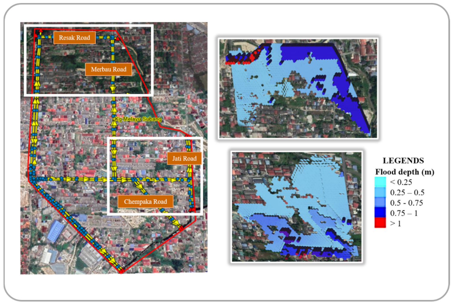
4. One-Dimensional–Two-Dimensional Drainage Overflow Modeling

Considering the computational time for 1-D–2-D simulation, the drainage overflow modeling was only carried out in Kampung Melayu Subang, located in the northern part of the Damansara catchment (Figure 5). This area was chosen due to its frequent floods caused by drainage issues, as reported by DID [8]. In Figure 5, the study area was divided into 15 sub-catchments with 245 junctions, 244 conduits, and 10 outfall nodes. For rainfall input, Kampung Melayu Subang Station (No. 3010001) was assigned as the rain gauge for the sub-catchments. The drains were defined as open rectangular-shaped conduits, representing an open channel with a rectangular cross-section. Based on Equation (3), the initial drainage flow was computed as 0.086 m³/s. There were two scenarios in the hydraulic simulations: scenario 1 (historic drainage) and scenario 2 (current drainage). Note that the current drains in the year 2020 had a width of 0.61–1.37 m and a depth of 0.46–1.52 m, which are on average 15–30% larger than the historic drains in 2015.

In this study, the 1-D–2-D model was constructed using the direct connection approach [45], which allows the 1-D conveyance network (i.e., drainage) to be directly connected to the 2-D floodplain. As the first step in developing a 2-D model, a bounding layer is required to define the extent of the 2-D model domain. In the model setup, a 2-D bounding layer was added with a 10 m resolution hexagonal mesh and a roughness coefficient of 0.033, whereas a point layer or so-called 2-D node layer was generated using the elevation data from the DEM to represent the floodplain topography. Based on the attributes of the layers defined previously, a 2-D mesh layer was finally created with 9416 junctions and 2-D cells. For 1-D–2-D simulation, each junction in the 1-D model was then connected to the closest 2-D junction point, using the connection tool in PCSWMM (Figure 6). This connection allows for the free transfer of flow from the 1-D drainage model to the 2-D model for flood extents in areas.

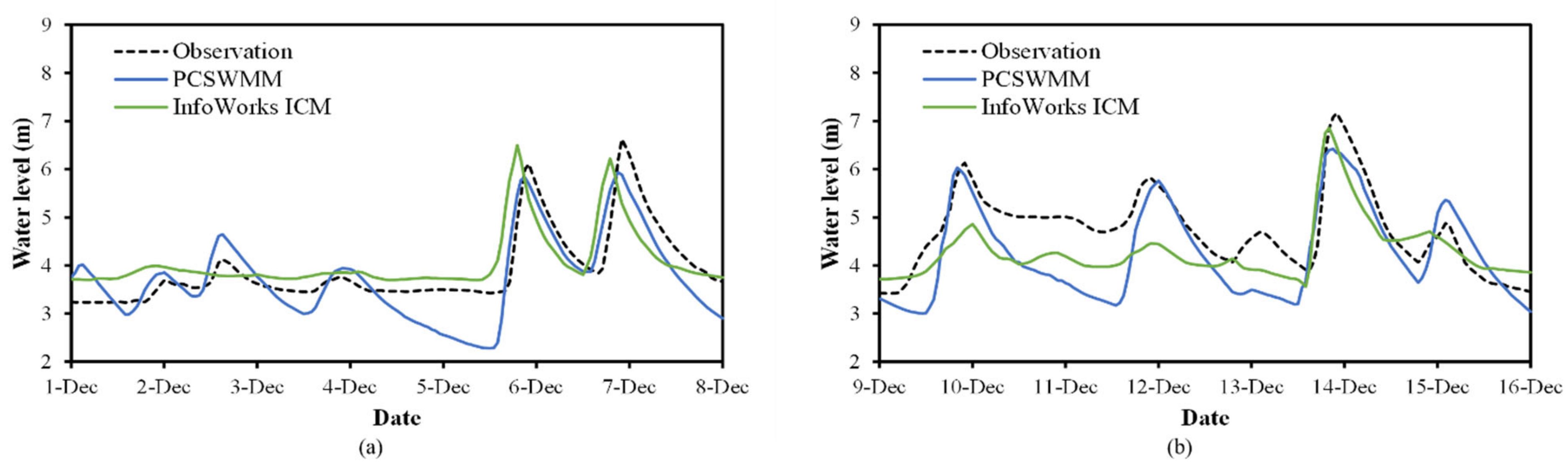
4.1. Comparison of Simulated Data and Observed Data

The scenario of historic drainage overflow was first modeled, referred to as scenario 1, in which the results were used as the reference for validation and comparison. Figure 7 shows the simulation of flooding in Kampung Melayu Subang, displayed in a bird’s eye view via the 3-D viewer in Google Earth Pro. Notably, the simulation corresponds to flooding scenarios in the historic flood event on 31 March 2015. The total precipitation for a 2-h storm duration (05:00 PM–07:00 PM) is 52.2 mm, while the rainfall hyetograph is given in Figure A3.

As shown in Figure 7, flooding typically occurs in the northern and southeastern areas of Kampung Melayu Subang. It is observed that the major affected areas are along Resak Road, Merbau Road, Jati Road, and Chempaka Road, which is in accordance with the previous report showing the flood vulnerability of Kampung Melayu Subang [9]. For a better insight into the flood scenario, the flood depths at the four roads mentioned above are presented in Figure 8. Drainage overflows occur within a few minutes to one hour after the rainfall. The flood depths in the southeastern areas (Jati Road and Chempaka Road) pick up earlier than that in the northern areas (Resak Road and Merbau Road). Unlike the southeastern areas, a gradual increase in flood depth is noticed for the northern areas, until it achieves its maximum depth. The maximum flood depth varies from a minimum of 0.11 m to a maximum of 1.04 m (Figure 8). The results closely match the historical flooding, with maximum depth ranging from 0.3 to 1.0 m [8]. There is a discrepancy in flood depth minima between the simulation and observation, which may be due to the lower grid resolution used in the model, as mentioned by Li and Wong [46].

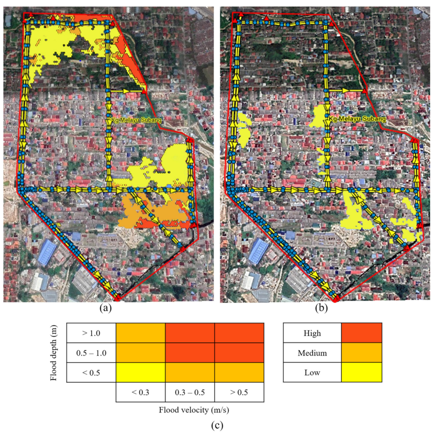
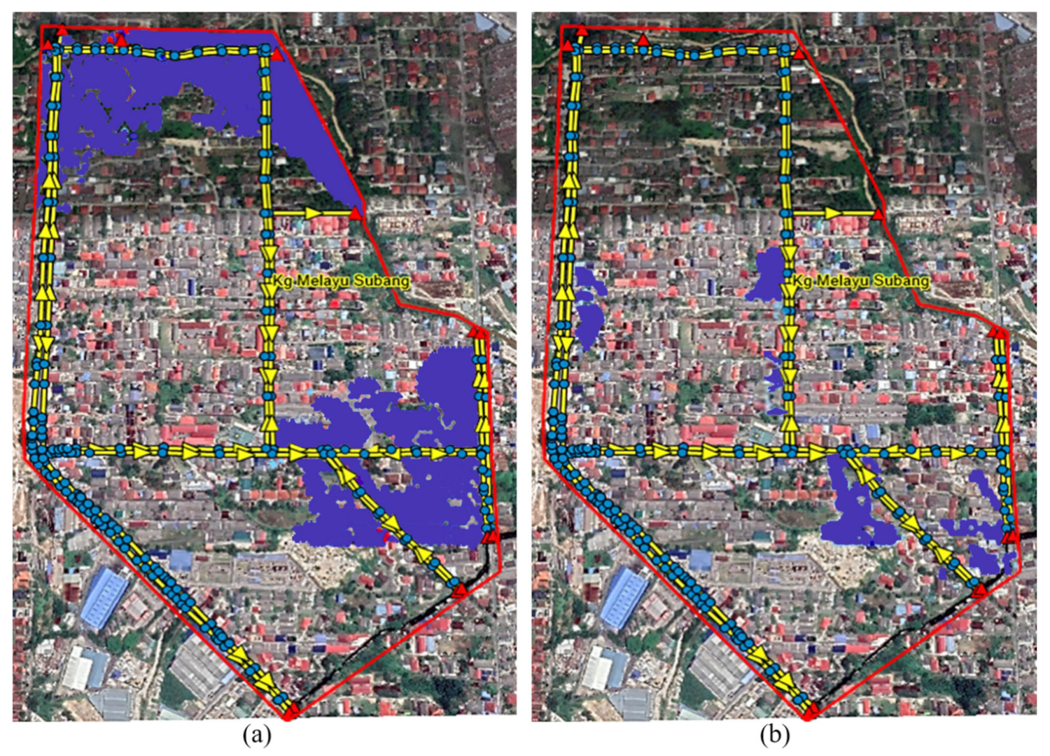
4.2. Comparison between Historical and Current Drainage Scenarios

In this section, the flood inundation results of scenarios 1 and 2 with different sizes of drains are compared in Figure 9. As expected in Figure 9, the flood extent reduces as a result of the increased size of drains in scenario 2. For a 15–30% increase in size for the current drainage, the flood inundation area reduces up to 0.15 km², approximately 78% relative to the historical drainage scenario. This reduction is due to the drainage’s capability to cater to the excess flood flow, thus preventing the drainage overflow, especially in the northern areas of Kampung Melayu Subang. The performance of both models was also evaluated by continuity errors, which are defined as discrepancies in mass balance. The results show that the continuity errors of surface runoff and flow routing are within ±0.1%, thus indicating a satisfactory convergence.

Flood risk mapping plays an important role in floodplain management and acts as a basis for enhancing the awareness and preparedness of citizens. In this study, the flood risk maps were developed for both scenarios 1 and 2 using the flood risk mapping tool in PCSWMM. The flood depth and velocity parameters were used to give the overall flood risk rating as in the flood risk matrix (Figure 10c). Three risk categories can be determined, consisting of low, medium, and high. Note that the range of flood depth and velocity were set based on the maximum and minimum values obtained from the inundation results of scenario 1. Figure 10 shows a comparison between the historical and current drainage scenarios in the flood risk mapping. One can observe in Figure 10a that most of the flooded areas in scenario 1 have low and medium risk; however, high flood risk is spotted at the northeastern and southeastern parts of the study area. For scenario 2, although there is still flooding in the southeastern areas, the entire inundated area is categorized as low risk (Figure 10b), associated with lower flood depth and velocity as compared with that in scenario 1. Overall, the current drain size is sufficient in minimizing the extent of the flooded area and the resulting risk, for the time being at least.

5. Conclusions

The 2015 urban flood events in the Damansara catchment were simulated using the PCSWMM model. The reliability and efficiency of the model were confirmed with the simulations of river flow and drainage overflow. Based on both 1-D and 1-D–2-D flow analysis, the key findings are presented herein:

• In comparison with the observations, the 1-D river flow model presents a relatively satisfactory performance in reproducing the water level peaks. The simulated and observed flow almost varies in the same trend over time, with R², NSE, and RE values of up to 0.68, 0.52, and 4.79%, respectively.
• The 1-D–2-D drainage overflow model excellently performs in predicting the flood-prone areas, as in the historic flood event. Good agreement between the simulation and observation can be seen in the reproduction of the flood depth maxima.
• This work demonstrates the importance of drainage capacity, in which a larger size for the current drainage alleviates floods effectively, leading to a 78% reduction in the flood extent and a change from high to low risk in flood-prone areas.

Globally, there has been an increase in the precipitation frequency and intensity, as reported in the Fifth Assessment Report (AR5) of IPCC [47]. The rainfall-induced hazards, such as urban floods, are expected to increase in the future. Therefore, a detailed investigation and analysis of the catchment’s response to future changes in climate, land use, and urban drainage systems will be included in the next study scopes, using the calibrated and validated PCSWMM model.

References

1. Abedin, S.J.H.; Stephen, H. GIS framework for spatiotemporal mapping of urban flooding. Geosciences 2019, 9, 77. [Google Scholar] [CrossRef] [Green Version]
2. Berndtsson, R.; Becker, P.; Persson, A.; Aspegren, H.; Haghighatafshar, S.; Jönsson, K.; Larsson, R.; Mobini, S.; Mottaghi, M.; Nilsson, J. Drivers of changing urban flood risk: A framework for action. J. Environ. Manag. 2019, 240, 47–56. [Google Scholar] [CrossRef] [PubMed]
3. Kwak, D.; Kim, H.; Han, M. Runoff control potential for design types of low impact development in small developing area using XPSWMM. Procedia Eng. 2016, 154, 1324–1332. [Google Scholar] [CrossRef] [Green Version]
4. Morris, K.I.; Chan, A.; Morris, K.J.K.; Ooi, M.C.; Oozeer, M.Y.; Abakr, Y.A.; Nadzir, M.S.M.; Mohammed, I.Y.; Al-Qrimli, H.F. Impact of urbanization level on the interactions of urban area, the urban climate, and human thermal comfort. Appl. Geogr. 2017, 79, 50–72. [Google Scholar] [CrossRef]
5. Mustaffa, C.S.; Marzuki, N.A.; Khalid, M.S.; Sakdan, M.F.; Sipon, S. Understanding Malaysian Malays communication characteristics in reducing psychological impact on flood victims. J. Komun. Malays. J. Commun. 2018, 34, 20–36. [Google Scholar] [CrossRef] [Green Version]
6. Teng, J.; Jakeman, A.J.; Vaze, J.; Croke, B.F.; Dutta, D.; Kim, S. Flood inundation modelling: A review of methods, recent advances and uncertainty analysis. Environ. Model. Softw. 2017, 90, 201–216. [Google Scholar] [CrossRef]
7. DID. Preparation of Flood Mitigation Master Plan for Sungai Damansara Catchment; Department of Irrigation and Drainage Malaysia: Kuala Lumpur, Malaysia, 2008. [Google Scholar]
8. DID. Ringkasan Laporan Banjir Tahunan Bagi Tahun 2015/2016; Department of Irrigation and Drainage Malaysia: Kuala Lumpur, Malaysia, 2016. [Google Scholar]
9. BNNW. These Are the Flood Hotspots in the Klang Valley. Available online: https://www.brudirect.com/news.php?id=82199 (accessed on 3 January 2021).
10. Metcalf, E. Storm Water Management Model; University of Florida and Water Resources Engineers, Environmental Protection Agency: Washington, DC, USA, 1971. [Google Scholar]
11. Guan, M.; Sillanpää, N.; Koivusalo, H. Modelling and assessment of hydrological changes in a developing urban catchment. Hydrol. Process. 2015, 29, 2880–2894. [Google Scholar] [CrossRef]
12. Jang, S.; Cho, M.; Yoon, J.; Yoon, Y.; Kim, S.; Kim, G.; Kim, L.; Aksoy, H. Using SWMM as a tool for hydrologic impact assessment. Desalination 2007, 212, 344–356. [Google Scholar] [CrossRef]
13. Palla, A.; Gnecco, I. Hydrologic modeling of Low Impact Development systems at the urban catchment scale. J. Hydrol. 2015, 528, 361–368. [Google Scholar] [CrossRef]
14. Yazdi, M.N.; Ketabchy, M.; Sample, D.J.; Scott, D.; Liao, H. An evaluation of HSPF and SWMM for simulating streamflow regimes in an urban watershed. Environ. Model. Softw. 2019, 118, 211–225. [Google Scholar] [CrossRef]
15. Mao, D.; Cherkauer, K.A. Impacts of land-use change on hydrologic responses in the Great Lakes region. J. Hydrol. 2009, 374, 71–82. [Google Scholar] [CrossRef]
16. Sun, N.; Hall, M.; Hong, B.; Zhang, L. Impact of SWMM catchment discretization: Case study in Syracuse, New York. J. Hydrol. Eng. 2014, 19, 223–234. [Google Scholar] [CrossRef]
17. Lee, S.-B.; Yoon, C.-G.; Jung, K.W.; Hwang, H.S. Comparative evaluation of runoff and water quality using HSPF and SWMM. Water Sci. Technol. 2010, 62, 1401–1409. [Google Scholar] [CrossRef] [PubMed]
18. Alamdari, N.; Sample, D.J.; Steinberg, P.; Ross, A.C.; Easton, Z.M. Assessing the effects of climate change on water quantity and quality in an urban watershed using a calibrated stormwater model. Water 2017, 9, 464. [Google Scholar] [CrossRef]
19. Abdul-Aziz, O.I.; Al-Amin, S. Climate, land use and hydrologic sensitivities of stormwater quantity and quality in a complex coastal-urban watershed. Urban Water J. 2016, 13, 302–320. [Google Scholar] [CrossRef]
20. Rai, P.K.; Chahar, B.; Dhanya, C. GIS-based SWMM model for simulating the catchment response to flood events. Hydrol. Res. 2017, 48, 384–394. [Google Scholar] [CrossRef]
21. Yu, H.; Huang, G.; Wu, C. Application of the stormwater management model to a piedmont city: A case study of Jinan City, China. Water Sci. Technol. 2014, 70, 858–864. [Google Scholar] [CrossRef]
22. Wanniarachchi, S.; Wijesekera, N. Using SWMM as a tool for floodplain management in ungauged urban watershed. Eng. J. Inst. Eng. Sri Lanka 2012, 45, 1–8. [Google Scholar] [CrossRef] [Green Version]
23. Bisht, D.S.; Chatterjee, C.; Kalakoti, S.; Upadhyay, P.; Sahoo, M.; Panda, A. Modeling urban floods and drainage using SWMM and MIKE URBAN: A case study. Nat. Hazards 2016, 84, 749–776. [Google Scholar] [CrossRef]
24. Ermalizar, L.M.; Junaidi, A. Flood simulation using EPA SWMM 5.1 on small catchment urban drainage system. MATEC Web Conf. 2018, 229, 04022. [Google Scholar]
25. Paule-Mercado, M.; Lee, B.; Memon, S.; Umer, S.; Salim, I.; Lee, C.-H. Influence of land development on stormwater runoff from a mixed land use and land cover catchment. Sci. Total Environ. 2017, 599, 2142–2155. [Google Scholar] [CrossRef]
26. Yim, S.; Aing, C.; Men, S.; Sovann, C. Applying PCSWMM for stormwater management in the Wat Phnom sub catchment, Phnom Penh, Cambodia. J. Geogr. Environ. Earth Sci. Int. 2016, 5, 1–11. [Google Scholar] [CrossRef]
27. Irvine, K.; Sovann, C.; Suthipong, S.; Kok, S.; Chea, E. Application of PCSWMM to assess wastewater treatment and urban flooding scenarios in Phnom Penh, Cambodia: A tool to support eco-city planning. J. Water Manag. Model. 2015, 23, 1–13. [Google Scholar] [CrossRef]
28. Hamouz, V.; Møller-Pedersen, P.; Muthanna, T.M. Modelling runoff reduction through implementation of green and grey roofs in urban catchments using PCSWMM. Urban Water J. 2020, 17, 813–826. [Google Scholar] [CrossRef]
29. Peng, Z.; Jinyan, K.; Wenbin, P.; Xin, Z.; Yuanbin, C. Effects of Low-Impact Development on Urban Rainfall Runoff under Different Rainfall Characteristics. Pol. J. Environ. Stud. 2019, 28, 771–783. [Google Scholar] [CrossRef]
30. Bhowmick, A.; Irvine, K.; Jindal, R. Mathematical modeling of effluent quality of cha-Am municipality wastewater treatment pond system using PCSWMM. J. Water Manag. Model. 2017, 25, 1–9. [Google Scholar] [CrossRef] [Green Version]
31. Panos, C.L.; Wolfand, J.M.; Hogue, T.S. Assessing resilience of a dual drainage urban system to redevelopment and climate change. J. Hydrol. 2021, 596, 126101. [Google Scholar] [CrossRef]
32. Akhter, M.S.; Hewa, G.A. The use of PCSWMM for assessing the impacts of land use changes on hydrological responses and performance of WSUD in managing the impacts at Myponga catchment, South Australia. Water 2016, 8, 511. [Google Scholar] [CrossRef]
33. Liwanag, F.; Mostrales, D.S.; Ignacio, M.T.T.; Orejudos, J.N. Flood modeling using GIS and PCSWMM. Eng. J. 2018, 22, 279–289. [Google Scholar] [CrossRef]
34. Kumar, S.; Kaushal, D.; Gosain, A. Assessment of Stormwater Drainage Network to Mitigate Urban Flooding Using GIS Compatible PCSWMM Model. In Urbanization Challenges in Emerging Economies: Energy and Water Infrastructure, Transportation Infrastructure, and Planning and Financing; American Society of Civil Engineers: Reston, VA, USA, 2018; pp. 38–46. [Google Scholar]
35. Hasan, H.H.; Mohd Razali, S.F.; Ahmad Zaki, A.Z.I.; Mohamad Hamzah, F. Integrated hydrological-hydraulic model for flood simulation in tropical urban catchment. Sustainability 2019, 11, 6700. [Google Scholar] [CrossRef] [Green Version]
36. Sidek, L.M.; Zaki, A.Z.I.A.; Puad, A.H.M.; Mustaffa, Z. Comparison of Design Flood Hydrograph Using XP-SWMM in Jeluh River, Kajang for Flood Mitigation. In Water Resources Development and Management; Springer: Singapore, 2019; pp. 613–624. [Google Scholar]
37. Searcy, J.; Hardison, C. Double-Mass Curves. Manual of Hydrology: Part I, General Surface Water Techniques; United States Geological Survey: Washington, DC, USA, 1960. [Google Scholar]
38. Rossman, L.A. Storm Water Management Model User’s Manual, Version 5.0; National Risk Management Research Laboratory, Office of Research and Development, US Environmental Protection Agency: Cincinnati, OH, USA, 2010. [Google Scholar]
39. DID. Urban Stormwater Management Manual for Malaysia; Department of Irrigation and Drainage Malaysia: Kuala Lumpur, Malaysia, 2012. [Google Scholar]
40. Horton, R.E. An approach toward a physical interpretation of infiltration–capacity. Soil Sci. Soc. Am. J. 1941, 5, 399–417. [Google Scholar] [CrossRef]
41. DID. Design Flood Hydrograph Estimation for Rural Catchments in Peninsular Malaysia; Department of Irrigation and Drainage Malaysia: Kuala Lumpur, Malaysia, 2018. [Google Scholar]
42. Tiwari, S.; Jha, S.K.; Singh, A. Quantification of node importance in rain gauge network: Influence of temporal resolution and rain gauge density. Sci. Rep. 2020, 10, 9761. [Google Scholar] [CrossRef] [PubMed]
43. Sidek, L.M.; Jaafar, A.S.; Majid, W.H.A.W.A.; Basri, H.; Marufuzzaman, M.; Fared, M.M.; Moon, W.C. High-resolution hydrological-hydraulic modeling of urban floods using InfoWorks ICM. Sustainability 2021, 13, 10259. [Google Scholar] [CrossRef]
44. Pinos, J.; Timbe, L. Performance assessment of two-dimensional hydraulic models for generation of flood inundation maps in mountain river basins. Water Sci. Eng. 2019, 12, 11–18. [Google Scholar] [CrossRef]
45. CHI. PCSWMM Manual; 2292-6062; Computational Hydraulics International: Guelph, ON, Canada, 2018. [Google Scholar]
46. Li, J.; Wong, D.W. Effects of DEM sources on hydrologic applications. Comput. Environ. Urban Syst. 2010, 34, 251–261. [Google Scholar] [CrossRef]
47. IPCC. Climate Change 2014: Synthesis Report. Contribution of Working Groups I, II and III to the Fifth Assessment Report of the Intergovernmental Panel on Climate Change; Intergovernmental Panel on Climate Change: Geneva, Switzerland, 2014. [Google Scholar]
Figure 1. (a) Location of Damansara catchment; (b) distribution of land use in Damansara catchment.
Applsci 11 09300 g001
Figure 2. Input parameters used in PCSWMM for flood simulation.
Applsci 11 09300 g002
Figure 3. Catchment discretization for 1-D river flow modeling.
Applsci 11 09300 g003
Figure 4. Comparison of water level time series modeled and observed at TTDI Jaya: (a) calibration and (b) validation.
Applsci 11 09300 g004
Figure 5. Catchment discretization for 1-D–2-D drainage overflow modeling.
Applsci 11 09300 g005
Figure 6. Direct connections between 2-D mesh (black lines) and 1-D drainage channel (yellow lines).
Applsci 11 09300 g006
Figure 7. Bird’s eye view of simulation results showing flooding in Kampung Melayu Subang.
Applsci 11 09300 g007
Figure 8. Flood depth at different locations in Kampung Melayu Subang.
Applsci 11 09300 g008
Figure 9. Comparison of flood extent between the scenarios with (a) historic drainage in 2015 (scenario 1) and (b) the current drainage in 2020 (scenario 2).
Applsci 11 09300 g009
Figure 10. Flood risk mapping for scenarios with (a) historic drainage in 2015 (scenario 1) and (b) current drainage in 2020 (scenario 2); (c) Depth-velocity matrix used in generating the flood risk maps.
Applsci 11 09300 g010