The Manning’s Roughness Coefficient Calibration Method to Improve Flood Hazard Analysis in the Absence of River Bathymetric Data: Application to the Urban Historical Zamora City Centre in Spain

Featured Application

The methodology proposed in this manuscript makes it possible to improve the estimation of flood zones and their flow depth values in situations where there are no available bathymetric data of the channel (or they are scarce and do not allow for its shape reconstruction). It could improve flood risk assessment too.

Abstract

The accurate estimation of flood risk depends on, among other factors, a correct delineation of the floodable area and its associated hydrodynamic parameters. This characterization becomes fundamental in the flood hazard analyses that are carried out in urban areas. To achieve this objective, it is necessary to have a correct characterization of the topography, both inside the riverbed (bathymetry) and outside it. Outside the riverbed, the LiDAR data led to an important improvement, but not so inside the riverbed. To overcome these deficiencies, different models with simplified bathymetry or modified inflow hydrographs were used. Here, we present a model that is based upon the calibration of the Manning’s n value inside the riverbed. The use of abnormally low Manning’s n values made it possible to reproduce both the extent of the flooded area and the flow depth value within it (outside the riverbed) in an acceptable manner. The reduction in the average error in the flow depth value from 50–75 cm (models without bathymetry and “natural” Manning’s n values) to only about 10 cm (models without bathymetry and “calibrated” Manning’s n values), was propagated towards a reduction in the estimation of direct flood damage, which fell from 25–30% to about 5%.

1. Introduction

Floods are probably the most frequently recurring natural phenomena affecting society (humans and goods) in terms of space and time, regardless of their geographical location or socioeconomic development, as shown by the data collected by the International Disasters Database for the period 1900–2018 (CRED, 2020). This is the main reason why flood risk management has become an essential tool from both a social and economic perspective, with the objective of reducing losses associated with both factors. Furthermore, urban historical centers are characterized by the presence of multiple types of cultural heritage sites, which give it a priceless value upon the consideration of the impossibility of the restoration or recovery of the possible damage caused by natural hazards, in this specific case, by river flooding. This abovementioned duality, but also mainly the irreversibility, of flood damage on cultural heritage (which cannot be reproduced once it has been destroyed) makes the prediction and assessment of the flood risks that may affect these sites a critical task for their preservation. Given this situation, the first natural disaster management strategies that included cultural heritage among its objectives began to be developed in the 1990s. Among these initiatives, one could highlight the “Carta del Rischio” [1], which has been developed by the Italian Central Institute for Restoration since 1992, or the “Noah’s Ark” project of the European Union [2], launched in 2002. At specific sites, only a few works provide applications to case studies at different scales (from regional to local scales) [3,4,5,6,7].

After assessing direct tangible damage (i.e., the direct damage resulting from the physical contact of floodwater with property and its contents), it was found that the economic flood losses have been increasing throughout the past half-century. In the last decade (2008–2018), the economic losses associated with floods exceeded 35 billion USD [8] and, within this period, the flood losses exceeded 19 billion USD in 2012 alone [9,10,11].

The design, sizing, implementation and effectiveness of flood damage mitigation measures require rigorous risk analyses [12]. Within the aspects that a flood risk analysis includes, the greatest technical efforts are usually concentrated on flood hazard assessments. Flood vulnerability analysis is the other determining factor regarding the correct estimation of risk, mainly from the use of magnitude–damage models (e.g., [13,14,15,16,17,18,19]). Since the most common methods of flood hazard analysis are based on hydrological and hydraulic models [20], the greatest uncertainties and sources of error may come from the input data to these models. In the case of hydraulic or hydrodynamic models, the geometry of the channel (topography and bathymetry) [21,22,23,24], the boundary conditions (roughness, flow regime, etc. [25]) and the Manning’s roughness coefficient (e.g., [26,27,28]) are determinants of the goodness of the model and results. In short, the effectiveness of risk mitigation may depend on the correct estimation of parameters such as the roughness of the terrain surface and the detailed bathymetric characterization of the riverbed.

In addition to the key points mentioned above, the urban character of cities’ historical centers must be taken into account. This latter characteristic determines the preferred flow direction of floods inside the urban areas, turning the streets into improvised river channels. To achieve all these objectives, it is essential to have topographic data that are capable of reproducing the geometry and variability of the terrain [22,24,29,30], with the information coming from LiDAR (light detection and ranging) sensors being the most widely used today to derive DEMs (digital elevation models). However, most LiDAR data are not capable of reproducing the river channel morphology due to its inability to penetrate water bodies. Airborne LiDAR sensors (one of the possible sources of LiDAR data) are usually not capable of penetrating water bodies (turbid, turbulent or deep streams and rivers), but they constitute the most common LiDAR data due to their cost-effectiveness for wide areas relative to other LiDAR sources. In fact, as is discussed by Kinzel et al. [31], the available bathymetric LiDAR techniques are usually not designed for shallow waters and are not optimized for providing the spatial resolution necessary for mapping small-to-medium-sized rivers.

However, an accurate representation of river bathymetry (bed topography) plays a critical role in multiple hydrologic and hydraulic applications, including but not limited to flood modelling [23]. To solve these limitations, the acquisition of topographic data through ground surveys and subsequent combination with subaerial LiDAR data may be an efficient solution [32,33,34]. However, this approach has only been used for short river reaches. When the river reach length increases, so do the logistical and cost considerations. Therefore, under the scenario of long river reach study areas, it is common to use alternative methods or models for estimating bathymetry for use in hydraulic or hydrologic analyses. These alternative models assumed a general simplification of river bathymetric geometry, both from the use of simple geometric shapes (triangular, trapezoidal or parabola for a river cross-section) or from other geomorphological and hydraulic methods. The former approach is more frequent [23,35,36,37,38]. From a hydraulic perspective, the horizontally divided channel method (HDCM) was previously used [39,40] to solve the absence of bathymetric data. The HDCM separately considered the flow above and below the bank top and is a better option [39] for dividing the flow than the vertically divided channel method (VDCM) when the floodplain roughness is significantly greater than the channel roughness. When the flow is horizontally divided, the lower part of the flow fits with the bankfull flow (taken from the dominant discharge concept), which has a return period of 1-2 years according to the field observations of Wolman and Miller [41]. However, this bankfull flow return period is dependent on local meteorological characteristics, thus it ranges from about 2 years in the north of Spain to 5 or more years in the southern and southeastern parts of the country. Once the bankfull flow is defined, it is detracted from the inflow hydrograph. In the same way, Chone et al. [40] used LiDAR topography to subtract the flow rate at the LiDAR date from the inflow hydrograph as a solution for the absence of river bathymetric data.

Whatever the proposed methodology, model calibration (when possible) is one of the main tasks that will ensure the quality of the results obtained. To carry out this calibration process, the availability of field data related to the event to be reproduced is essential. When this information is available, model calibration by varying the value of the Manning coefficient is one of the most frequent approaches, which is described by Ardıçlıoğlu and Kuriqui [42]. However, valid information is not always available for the calibration of hydraulic models. This situation is more frequent when we do not try to model a specific event, but rather intend to model a design flow event that has a low frequency of occurrence (high return period). In these cases, and in many others, the lack of available information to calibrate the hydraulic models is compensated by the consideration of a benchmark model against which the results obtained in the rest of the models will be compared [43]. In general, this control model is defined by the availability of more or better data for it.

Several studies have already shown that incorporating bathymetry provides more accurate hydraulic simulations and flooding area estimations, which improve flood hazard analysis at the same time as flood risk assessments. Therefore, the goal of this study was not to reinforce these past findings but to try to open up another approach to improve flood hazard assessment in floodplains, that is, improving flood hazard mapping and main flow variables (flow depth) outside the main river channel (that is, into the flood plains) through the use of calibrated but not “natural” values of Manning’s roughness coefficient. In other words, we looked for a Manning value or range of values that compensated for the effect that the absence of bathymetric data would have on the hydraulic modelling results. This new approach was supported by the assumption that most flood-exposed elements (people and goods) are located out of the river channel and not inside it; therefore, the flow parameters (depth and velocity) in the river channel are not really key points for flood hazard assessment in most cases. Under these assumptions, the use of two LiDAR DEMs (with and without bathymetric data) for the Douro River reach in Zamora city (Spain) allowed us to calibrate a Manning’s roughness coefficient for the main river channel (which is consistent with the value obtained previously from three cross-sections of the river) so that the flooded area and the flow depth in the floodplain converged with the results obtained in the control (or benchmark) model. The hydrodynamic model using the calibrated value show very similar flooded areas, as well as flow parameters (both for the 500-year and 100-year return period peak flows); thus, it can be used for flood hazard and risk assessment. Furthermore, the results of this new approach were compared with results from previous methodological approaches, such as the modified inflow hydrographs. Moreover, the approach proposed here can be replicated for any kind of river and it is cost-saving, as it does not require large ground surveys.

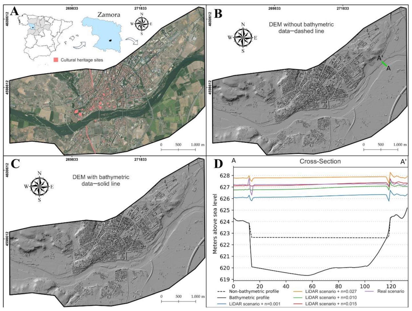
2. Study Area and Data Description

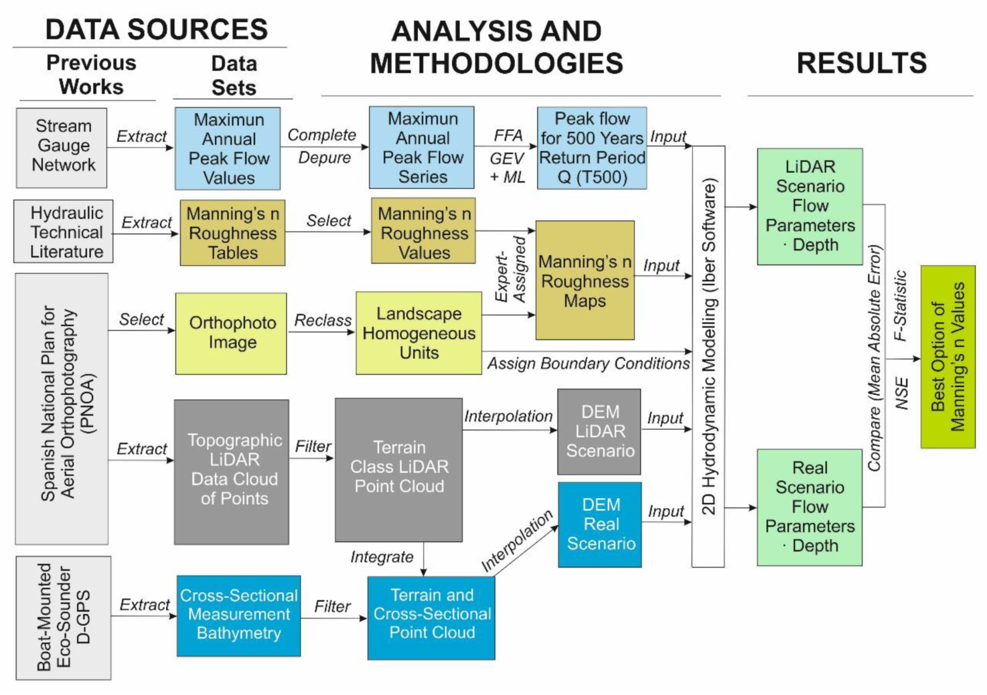
This study focused on comparing the flood area extension over different hydrodynamic models, where Manning’s roughness coefficient was changed in a calibration process. The study area comprises the Douro River reach in Zamora city (Spain), where most of the historical urban center is located on the right side of Douro River, but the urban center located on the left side is developed over lower-lying and flood-prone areas. The Douro River reach in Zamora (Figure 1A) is 7 km long with a mean width of 225 m, and is characterized by a relatively deep, sand-clayey channel with some fully vegetated sandy bars and with several meanders and a flat floodplain.

Topographic LiDAR data [44] are publicly available in the form of point cloud files, which are filtered and classified following the American Society for Photogrammetry and Remote Sensing (ASPRS) standard classification. The vertical accuracy of the LiDAR data used in this study is reported to be lower than 20 cm [44]. The terrain and building types of the LiDAR classification were used to derive the different DEMs. Due to the absence of LiDAR data in the main river channel (since water has low reflectance), it was modelled using a second-order polynomial interpolation of multiple LiDAR cross-sections. Each of these sections presented a height equal to the minimum LiDAR point value and had a length that was restricted to channel boundaries. Although a spline and a third-order polynomial interpolation were tried, the second-order one was chosen because it provided a smooth and downstream-constant slope surface. Bathymetry data were obtained in the form of cross-section measurements that were obtained from boat-mounted echo sounders with D-GPS (differential global positioning system) data acquisition. Both sets of topographic data were combined into a 1 m spatial resolution to create a final DEM (Figure 1C), which was considered to be the “real scenario” (or benchmark scenario). On the other hand, a LiDAR point cloud was also interpolated in the absence of bathymetric data into a 1 m spatial resolution DEM (Figure 1B), which was considered to be the “LiDAR scenario”.

The peak flow values that were used for the hydrodynamic models were obtained from a streamflow gauge at the upstream location of the Douro River reach. A generalized extreme values (GEV) distribution was fitted to the annual maximum flow time series, and the 500-year return period peak flow value (2274 m³ s⁻¹) was selected for our analysis upon the assumption that this value can be considered as a low-frequency or “extraordinary” flood event. To test the efficiency and validity of the proposal, a second peak flow value was selected: in this case, the peak flow value associated with a return period of 100 years (1872 m³ s⁻¹). The reason for not selecting a lower peak flow value, therefore one that was more contrasted with the 500-year return period, was the need for the hydraulic model to include the overflow of the main channel in the flood plain. This need was based on the premise that the usefulness of our proposal is only fulfilled in the floodplain, and therefore, in both cases (different peak flows), the floodplain should be affected.

Finally, PNOA ortho-photographs from 2017 (0.25 m of spatial resolution) were used in combination with a field survey to define the value of Manning’s roughness coefficient (Manning’s n); this map was created for the whole study area at a scale of 1:4.000. It contains ten different roughness units, each of which was assigned a unique Manning’s n according to previously proposed tables [45,46]. For the “real scenario”, a Manning’s roughness coefficient value of 0.027 was assigned for the Douro River’s main channel. All other Manning’s roughness coefficient values related to each terrain surface unit were calculated and were kept constant throughout the calibration process.

3. Methodology

Figure 2 shows the full methodological approach that was used to define the best calibrated Manning’s n value in the river channel, which allowed us to map the flooded area and hydraulic conditions in the absence of bathymetric data.

The entire methodology and analysis that was carried out to obtain the calibrated Manning’s n value that best reproduced (in the absence of bathymetric data) the hydraulic conditions and the flooded area in the floodplain associated with a flood event relative to the benchmark model (availability of bathymetric data) was based on a simple premise: the flow through the channel can be expressed in a simplified form from the following equation:

Q = A ∗ V,

(1)

where Q is the total flow (m³ s⁻¹), A is the cross-sectional area (m²) and V is the mean flow velocity (m s⁻¹).

Starting from this equation, if the absence of bathymetric data meant a decrease in the cross-sectional area of the channel, an increase in the flow velocity of the water in the channel could compensate for the reduction in area and thus allow the flow rate that was circulating through the channel to remain constant. This approach is shown graphically in Figure 3.

3.1. Comparison of Bathymetric Representation

Comparisons of MDE differences and flow depth differences as input and output parameters of the hydrodynamic modelling were carried out. The first of the comparison processes allowed us to quantify the spatially distributed cross-sectional area reduction due to the non-availability of LiDAR data on submerged areas of the main channel. The second one allowed us to spatially assess the distributed differences in flow depth value, as well as to select the optimal model (“LiDAR scenario” plus “best Manning’s n value”) to simulate the flood hazard levels relative to the results of the original, or control, model.

The errors in the bathymetric representation for the “LiDAR scenario” and “real scenario” were compared both using an arithmetic subtraction between the two models (Figure 4A) to obtain a difference value for each pixel of the model and by calculating the mean absolute error (MAE), as shown in Equation (2):

$$\mathrm{MAE}=\frac{{{\displaystyle \sum }}_{\mathrm{i}=1}^{\mathrm{n}}\left|{\mathrm{H}}_{\mathrm{L}}-{\mathrm{H}}_{\mathrm{r}}\right|}{{\mathrm{n}}_{\mathrm{c}}}$$

(2)

where H_L is the elevation of the ith cell for the “LiDAR scenario” DEM, H_r is the elevation of the ith cell for the “real scenario” DEM and n_c is the number of cells used for the analysis.

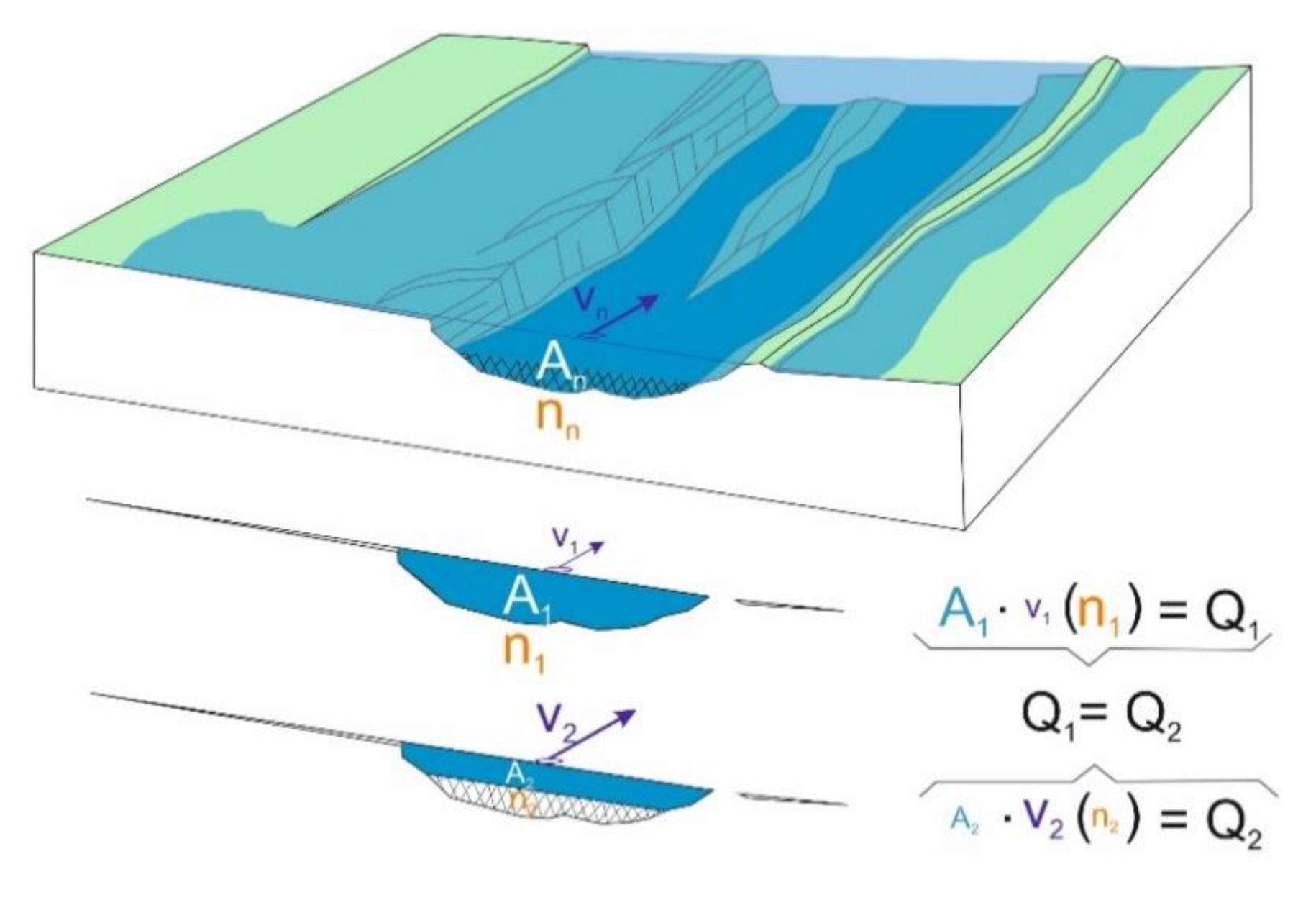
3.2. Hydraulic Modelling and Calibration Process

The hydrodynamic modelling for all configurations was performed using 2D Iber software [47], which is a two-dimensional mathematical unsteady flow model that is used to simulate the free surface flow in rivers and estuaries and employs a high-resolution finite volume as a numerical method to solve the depth-averaged 2D shallow water equations, also known as Saint Venant equations. Iber software requires a geometric description of the channel in the form of a 3D mesh for performing hydraulic computations. Only the hydraulic modelling of peak flows was carried out, as these peak flows were related to maximum flooded area extension.

The calibration process was carried out in a similar way to a sensitivity analysis of the hydrodynamic model to changes in the Manning’s n parameter. The extreme values of the Manning’s n for the Duero riverbed were, on the one hand, a minimum value of 0.001, and on the other hand, a maximum value of 0.027 (similar to the value used in the “real scenario”). No higher values of the Manning’s n were considered on the basis that, with the same value of surface roughness parameter and a decrease in the cross-sectional area of the channel (due to the absence of bathymetric data in the “LiDAR scenario”), both the flooded area and the flow depth values should be clearly higher than the one obtained in the “real scenario”, which here was considered the benchmark model. To complement and complete the analysis, two other scenarios were considered for comparison with the control model. On the one hand, a model with a variable and spatially distributed Manning’s n value was considered (which was obtained from the previous models using the Manning’s n value that showed the best fit for each of the pixels within the river channel, as is shown in Figure 5). Second, the HDCM model, as applied by Chone et al. [40], was considered by subtracting the flow value at the date of acquisition of the LiDAR topography from the peak flow value of the 500- and 100-year return period.

As the present approach is only useful for floodplain areas and not for river channels, the data collected for the calibration process were located in the Douro river floodplain. The results of different Manning’s n values inside the river channel were also compared to the benchmark model to achieve a spatially distributed Manning model where Manning’s n value inside the river channel varied for each model cell. Manning’s n value is dependent on which model (with a constant value of Manning within the channel) performed best in the comparison against the control (or benchmark) model.

3.3. Comparison of Hydrodynamic Model Outputs

To evaluate the suitability of the different hydrodynamic models that were generated in the calibration process, the flow depth parameter was selected since it was the most commonly used parameter for flood risk analysis through magnitude–damage models as a flood vulnerability approach. The hydraulic outputs (flow depth) generated by the Iber software were exported into geo-referenced ASCII raster files (*.asc files) for each of the “LiDAR scenario + Manning’s n value” models, and further outputs were compared to the benchmark model generated using the “real scenario” topography in the GIS software ESRI^® ArcGIS 10.6.1. Spatially distributed flow depth differences between calibrated models and the control model, as well as random sample creation and geo-statistical analysis input parameter calculations, were also generated inside the ESRI^® ArcGIS environment.

The analysis of different results started with descriptive statistics of the flow depth value differences between the “LiDAR scenario” models (with different Manning’s n values) and the “real scenario” in the set of random samples (nearly 7000 random points for the 500-year return period peak flow and around 3600 random points for the 100-year return period). The mean, median, mode, standard deviation, variance and Nash–Sutcliffe efficiency index were calculated and compared for analysis purposes. Box plots were used to explore the spatial distribution behavior of different levels of depth errors. First, error location points were classified depending on the distance to the river bank with classes of 100 m width. Then, a boxplot was graphed for each spatial class. Distance bands to the river were computed using the Near ArcMap tool [48]. The Matplotlib library [49] from Phyton software was used to perform a descriptive and graphical statistical analysis.

The Nash–Sutcliffe efficiency (NSE) index was used as given in Equation (3):

$$\mathrm{NSE}=1-\frac{{{\displaystyle \sum }}_{\mathrm{i}=1}^{\mathrm{n}}{\left({\mathrm{D}}_{\mathrm{m}}-{\mathrm{D}}_{\mathrm{o}}\right)}^2}{{{\displaystyle \sum }}_{\mathrm{i}=1}^{\mathrm{n}}{\left({\mathrm{D}}_{\mathrm{o}}-{\overline{\mathrm{D}}}_{\mathrm{o}}\right)}^2}$$

(3)

where D_m is the flow depth value of the modelled “LiDAR scenario”, D_o is the flow depth value in the “real scenario” and ${\overline{\mathrm{D}}}_{\mathrm{o}}$ is the mean flow depth value for the “real scenario”.

Furthermore, the flood inundation extent that resulted from each calibrated Manning’s n model was also compared with the “real scenario” model using the F-statistic, as given in Equation (4):

$$F statistic=\frac{A_{Lr}}{A_L+A_r-A_{Lr}}\times 100$$

(4)

where A_L is the observed inundation area (inundation area of the reference model in this case, “real scenario”), A_r is the modelled inundation area (“LiDAR scenario”) and A_Lr is the area that is common to both the “real scenario” and the “LiDAR scenario” inundation maps.

The F-statistic index, which was previously used in [23,29,50,51,52], allowed us to compare floods throughout the inundation extent resulting from each hydrodynamic model, where the hydrodynamic models differed was in the bathymetry data (as previously used) or in the Manning’s n value at the main river reach (as was used here). A value of 100 meant a perfect match between the observed and predicted areas of inundation, and a lower F indicated a discrepancy between the two.

4. Results and Discussion

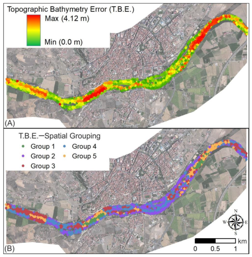
4.1. “Real Scenario” vs. “LiDAR Scenario” Bathymetric Differences

The use of the MAE index on a random sample of 3000 points (located in the river channel, independent of the samples obtained in the floodplain) made it possible to estimate the error in the bathymetry data between the “real scenario” and the “LiDAR scenario”. The MAE index adopted a value of 1.57 m. This was not surprising if we consider the type of riverbed that the Douro River had in the study area under analysis. However, when transferring the MAE index value to the average width of the river’s cross-section, we obtained a reduction in the cross-sectional area of 353.25 m². This reduction in the cross-section could cause a reduction in the flow capacity of the channel of 353.25–529.87 m³ s⁻¹ at times when the flow was medium–low and its average speed could be considered to be between 1–1.5 m s⁻¹. At times of flooding, when the average speed of the water could rise to values of 3 m s⁻¹ or more, the reduction in the flow capacity in the channel could rise to values of 1059 m³ s⁻¹ or even more.

The absolute error in bathymetric data between the “real scenario” and the “LiDAR scenario” ranged from 0–4.115 m at the Douro River reach, and it showed a clear trend from the river banks to its centerline (Figure 4A). At the same time, a more irregular pattern was observed in the downstream direction, where the application of a grouping analysis over the spatial distribution of errors in bathymetry did not show clear trends when no spatial constraints were used (compare with spatial constraints, such as K-nearest neighbors or Delaunay triangulation techniques, which show artificial grouping due to the requirements of spatial constraints between points in the same group). When no spatial constraints were used, the grouping of the random sample points could be related to the “riffle and pools” longitudinal profile shape (Figure 4B) of natural rivers.

All previous data pointed out the importance of bathymetric data for the correct hydrodynamic modelling of the flow event flooding area, as well as the uncertainty of flood parameter results when using LiDAR data without a bathymetric data improvement. In this sense, Cook and Merwade [29] previously pointed out this problem when they showed a reduction of between 5 and 20% in flooded areas when bathymetric data were combined with LiDAR data, with this reduction range being based on the channel type and hydrodynamic model (1D or 2D). In the same way, Saleh et al. [53] highlight that, in the context of determining water levels at a specific location, the difference in bathymetry could be very important. Furthermore, they also noted how this difference may be more evident when we use DEMs or remote sensing techniques to identify river geometry at the regional scale since it is difficult to obtain an accurate bathymetric river representation. Other assessments [23] pointed towards the same conclusion, but there is no quantification of the dependence between bathymetric errors and flooded area differences.

4.2. Manning’s n Value Calibration

The Manning’s n value calibration process was carried out first for the 500-year return period peak flow, and it was done in two steps. First, focusing on a cost-saving approach that would allow its application in places with very different socio-economic development, the calibration was carried out based on the results obtained in a series of cross-sections of the Douro River. At the location of each cross-section, a hydrodynamic model was generated and a best fit Manning’s n value model was defined (Figure 1D). A non-homogeneous Manning’s n value for each cross-section was found, which pointed towards the assumed hydrodynamic simplification when we use a homogeneous surface roughness coefficient for the whole river reach. This point is discussed later.

From the different best fit Manning’s n values of each cross-section, a mean value of n = 0.015 was obtained. However, given the non-homogeneous results obtained in the previous step, a second calibration phase was carried out.

In this second phase, the hydrodynamic model was extended throughout the study area. The latter aspect favored the achievement of multiple objectives, such as the rapid comparison of results in the location of the river cross-sections that were used in the first calibration phase. However, it also allowed for statistical and geostatistical analyses of the results to be carried out to achieve a better understanding of them in such a way that one could finally obtain a selection, based on scientific criteria, of the hydrodynamic model based on the “LiDAR scenario” topography and the best value (or range of values) of Manning’s n coefficient.

As a complement to the above, the results obtained from two other models were analyzed. On the one hand, use was made of a model that presented a variable spatial distribution in the value of the roughness coefficient in the channel (obtained from the roughness values that offered a better adjustment relative to the control model, i.e., the “real scenario”, for each point in the channel). On the other hand, a model with a roughness coefficient value of 0.027 was considered (similar to the control model), albeit with a reduced peak flow value (from 2274 to 2114 m³ s⁻¹) depending on the measured flow rate at the date of acquisition of the LiDAR data.

The calibration, optimization and validation of the parameters in the models require having observational elements of calibration, such as the existence of a gauging station with its available stage–discharge curve in the case of the hydraulic models [54,55]; the existence of stage water plaques of historical floods with a known peak flow value; or other types of high-water marks, such as paleo-hydrological evidence (slackwater deposits or dendro-geomorphological floods [56]). In addition, it is not sufficient to have a single element for calibration because different combinations of parameters can give convergent results at one point; rather, multiple points are needed to adjust them, and these are not always available [28]. In fact, as pointed out by Hawker et al. [43], the availability of observational elements of calibration is not possible in many cases.

However, the readjustment of compensation between parameters, which is the strategy followed in this work, made it possible to compensate for the deficiencies in bathymetry by readjusting the roughness in a relatively simple way that was applicable to any section or situation, whether or not there were calibration elements.

In short, the methodological approach adopted, although it can be complemented with other approaches, is an innovative strategy that can substantially improve hydrodynamic models, hazard analyses, risk assessments and, finally, the effectiveness of flood risk mitigation measures. Evidently, this was all done in places where there was no bathymetric information and where such information could not be obtained, and only for the floodplain, not for the river channel.

4.3. Flow Depth Models Analysis and Optimal Model Selection

The hydrodynamic output parameter of flow depth, which was derived from each Manning’s n value calibration model that was constructed upon the topography of the “LiDAR scenario” model, was compared to the control model, i.e., the so-called “real scenario”. First, the global results were analyzed both as flow depth differences and as flood area extensions by using descriptive statistics parameters, such as mean, median, variance or standard deviation, and with the use of the Nash–Sutcliffe efficiency index and the F-statistic index. All these statistical indexes are shown in

Table 1. Statistical data about Manning’s n value calibration process, considering both hydrodynamic outputs, namely, flow depth and flooding area.

	Mean	Median	Mode	Standard Deviation	Variance	F-Statistic	NSE Index
LiDAR Scenario + n = 0.001	0.231	0.417	0.100	−0.110	0.174	81.76	0.9976
LiDAR Scenario + n = 0.010	0.024	0.326	0.026	0.050	0.106	91.94	0.9998
LiDAR Scenario + n = 0.011	0.000	0.311	0.010	0.050	0.096	92.30	0.9976
LiDAR Scenario + n = 0.012	−0.029	0.298	−0.007	0.050	0.089	92.68	0.9860
LiDAR Scenario + n = 0.013	−0.061	0.287	−0.027	0.050	0.082	93.19	0.9944
LiDAR Scenario + n = 0.014	−0.094	0.280	−0.045	0.050	0.079	93.46	0.9727
LiDAR Scenario + n = 0.015	−0.130	−0.073	0.030	0.269	0.073	93.92	0.9994
LiDAR Scenario + n = 0.016	−0.169	−0.106	0.040	0.263	0.069	93.34	0.9985
LiDAR Scenario + n = 0.018	−0.251	0.257	−0.191	−0.182	0.066	91.11	0.9953
LiDAR Scenario + n = 0.020	−0.332	0.254	−0.314	−0.312	0.065	89.10	0.9920
LiDAR Scenario + n = 0.027	−0.641	0.260	−0.660	−0.750	0.068	84.19	0.9236
LiDAR Scenario + ndistrib	0.010	0.005	0.050	0.316	0.100	93.05	0.9981
real Scenario + Q reduced + n = 0.027	−0.393	−0.407	−0.416	0.258	0.067	87.65	0.9894

.

From the analysis of the simulation points as a function of the flow depth values, it was found that the differences between the “real scenario” and the “LiDAR scenario (Manning’s n value = 0.011)” had the lowest mean deviation, with a perfect average fit (0.000); the lowest median deviation results were found for the “LiDAR scenario (spatially distributed Manning’s n value)”, which slightly underestimated the flow depth (0.005); the lowest mode value was related to the scenario with Manning’s n value equal to 0.012; the variance of the deviation had a random behavior.

The Nash–Sutcliffe efficiency index was calculated as one minus the ratio of the error variance of the modelled hydrodynamic output divided by the variance of the observed hydrodynamic output. In our assessment, the output was the flow depth parameter.

The NSE index showed very similar values for almost all of the hydrodynamic models. The best value was associated with the hydrodynamic model with a Manning’s n value of 0.010, but the differences relative to other models (like models with n = 0.015, 0.016 or a spatially distributed n value) were not significant. All models showed high values of the NSE; therefore, the error variance of the modelled hydrodynamic outputs was much lower than the actual variance of the “real scenario” hydrodynamic model flow depth parameter. From the results of the NSE index, it was difficult to make the selection of the best Manning’s calibrated hydrodynamic model.

Just as the results of the flow depth parameter given by the NSE index were not fully significant to select the best calibrated hydrodynamic model option, the results from the F-statistic index (Table 1) produced the same result. The F-statistic index showed many close values for the hydrodynamic models, with Manning’s n value ranging from 0.010 to 0.018 (always above a value of 90), with the best value of the F-statistic index linked to the Manning’s n value of 0.015. The F-statistic improvement from Manning’s n value of 0.010 to 0.015 was only about 1.5%.

As a conclusion, we could say that the analysis of the flow depth results from all calibrated models not giving us a strong criterion for the better option selection means that all models using Manning’s n values ranging from 0.010 to 0.016 may be suitable to reproduce the conditions shown by the control model, i.e., the “real scenario” hydrodynamic model. The results shown by these models were similar in quality to those obtained by the use of the variable and spatially distributed Manning n value model, and they were better than the result shown by the HDCM approach. Based on the results obtained up to this point, a second phase of flow depth values analysis was necessary and a geo-statistical approach was carried out, where the distance to the main river channel was taken into account for the flow depth analysis.

When the results were analyzed as a function of the distance to the riverbanks (Figure 6), less deviation was also observed for the LiDAR scenario models with Manning’s n values ranging from 0.011 to 0.015 (the model with an n value of 0.016 began to show a slight deviation towards flow depth overestimation). From the best-calibrated models, those linked to a Manning’s n value equal to 0.013 or 0.014 probably showed the lowest dispersion against the zero error line.

If the analysis of flow depth values was carried out in intervals of distance from the riverbanks (Figure 7), the scenarios that best adjusted the intervals of maximum–minimum deviation were also those ranging from Manning’s n value equal to 0.010 to 0.014. The “LiDAR scenario (Manning’s n value = 0.010)” showed the best results for shorter distances from the riverbank, with a very good fit for distances from 0 to 150 m. The “LiDAR scenario (Manning’s n value = 0.012)” gave the best results for distances from 150–300 m off the riverbank. Moreover, the “LiDAR scenario (Manning’s n value = 0.013)” showed a good fit for all distances up to 300 m. However, for distances over 300 m, the “LiDAR scenario (Manning’s n value = 0.014)” probably showed the best fit from the range of different Manning’s n values calibrated. For this model, most of the error in the flow depth value lay within an interval of ± 10–12 cm, although this error increased to 15–20 cm when we got close to the riverbank. All these models substantially improved the results obtained in the model in which the natural value of Manning’s parameter n was maintained.

When we analyzed the results that were associated with the spatially distributed Manning’s parameter n model and those associated with the HDCM model, we observed that in both cases, the results were better than those associated with the model that preserved the natural value of Manning’s n parameter. However, in neither case did the results approach the best of the models with a constant and calibrated Manning’s n value. Thus, the HDCM model was one of the worst performers in this study. The bad performance of the HDCM model may have been due to the large difference between flow rates on the date of the LiDAR data and the 500-year return period peak flow, as well as the likely significant differences in flow velocity in each case, where the higher flow velocities would require less of a channel cross-sectional area (Figure 3). On the other hand, the model with a spatially distributed Manning’s n value provided a very good fit with the control model (“real scenario”) of up to about 500 m distance from the channel; however, at further distances, it underestimated the flow depth more than the models with a constant Manning’s n parameter and values between 0.013 and 0.015. Therefore, if the risk is to be assessed at a short distance because this is where the exposed and vulnerable elements are located (farms, transport infrastructure, etc.), the scenario “LiDAR scenario (Manning’s n value = 0.011)” or the spatial distributed Manning’s n value model are of interest, while if risk analysis is to be carried out for elements distant from the riverbed (homes and towns far from the river but within a flood zone), the scenario “LiDAR scenario (Manning’s n value = 0.012 to 0.015)” can be used. This gives rise to an interesting discussion on the need to use different roughness indices depending on the flow rate and its return period, as some authors have already pointed out (but in the opposite direction to these results [55]). This variation in the parameters and indices to be used in hydrological and hydraulic models depending on the magnitude of the event has already been described extensively in the scientific-technical literature for other parameters, such as initial abstractions (curve number) as a function of precipitation intensity.

The coefficient of water bottom friction was investigated extensively and is known to depend on the particle sizes of materials on the river bed. There have been many studies on friction parameter estimation, especially on a relationship between estimated Manning’s coefficients and river bed conditions. These range from the classical tables and lists [57,58], to present-day estimations using fractals and connectivity [59,60] from remote sensing information [61], as well as including visual guides [45] and technical determination procedures [62,63]; all of these methods can be grouped in two kinds of approaches: (i) grain size–roughness relationships for different river bottom patches or polygons and (ii) micro-topographical analyses of bathymetrical data.

The first group is used in technical reports and studies of large river reaches for hydrodynamic modelling and civil engineering; the second group is usual in scientific detailed studies of small river channels for geomorphological and ecological analysis. Both approaches are necessary and complementary because they depend on the scale and objectives of roughness estimation. However, it is very important to quantify predictive uncertainty in the hydrodynamic modelling of shallow water flow in response to uncertainty in friction parameterization [64].

However, in any case, a fully spatially distributed Manning’s coefficient based upon the physical characteristics of terrain (mainly the riverbed characteristics) was not achieved due to the complex distribution and the high degree of spatial variability in the physical characteristics of the terrain (grain-size and micro-topography distributions) and vegetation. This objective is already feasible for floodplains [61] by using UAVs, but not for the submerged areas of river channels.

Based on the whole scope of the results of our analysis, the use of a spatially distributed Manning’s n value became necessary. Manning’s n value is usually calibrated within a river reach using a uniform value for all reaches, although the use of non-uniform values was pointed out by previous studies [65] that used a different Manning’s n value for each river reach at the Lower Tapi River (India) to get the best-fit calibrated HEC-RAS model. In this sense, Attari and Hosseini [66] showed a methodological framework for the automatic river segmentation into different river reaches that were fitted with a non-uniform Manning’s n value. Both approaches were utilized prior to the use of a non-uniform value for the roughness coefficient along a sequential river reach segmentation, but they did not use a real spatially distributed Manning’s n value. Although a more complete study of spatially distributed values of Manning’s n parameter would be necessary and convenient, the approximation to its use that was carried out in the present study did not show significantly better results than those of the other models considered.

In our methodological approach, we used the 500-year return period peak flow to develop the methodological framework, while the 100-year return period peak flow was used as the test model. The statistical results of the test model (Table S1 in Supplementary Materials) showed a slight difference from the 500-year return period peak flow model. A similar dependence on the statistic used was observed relative to the hydraulic model, which offered better results compared to the control model. The geostatistical analysis of results for the test model, considering the distance from the riverbank, showed very similar trends (Figures S1 and S2) to those related to the 500-year return period. Therefore, the scatter plot of Figure S1 shows that the best fit with the control (or benchmark) model was linked to Manning’s n value in the range of 0.014–0.016. The results of the box plot (Figure S2), which were the same as for 500-year return period models, showed differences in the best fit that was linked to the distance to the riverbank. As discussed above, the best fit for shorter distances was obtained with a lower Manning’s n value (about 0.011), while for distances equal to or greater than 500 m, the model that offered the best results was possibly the one with a Manning’s n value of 0.016. As for the 500-year return period, the test model linked to the HDCM approach showed an overestimation of the flow depth values for all distances to the riverbank. For all hydraulic models related to the 100-year return period, an increase in uncertainty could be observed at further distances from the riverbank, which was due to the smaller flooding area at the floodplain (and the consequent lower number of sample points at further distances) than the one related to the 500-year return period models.

In general, we observed that the best-fitting Manning’s n value increased slightly from the methodological developed model (500-year return period peak flow) to the methodological test model (100-year return period peak flow). However, taking this into account, the optimal range of Manning’s n value from 0.014 to 0.016 could be defined. Within this range of Manning’s n value, the flow depth errors in the river floodplain were drastically reduced from the model without bathymetry data and a “normal” (0.027 in the study site) Manning’s n value.

The results from the two peak flows considered in the present assessment point towards the validation of our methodological approach, and the usefulness of using a calibrated and reduced values of Manning’s n coefficient where the topography of the riverbed is not available and its acquisition lies outside the economic budget of flood risk managers.

4.4. Local Results at Cultural Heritage Sites in Zamora (Spain)

Beyond the results of the overall study area (with or without riverbank distance dependence), some control points (Figure 8) that are linked to different housing types in Zamora city were used for the result quality analysis of the Manning’s-n-value-calibrated models. Four control points were selected, representing different types of buildings in the vicinity of the city of Zamora. Checkpoints 1 and 3 represented buildings in an urban environment with a high building density, checkpoint 2 corresponded to a cultural heritage site (chapel) and, finally, checkpoint 4 corresponded to a house that was isolated among agricultural fields.

In all cases, the absence of bathymetric data in the peak flow hydraulic modelling implied a flow depth overestimation ranging from 50 to 75 cm, where no process of artificial modification of the Manning’s n value (calibrated model with n = 0.027) was carried out. These flow depth errors could be drastically reduced through the Manning’s n value calibration process, as shown in Figure 8. However, as was also observed previously, the results obtained at the four control points did not show complete homogeneity. Again, the range of values between 0.010 and 0.014 seemed to show the best results overall. However, depending on the spatial location of the control point, it was observed that values lower than 0.010 could also give optimal results, but values higher than 0.014 did not. The selection of only four locations may not be representative for the whole study area, and the previously exposed results (where the best fit was obtained for the Manning’s n value ranging between 0.014 to 0.016) had greater confidence, but they were illustrative of the overestimation of flow depth in the absence of bathymetric data without some kind of calibration process.

By transferring these differences in flow depth to the analysis of direct economic damage caused by floods, they can lead to significant differences in damage estimates. Thus, based on a widely used magnitude–damage model [15], we found that a difference in the flow depth of 50–75 cm could lead to a variation in the direct damage estimates of 25–30%. From the same model, we could estimate that, if we associated an average error of 10 cm with the calibrated model with n = 0.014, the error in the damage estimate would be around 6%. These percentages of economic direct damage can vary depending on the non-linearity of the distribution of flood damage associated with the flow depth value, as well as the damage model used. Wagenaar et al. [67] pointed out that the resulting uncertainties in estimated damage (due to different models) are in the order of magnitude of a factor of 2 to 5.

Furthermore, from the results obtained, it can be seen that the use of a reduced or lower (relative to that which is naturally associated with the characteristics of the riverbed) Manning’s n value between 0.011 and 0.016 could lead to an error in the estimation of the flow depth that was no more than 25 cm, which, transferred to the estimation of direct damage, meant an approximate damage value error of 12%. Therefore, the use of an artificially lower Manning’s n value could reduce the error in estimating flood damage by half. Therefore, this can be an interesting starting point for the improvement of flood damage estimates in areas without bathymetric data availability (even taking into account the fact that obtaining bathymetric data will always be the best option to achieve the best results). Furthermore, it could serve to carry out hazard analyses and, therefore, more personalized risk analyses depending on the elements at risk to be analyzed and their distances from the riverbanks.

However, from a practical point of view, this would introduce complexity into the systematic production of hazard and risk mapping, such as those of FEMA [68] in the USA, SNCZI [69] in Spain, or the Flood Factor [70], also in the USA. At the same time, it would give dynamism and ease of updating to large-scale local studies, which are optimal for urban areas or vulnerable infrastructures (large dams, nuclear power stations, industrial complexes, etc.).

5. Conclusions

The present manuscript shows a new approach for improving flood hazard maps where bathymetric data are not available (or they are scarce, such as a few cross-sections for the whole river reach). The proposed solution to this unavailability of bathymetric data is valid for river floodplains but not inside the river main channel. Unlike the approaches based on the generation of simplified bathymetric shapes, or the hydraulic corrections (HDCM model), the proposal of this manuscript was based on the calibration of the Manning’s n value (roughness surface index). This calibration point toward the use of abnormally low values for a natural channel sought to compensate for the reduction in the channel cross-section area using an increase of the flow velocity in the channel itself. The main conclusions that can be derived from this study are as follows:

-

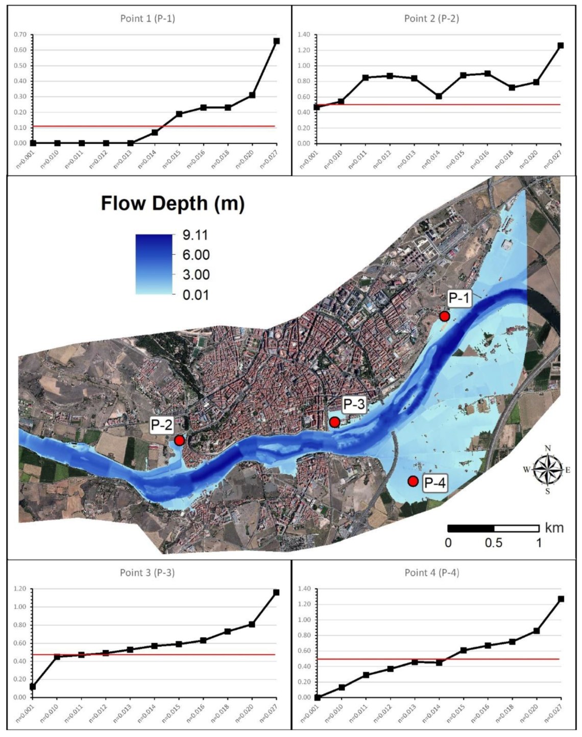
The results obtained show a clear improvement when compared to the direct use of LiDAR topographic information combined with a Manning’s n value according to the characteristics of the river channel studied. The results from the methodological developed model (500-year return period peak flow) and the methodological testing model (100-year return period peak flow) converged toward a range of Manning’s n values from 0.014 to 0.016, which is far from the 0.027 that is selected based on the Douro River reach characteristics. A slight uncertainty in the best range of the Manning’s n value was seen depending on the magnitude of the peak flow rate used. The magnitude of the peak flow rate and the optimal Manning’s value show an inverse relationship.

-

For the case of the Douro River in Zamora, the results of the hydrodynamic modelling under the “LiDAR scenario” and the “natural” Manning’s n value conditions (n = 0.027) caused average errors of 50–75 cm in the flow depth estimation. By calibrating the Manning’s n value, these average errors could be reduced to a value close to 10 cm.

-

By transferring the errors in flow depth to the estimation of direct damage due to floods (based on the widely used USACE damage magnitude model), we achieved a reduction in the error in the percentage of damage from values of 25–30% to errors close to 5%.

-

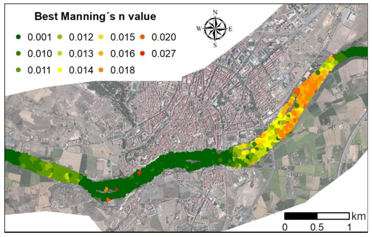
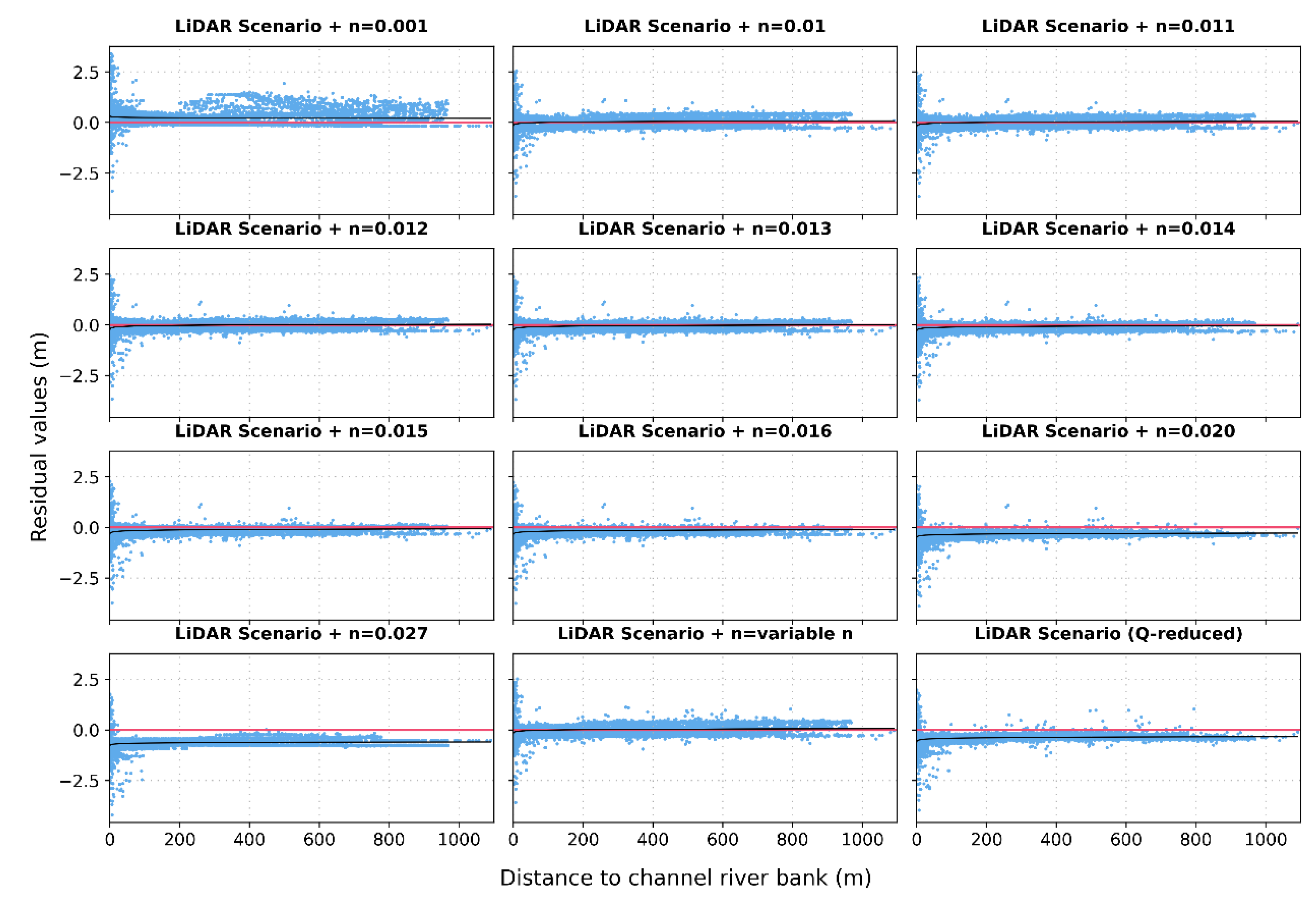
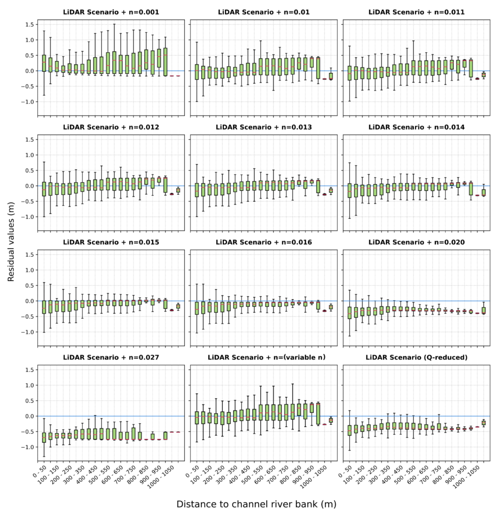
The results of the calibration of the Manning’s n value for the 500-year return period peak flow showed that the best fit varied according to the distance from the riverbank such that we could select different values of n (within a range between 0.011 and 0.014) depending on whether the area of greatest interest (in the hazard assessment) was close to the channel (lower value of n) or far from it (higher value of n). In any case, this implied the use of values of approximately half those used in real conditions. In the case of the 100-year return period peak flow, the best option of Manning’s value for areas far from the riverbank went up to 0.016.

-

A uniform Manning’s n value (for the river channel) was used both for the control “real scenario” and for each Manning’s n value calibrated model. However, a spatially distributed Manning’s n value was used too, and the results, although good, did not significantly improve on those obtained in the constant value models. In fact, it was observed that this model offered better results for distances up to 550 m from the riverbed, but at greater distances, the results worsen.

-

A hydraulic approach, namely, the HDCM, was also used, but the results were far from satisfactory. In fact, the results associated with this model were among the worst of those obtained in the present study. This situation calls into question the usefulness of this approach as a solution to the absence of bathymetric data in cases where the flow rates (on the date of acquisition of the topographic data, and those associated with the study) are very different.

-

The present work is the first contribution to a methodological framework that should be improved by applying it in other areas where the river characteristics (river slope, channel typology, sinuosity, percentage of reduction of the channel cross-section, etc.) are different from those shown in the present work. In this way, the objective of having a range of Manning’s n values depending on the specific characteristics of the study area could be achieved. This approach could represent an interesting scientific-technical innovation in the analysis of flood risks. Furthermore, in the present state, the use of “not natural lower Manning’s n value” was shown to be an optimal option for the improvement of flood damage estimates in urban areas where there is no availability of bathymetric data.

References

1. Istituto Centrale per il Restauro, Carta del Rischio, versione 2.1.1, Direzione Generale Sicurezza del Patrimonio Culturale (MIBACT). Available online: http://www.cartadelrischio.beniculturali.it/webgis/ (accessed on 30 October 2020).
2. Consiglio Nazionale Delle Ricerche, NOAH’s Ark project, CORDIS EU research results. Available online: https://cordis.europa.eu/project/id/501837 (accessed on 30 October 2020).
3. Lanza, S.G. Flood hazard threat on cultural heritage in the town of Genoa (Italy). J. Cult. Herit. 2003, 4, 159–167. [Google Scholar] [CrossRef]
4. Mazzanti, M. Valuing cultural heritage in a multi-attribute framework microeconomic perspectives and policy implications. J. Socio-Econ. 2003, 32, 549–569. [Google Scholar] [CrossRef]
5. Ortiz, R.; Ortiz, P.; Martín, J.M.; Vázquez, M.A. A new approach to the assessment of flooding and dampness hazards in cultural heritage, applied to the historic centre of Seville (Spain). Sci. Total Environ. 2016, 551–552, 546–555. [Google Scholar] [CrossRef]
6. Arrighi, C.; Brugioni, M.; Castelli, F.; Franceschini, S.; Mazzanti, B. Flood risk assessment in art cities: The exemplary case of Florence (Italy). J. Flood Risk Manag. 2018, 11, S616–S631. [Google Scholar] [CrossRef]
7. Figueiredo, R.; Romão, X.; Paupério, E. Flood risk assessment of cultural heritage at large spatial scales: Framework and application to mainland Portugal. J. Cult. Herit. 2020, 43, 163–174. [Google Scholar] [CrossRef]
8. CRED. The International Disaster Database [online], Centre for Research on the Epidemiology of Disasters. Available online: http://emdat.be/emdat_db/ (accessed on 10 April 2021).
9. Munich RE. NatCatSERVICE Database. Available online: https://natcatservice.munichre.com/ (accessed on 17 July 2020).
10. Ward, P.J.; Jongman, B.; Sperna Weiland, F.C.; Bouwman, A.; Van Beek, R.; Bierkens, M.; Ligtvoet, W.; Winsemius, H.C. Assessing flood risk at the global scale: Model setup, results, and sensitivity. Environ. Res. Lett. 2013, 8, 044019. [Google Scholar] [CrossRef]
11. Visser, H.; Bouwman, A.; Petersen, A.; Ligtvoet, W. A Statistical Study of Weather–Related Disasters: Past, Present and Future; PBL Netherlands Environmental Assessment Agency: The Hague, The Netherlands, 2012.
12. Merz, B.; Kreibich, H.; Schwarze, R.; Thieken, A. Assessment of economic flood damage. Nat Hazards Earth Syst. Sci. 2010, 10, 1697–1724. [Google Scholar] [CrossRef]
13. USACE. Economic Guidance Memorandum (EGM) 04-01, Generic Depth-Damage Relationships for Residential Structures with Basements; USACE: Washington, DC, USA, 2003. [Google Scholar]
14. Garrote, J.; Alvarenga, F.M.; Díez-Herrero, A. Quantification of flash flood economic risk using ultra-detailed stage–damage functions and 2-D hydraulic models. J. Hydrol. 2016, 541, 611–625. [Google Scholar] [CrossRef]
15. Huizinga, J.; De Moel, H.; Szewczyk, W. Global Flood Depth–Damage Functions: Methodology and the Database with Guidelines; Joint Research Centre: Luxembourg, 2017. [Google Scholar]
16. Deniz, D.; Arneson, E.E.; Liel, A.B.; Dashti, S.; Javernick-Will, A.N. Flood loss models for residential buildings, based on the 2013 Colorado floods. Nat. Hazards 2017, 85, 977–1003. [Google Scholar] [CrossRef]
17. Zabret, K.; Hozjan, U.; Kryžanowsky, A.; Brilly, M.; Vidmar, A. Development of model for the estimation of direct flood damage including the movable property. J. Flood Risk Manag. 2018, 11, S527–S540. [Google Scholar] [CrossRef]
18. Schoppa, L.; Sieg, T.; Vogel, K.; Zöller, G.; Kreibich, H. Probabilistic flood loss models for companies. Water Resour. Res. 2020, 56, e2020WR027649. [Google Scholar] [CrossRef]
19. Paprotny, D.; Kreibich, H.; Morales-Nápoles, O.; Castellarin, A.; Carisi, F.; Schröter, K. Exposure and vulnerability estimation for modelling flood losses to commercial assets in Europe. Sci. Total Environ. 2020, 737, 140011. [Google Scholar] [CrossRef]
20. Díez-Herrero, A.; Lain-Huerta, L.; Llorente-Isidro, M. A Handbook on Flood Hazard Mapping Methodologies; Publications of the Geological Survey of Spain (IGME): Madrid, Spain, 2009. [Google Scholar]
21. Casas, A.; Benito, G.; Thorndycraft, V.R.; Rico, M. The topographic data source of digital terrain models as a key element in the accuracy of hydraulic flood modelling. Earth Surf. Proc. Land. 2006, 31, 444–456. [Google Scholar] [CrossRef]
22. Bermúdez, M.; Zischg, A.P. Sensitivity of flood loss estimates to building representation and flow depth attribution methods in micro–scale flood modelling. Nat. Hazards 2018, 92, 1633. [Google Scholar] [CrossRef] [Green Version]
23. Dey, S.; Saksena, S.; Merwade, V. Assessing the effect of different bathymetric models on hydraulic simulation of rivers in data sparse regions. J. Hydrol. 2019, 575, 838–851. [Google Scholar] [CrossRef]
24. Arrighi, C.; Campo, L. Effects of digital terrain model uncertainties on high resolution urban flood damage assessment. J. Flood Risk Manag. 2019, 12, e12530. [Google Scholar] [CrossRef] [Green Version]
25. Vieux, B.E. Hydraulic Roughness. In Distributed Hydrologic Modeling Using GIS; Vieux, B.E., Ed.; Springer: Heidelberg, Germany, 2016; pp. 101–114. [Google Scholar] [CrossRef]
26. Boyer, M. Estimating the Manning coefficient from an average bed roughness in open channels. Eos. Trans. Am. Geophys. Union 1954, 35, 957–961. [Google Scholar] [CrossRef]
27. Kidson, R.; Richards, K.; Carling, P. Hydraulic model calibration for extreme floods in bedrock-confined channels: Case study from northern Thailand. Hydrol. Process. 2006, 20, 329–344. [Google Scholar] [CrossRef]
28. Ballesteros, J.; Bodoque, J.; Díez-Herrero, A.; Sanchez-Silva, M.; Stoffel, M. Calibration of floodplain roughness and estimation of flood discharge based on treering evidence and hydraulic modelling. J. Hydrol. 2011, 403, 103–115. [Google Scholar] [CrossRef]
29. Cook, A.; Merwade, V. Effect of topographic data, geometric configuration and modeling approach on flood inundation mapping. J. Hydrol. 2009, 377, 131–142. [Google Scholar] [CrossRef]
30. Boettle, M.; Kropp, J.P.; Reiber, L.; Roithmeier, O.; Rybski, D.; Walther, C. About the influence of elevation model quality and small-scale damage functions on flood damage estimation. Nat. Hazards Earth Syst. Sci. 2011, 11, 3327–3334. [Google Scholar] [CrossRef]
31. Kinzel, P.J.; Legleiter, C.J.; Nelson, J.M. Mapping River Bathymetry with a Small Footprint Green LiDAR: Applications and Challenges. J. Am. Water Resour. Ass. (JAWRA) 2012, 49, 183–204. [Google Scholar] [CrossRef]
32. Allouis, T.; Bailly, J.S.; Pastol, Y.; LeRoux, C. Comparison of LiDAR Waveform Processing Methods for Very Shallow Water Bathymetry Using Raman, Near-Infrared and Green Signals. Earth Surf. Proc. Land. 2010, 35, 640–650. [Google Scholar] [CrossRef]
33. Bangen, S.G.; Wheaton, J.M.; Bouwes, N.; Bouwes, B.; Jordan, C. A methodological intercomparison of topographic survey techniques for characterizing wadeable streams and rivers. Geomorphology 2014, 206, 343–361. [Google Scholar] [CrossRef]
34. Hostache, R.; Matgen, P.; Giustarini, L.; Teferle, F.N.; Tailliez, C.; Iffly, J.; Corato, G. A drifting GPS buoy for retrieving effective riverbed bathymetry. J. Hydrol. 2015, 520, 397–406. [Google Scholar] [CrossRef] [Green Version]
35. Fonstad, M.A.; Marcus, W.A. Remote sensing of stream depths with hydraulically assisted bathymetry (HAB) models. Geomorphology 2005, 72, 320–339. [Google Scholar] [CrossRef]
36. Trigg, M.A.; Wilson, M.D.; Bates, P.D.; Horritt, M.S.; Alsdorf, D.E.; Forsberg, B.R.; Vega, M.C. Amazon flood wave hydraulics. J. Hydrol. 2009, 374, 92–105. [Google Scholar] [CrossRef]
37. Gichamo, T.Z.; Popescu, I.; Jonoski, A.; Solomatine, D. River cross-section extraction from the ASTER global DEM for flood modeling. Environ. Model. Softw. 2012, 31, 37–46. [Google Scholar] [CrossRef]
38. Grimaldi, S.; Li, Y.; Walker, J.P.; Pauwels, V.R.N. Effective representation of river geometry in hydraulic flood forecast models. Water Resour. Res. 2018, 54, 1031–1057. [Google Scholar] [CrossRef]
39. Bradbrook, K.F.; Lane, S.N.; Waller, S.G.; Bates, P.D. Two dimensional diffusion wave modelling of flood inundation using a simplified channel representation. Int. J. River Basin Manag. 2004, 2, 211–223. [Google Scholar] [CrossRef]
40. Choné, G.; Biron, P.M.; Buffin-Bélanger, T. Flood hazard mapping techniques with LiDAR in the absence of river bathymetry data. In E3S Web of Conferences, Proceedings of the River Flow 2018—Ninth International Conference on Fluvial Hydraulics, Lyon, France, 5–8 September 2018; EDP Science: Les Ulis, France, 2018; Abstract 06005. [Google Scholar]
41. Wolman, M.G.; Miller, J.P. Magnitude and Frequency of Forces in Geomorphic Processes. J. Geol. 1960, 68, 54–74. [Google Scholar] [CrossRef] [Green Version]
42. Ardıçlıoğlu, M.; Kuriqi, A. Calibration of channel roughness in intermittent rivers using HEC-RAS model: Case of Sarimsakli creek, Turkey. SN Appl. Sci. 2019, 1, 1080. [Google Scholar] [CrossRef] [Green Version]
43. Hawker, L.; Bates, P.; Neal, J.; Rougier, J. Perspectives on Digital Elevation Model (DEM) Simulation for Flood Modeling in the Absence of a High-Accuracy Open Access Global DEM. Front. Earth Sci. 2018, 6, 233. [Google Scholar] [CrossRef] [Green Version]
44. Instituto Geográfico Nacional, LiDAR PNOA. 2014. Available online: https://pnoa.ign.es/el-proyecto-pnoa-lidar (accessed on 30 October 2020).
45. Arcement, G.J.; Schneider, V.R. Guide for Selecting Manning’s Roughness Coefficients for Natural Channels and Flood Plains; USGS: Denver, CO, USA, 1989.
46. Brunner, G.W. HEC-RAS, River Analysis System Hydraulic Reference Manual, Version 4.1; U.S. Army Corps of Engineers: Davis, CA, USA, 2010. [Google Scholar]
47. Bladé, E.; Cea, L.; Corestein, G.; Escolano, E.; Puertas, J.; Vázquez-Cendón, E.; Dolz, J.; Coll, A. Iber: Herramienta de simulación numérica del flujo en ríos. Rev. Intern. Met. Num. Calc. Dis. Ingen. 2014, 30, 1–10. [Google Scholar] [CrossRef] [Green Version]
48. ESRI. ArcMap. 2011. Available online: https://desktop.arcgis.com/es/arcmap/ (accessed on 30 October 2020).
49. Hunter, J.D. Matplotlib: A 2D Graphics Environment. Comput. Sci. Eng. 2007, 9, 90–95. [Google Scholar] [CrossRef]
50. Bates, P.D.; De Roo, A.P.J. A simple raster-based model for flood inundation simulation. J. Hydrol. 2000, 236, 54–77. [Google Scholar] [CrossRef]
51. Horritt, M.S.; Bates, P.D. Evaluation of 1D and 2D numerical models for predicting river flood inundation. J. Hydrol. 2002, 268, 87–99. [Google Scholar] [CrossRef]
52. Tayefi, V.; Lane, S.N.; Hardy, R.J.; Yu, D. A comparison of one- and two dimensional approaches to modelling flood inundation over complex upland floodplains. Hydrol. Process. 2007, 21, 3190–3202. [Google Scholar] [CrossRef]
53. Saleh, F.; Ducharne, A.; Flipo, N.; Oudin, L.; Ledoux, E. Impact of river bed morphology on discharge and water levels simulated by a 1D Saint—Venant hydraulic model at regional scale. J. Hydrol. 2012, 476, 1–9. [Google Scholar] [CrossRef]
54. Casas, A.; Lane, S.; Hardy, R.J.; Benito, G.; Whiting, P.J. Reconstruction of subgrid-scale topographic variability and its effect upon the spatial structure of three-dimensional river flow. Water Resour. Res. 2010, 46, W03519. [Google Scholar] [CrossRef] [Green Version]
55. Casas, A.; Stuart, L.; Dapeng, Y.; Benito, G. A method for parameterising roughness and topographic sub-grid scale effects in hydraulic modelling from LiDAR data. Hydrol. Earth Syst. Sci. 2010, 14, 1567–1579. [Google Scholar] [CrossRef] [Green Version]
56. Benito, G.; Díez-Herrero, A. Palaeoflood Hydrology: Reconstructing Rare Events and Extreme Flood Discharges. In Hydro-Meteorological Hazards, Risks, and Disasters; Paron, P., Di Baldassarre, G., Eds.; Elsevier: Amsterdam, The Netherlands, 2015; pp. 65–104. [Google Scholar]
57. Cowan, W.L. Estimating hydraulic roughness coefficients. Agr. Eng. 1956, 37, 473–475. [Google Scholar]
58. Chow, V.T. Open-Channel Hydraulics; McGraw-Hill Book Co.: New York, NY, USA, 1959; 680p. [Google Scholar]
59. Ercan, A.; Kavvas, M.L. Scaling and self-similarity in two-dimensional hydrodynamics. Chaos 2015, 25, 075404. [Google Scholar] [CrossRef] [PubMed]
60. Larsen, L.G.; Ma, J.; Kaplan, D. How Important Is Connectivity for Surface Water Fluxes? A Generalized Expression for Flow Through Heterogeneous Landscapes. Geophys. Res. Lett. 2017, 44, 10349–10358. [Google Scholar] [CrossRef]
61. Prior, E.M.; Aquilina, C.A.; Czuba, J.A.; Pingel, T.J.; Hession, W.C. Estimating Floodplain Vegetative Roughness Using Drone-Based Laser Scanning and Structure from Motion Photogrammetry. Remote Sens. 2021, 13, 2616. [Google Scholar] [CrossRef]
62. Limerinos, J.T. Determination of the Manning Coefficient from Measured Bed Roughness in Natural Channels; United States Geological Survey: Washington, DC, USA, 1970; 53p.
63. Simons, D.B.; Richardson, E.V. Resistance to Flow in Alluvial Channels; United States Geological Survey: Washington, DC, USA, 1966; 70p.
64. Horritt, M.S. A linearized approach to flow resistance uncertainty in a 2-D finite volume model of flood flow. J. Hydrol. 2006, 316, 13–27. [Google Scholar] [CrossRef]
65. Timbadiya, P.V.; Patel, P.L.; Porey, P.D. Calibration of HEC-RAS model on prediction of flood for lower Tapi River, India. J. Water Resour. Prot. 2011, 3, 805–811. [Google Scholar] [CrossRef] [Green Version]
66. Attari, M.; Hosseini, S.M. A simple innovative method for calibration of Manning’s roughness coefficient in rivers using a similarity concept. J. Hydrol. 2019, 575, 810–823. [Google Scholar] [CrossRef]
67. Wagenaar, D.J.; de Bruijn, K.M.; Bouwer, L.M.; de Moel, H. Uncertainty in flood damage estimates and its potential effect on investment decisions. Nat. Hazards Earth Syst. Sci. 2016, 16, 1–14. [Google Scholar] [CrossRef] [Green Version]
68. FEMA. Federal Emergency Management Agency, Flood Map, Flood Insurance Rate Map (FIRM). 2009. Available online: https://floodpartners.com/fema-flood-map/ (accessed on 30 October 2020).
69. Dirección General del Agua, Sistema Nacional de Cartografía de Zonas Inundables (SNCZI). 2013. Available online: https://sig.mapama.gob.es/snczi/index.html?herramienta=DPHZI (accessed on 25 October 2020).
70. First Street Foundation, Flood Factor. 2019. Available online: https://floodfactor.com/ (accessed on 27 October 2020).
Figure 1. The study area and cultural heritage sites location map (A). The digital elevation model (DEM) from LiDAR data (B) not showing bathymetry, which was included from echo sounders with a D-GPS (C). Example of a cross-section flow depth calibration (D).
Applsci 11 09267 g001
Figure 2. Flow chart of the full methodological approach that was used in the Manning’s n value calibration process, from data sources until the calibrated vs. control scenarios comparison.
Applsci 11 09267 g002
Figure 3. Basic conceptual diagram for the calibration of the parameter n, assuming that the flow rate (Q) is a function of the cross-sectional area of the channel (A1 and A2) and the mean flow velocity (V1 and V2, which, in turn, is dependent on the Manning’s n values (n1 and n2)). The size of the symbols identifying the variables is directly related to the magnitude of the variables.
Applsci 11 09267 g003
Figure 4. Topographic differences between the “real scenario” and the “LiDAR scenario” (A), where green colors show lower differences and red colors show higher topographic differences. A grouping analysis (B) of the errors without spatial constraints showed a non-uniform pattern.
Applsci 11 09267 g004
Figure 5. Map showing the spatial distribution of the Manning’s n value best fit option along the Douro River channel in Zamora city, Spain. The Manning’s n value best fit was found from the relationship between the channel bathymetry differences (“real scenario”–“LiDAR scenario”) and the flow depth differences.
Applsci 11 09267 g005
Figure 6. Scatter plot graphical representation of the relationship between the variable flow depth and distance to the riverbank for different Manning’s n value calibrated models. The red line shows an error equal to zero and the black line shows a logarithmic fitting to the point values.
Applsci 11 09267 g006
Figure 7. Box plot graphics showing the relationship between the flow depth errors and the distance to the riverbank (within 50 m intervals). Positive errors were related to the underestimation of the flow depth value by the calibrated model, and vice versa.
Applsci 11 09267 g007
Figure 8. Local Manning’s n value calibration results at control points in Zamora city. The upper and lower graphs show flow depth values for each calibrated model, where the red line shows the flow depth value for the control model, i.e., the “real scenario”.
Applsci 11 09267 g008