Article

The Effect of the Wenchuan and Lushan Earthquakes on the Size Distribution of Earthquakes along the Longmenshan Fault

1
Key Laboratory of Environmental Change and Natural Disaster, Beijing Normal University, Beijing 100875, China
2
State Key Laboratory of Earth Surface Processes and Resource Ecology, Beijing Normal University, Beijing 100875, China
3
Center for Geodata and Analysis, Faculty of Geographical Science, Beijing Normal University, Beijing 100875, China
4
National Tibetan Plateau Data Center, Beijing 100101, China
5
College of Data Science, Taiyuan University of Technology, Taiyuan 030024, China
*
Author to whom correspondence should be addressed.
Appl. Sci. 2021, 11(18), 8534; https://doi.org/10.3390/app11188534
Submission received: 10 August 2021 / Revised: 9 September 2021 / Accepted: 11 September 2021 / Published: 14 September 2021
(This article belongs to the Special Issue Geohazards: Risk Assessment, Mitigation and Prevention)

Abstract

:
Changes in the stress state of faults and their surroundings is a highly plausible mechanism explaining earthquake interaction. These stress changes can impact the seismicity rate and the size distribution of earthquakes. However, the effect of large earthquakes on the earthquake size distribution along the Longmenshan fault has not been quantified. We evaluated the levels of the b value for the stable state before and after the large earthquakes on 12 May 2008 (Wenchuan, MS 8.0) and 20 April 2013 (Lushan, MS 7.0) along the Longmenshan fault. We found that after the mainshocks, the size distribution of the subsequent earthquakes shifted toward relatively larger events in the Wenchuan aftershock zone (b value decreased from 1.21 to 0.84), and generally remained invariable in the Lushan aftershock zone (b value remained at 0.76). The time required for the b value to return to stable states after both mainshocks was entirely consistent with the time needed by the aftershock depth images to stop visibly changing. The result of the temporal variation of b values shows decreasing trends for the b value before both large earthquakes. Our results are available for assessing the potential seismic risk of the Longmenshan fault as a reference.

1. Introduction

Following the Wenchuan MS 8.0 earthquake on 12 May 2008, the Longmenshan fault zone was struck by the 20 April 2013 MS 7.0 Lushan earthquake. The Longmenshan fault zone is composed of several almost parallel thrust faults, forming a boundary fault between the Sichuan Basin and Tibetan Plateau, and controls the seismicity of the Longmenshan region (Figure 1). The epicenters of the Wenchuan and Lushan earthquakes were approximately 87 km apart, and the focal mechanism of both events showed a thrust rupture [1].
According to the characteristics of the Wenchuan and Lushan earthquakes, whether the MS 7.0 Lushan event was a strong aftershock of the MS 8.0 Wenchuan earthquake or a new and independent event has been a topic of debate. For example, some researchers suggest that the two large earthquakes were independent events. The reasons are as follows: (1) there is no overlapping area between the Wenchuan and Lushan earthquake rupture zones [2]; (2) the Wenchuan and Lushan earthquakes were generated in different faults in the Longmenshan fault zone [3]; (3) the rupture processes of the Wenchuan and Lushan earthquakes were different, and the aftershock zones of the two events were nearly 45 km apart [4]. Alternatively, some scientists propose that the Wenchuan and Lushan earthquakes were a mainshock–aftershock sequence and note that the Lushan event struck in an area where Coulomb stress was increased due to the Wenchuan earthquake [5,6].
The controversy over the relationship between the Wenchuan and Lushan earthquakes highlights the complexity of earthquake interaction in the Longmenshan fault zone. It is widely accepted that earthquake interactions can be understood by identifying changes in static and dynamic stress states around faults [7,8,9]. The most observable effect of this stress change is a significant increase in seismicity rate, which is generally considered an aftershock phenomenon [10,11,12]. Statistically, aftershock activity is classically described by n(t) = K/(t + c)p, where n(t) is the number of aftershocks after time t and K, c, and p are constants that describe the aftershock productivity [13]. Ogata [14,15] described aftershock activity as a multigenerational branching process and proposed the epidemic-type aftershock sequence model, which is a stochastic point process model of self-exciting point processes.
Changes in stress can impact the seismicity rate and the frequency size distribution, which is alternatively known as the frequency-magnitude distribution (FMD) [16] or Gutenberg–Richter (G–R) law [17] and is expressed as logN = ab M, where N is the number of events in a given time period with magnitude greater than M, a describes the seismicity of a given seismogenic volume, and b is the slope of the FMD. Previous studies showed that b values fall within the range of 1.02 ± 0.03 on a large scale for a long time [18,19]. For regions on a smaller scale, the b values show a broad range of spatial and temporal variations. For example, the b value ranged from 0.5 to 2.5 in the Andaman–Sumatra region and California [20]. Interpretation of the variation of b values is based on several factors, including stress state [21,22], focal depth [23], faulting style [24,25], fluid pressure [26], and so on.
The earthquake size distribution generally follows a power law, with a slope of b values, which characterizes the relative occurrence of large and small events. A low b value indicates a larger proportion of large earthquakes and vice versa. Zhao et al. [27] (2008) compared the spatial footprint of b values before and after the Wenchuan earthquake in the Longmenshan fault zone, and the results showed that the b values tend to change from lower in the southern region to higher in the northeastern region. The temporal change in b values before the Wenchuan MS 8.0 earthquake showed a decreasing trend [28,29,30], and the Lushan MS 7.0 earthquake showed similar temporal change trends in b values [31]. These studies focused on the variation trend of b values before and after the two large events along the Longmenshan fault. However, the fundamental effect of the Wenchuan and Lushan earthquakes on the size distribution of earthquakes along the Longmenshan fault has not been quantified, which limits our understanding of how the apparent stress changes in the region affect the size distribution of earthquakes.
In this study, we evaluated the spatiotemporal evolution of the b values along the Longmenshan fault in the past nearly 20 years. Moreover, we estimated the levels of the b value for the stable state before and after the Wenchuan and Lushan earthquakes and quantified the effects of the two large earthquakes on the size distribution of subsequent events at different times. In addition, the spatial evolution process of the deep seismogenic environment in the Wenchuan and Lushan aftershock zones in two and three dimensions was illustrated via spatial scanning and data fitting, which can be used to analyze the aftershock activity of the two large earthquakes.

2. Data and Postulates

The earthquake catalog we used here was documented by the regional seismic network and then verified by the China Earthquake Networks Center (CENC) along the Longmenshan fault during the period from 1 January 2000 to 1 January 2019. It is a relatively complete catalog containing the Wenchuan-Lushan earthquake sequence.
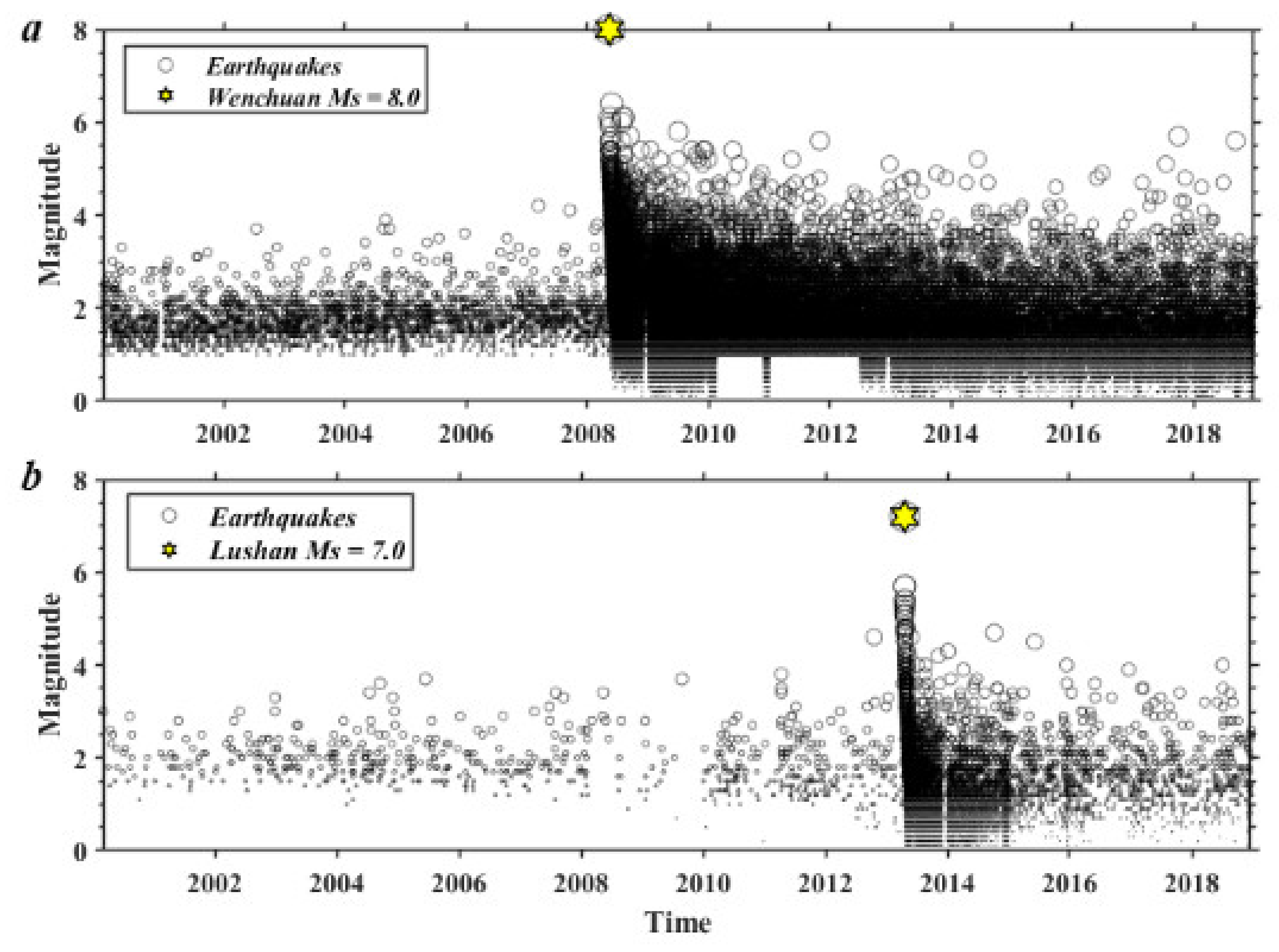
Figure 2 shows the magnitude-time distribution of earthquakes in the Wenchuan source region and Lushan source region. The locations of the earthquakes in this catalog were corrected for accuracy. Each event includes the time, location, magnitude, and depth. Homogeneity of the catalog was iterated and optimized for subsequent research and analysis.
Stress change has been widely used to interpret the triggering of the mainshock–mainshock and mainshock–aftershock events [7,32,33,34,35,36]. However, the exact measurement of stress states is difficult; thus, a relationship between the stress state and b value has been proposed [16,24,37,38]. Schorlemmer et al. [24] demonstrated that the b value could be regarded as a stress indicator that depends inversely on differential stress. Therefore, changes in the stress state on faults lead to the variation in b values, which is followed by time-dependent recovery. In general, the larger the magnitude of the earthquake, the greater the stress changes and the larger the b value fluctuations. No event of magnitude larger than MS 7.0 had been reported in the historical record of the Longmenshan fault zone and the catalog we used in this paper contains more than 80,000 events and only two large earthquakes greater than magnitude 6.5, that is, the Wenchuan MS 8.0 and Lushan MS 7.0 earthquakes. Thus, these two events are mainly responsible for the apparent changes in stress state along the Longmenshan fault zone in the past 20 years.
Therefore, there are two postulates: first, without a large earthquake perturbation, the b value will remain in a stable state with a small fluctuation range for a long time; second, after the perturbation of a large earthquake, the b value may recover to another stable state. We evaluated the levels of the b value for the stable state before and after these two large earthquakes in the study region.

3. Methods

The main methods we used include estimation methods (MaxCurvature for the estimation of the completeness magnitude; maximum likelihood estimation (MLE) for the b value estimation), test methods (Akaike information criterion (AIC) for the variation trend of b values; the nonlinearity index (NLIndex) for the linearity assessment of frequency-magnitude distribution) and kriging interpolation to describe the spatial and temporal evolution images of aftershock focal depth.

3.1. Completeness Magnitude (MC) and b Value Estimation

The estimation of the completeness of earthquake catalogs is essential to the computation of b values, and the lowest magnitude of all earthquakes that are reliably detected in a space-time volume is defined as the completeness magnitude (MC) [39]. The lower the MC, the higher the detection capability. Here, we use the MaxCurvature technique, which estimates the MC by locating the magnitude that is the highest frequency of events in the FMD. Mignan [40] showed that the MaxCurvature technique underestimates the MC in cases involving gradually curved FMDs and postulated that this underestimation tendency arises from spatiotemporal heterogeneities within the earthquake monitoring network. Therefore, we used the corrected MaxCurvature method with a correction factor of +0.2 [41], and the uncertainties were determined by bootstrapping.
The least-squares method and maximum likelihood estimation are often used to calculate the b value, and the latter approach is considered more stable. In this work, the maximum likelihood estimation used to calculate the b value and its standard deviation [42,43]:
b = 1 ln ( 10 ) ( M ¯ M C )
where M ¯ is the average magnitude of earthquakes with M ≥ MC; MC is the cutoff magnitude. The confidence limit of the b value is expressed as follows:
σ = b N
where N is the number of earthquake cases of the given sample.

3.2. Estimation of the Frequency-Magnitude Distribution (FMD) Extrapolation

The nonlinearity index (NLIndex) can be used to assess whether the extrapolation of a given high-magnitude FMD is likely an overestimate or underestimate of the probable rates for large events [44].
(1)
Calculate the b value for all Mcut from Mcmin to the highest Mcut for which Nmin events are still sampled.
(2)
Divide the standard deviation by the largest individual b value uncertainty for each possible Mcut, and for each Mcut, this value is the NLIndex.
(3)
Divide the NLIndex for each Mcut by the number of estimated b values to weight the result by data density. Please check Italics.
(4)
Find the minimum weighted NLIndex to find the best MC that produces the most linear FMD fit.
If NLIndex ≤ 1, the FMD is regarded as linear, and if NLIndex > 1, the FMD is not linear. The slope of Mcut is clearly positive or negative, respectively, indicating that the FMD overestimates or underestimates large M rates.

3.3. Akaike Information Criterion

To quantify the changing trend of b values, the P test was conducted for b values in two sample windows based on the Akaike information criterion (AIC) [45]. Hypothesis 1: the b values in the two sample windows are the same; Hypothesis 2: the b values in the two sample windows are different, represented as b1 and b2, respectively. The hypothesis of the difference of the AIC leads to the difference ΔAIC [46]:
Δ A I C = 2 ( N 1 + N 2 ) ln ( N 1 + N 2 ) + 2 N 1 ln ( N 1 + N 2 b 1 b 2 ) + 2 N 2 ln ( N 2 + N 1 b 2 b 1 ) 2
where Ni is the number of events in the sample windows and bi is b values in the sample windows. Pb represents the probability that the events in the two sample windows come from the same population and can be derived from the AIC as follows:
P b = e ( Δ A I C / 2 ) 2
The b value in the sample window represents a significant change when ΔAIC ≥ 2 (Pb ≈ 0.05) and is highly significant when ΔAIC > 5 (Pb ≈ 0.01) [47].

3.4. Kriging Interpolation

Kriging interpolation is the most commonly used geostatistical approach for spatial interpolation. With this method, a semivariogram is used to express the spatial relationship of the distance between samples. This technique depends on the spatial model between samples to predict attribute values at unsampled locations [48]. As a widely used interpolation method, kriging takes into account the distance between unknown positions and the sample locations as well as the distance between sample locations, effectively reducing the interference of clustering in samples on the accuracy of the interpolated estimates [49]. We used the kriging interpolation algorithm to produce maps incorporating anisotropy and underlying trends from irregularly spaced data. The exponential semivariance model with the smallest prediction errors was chosen over the Gaussian and spherical models for the spatial interpolation of focal depth data.

4. Results and Analysis

4.1. Completeness Magnitude (MC) and Linearity Assessment of Frequency-Magnitude Distribution (FMD)

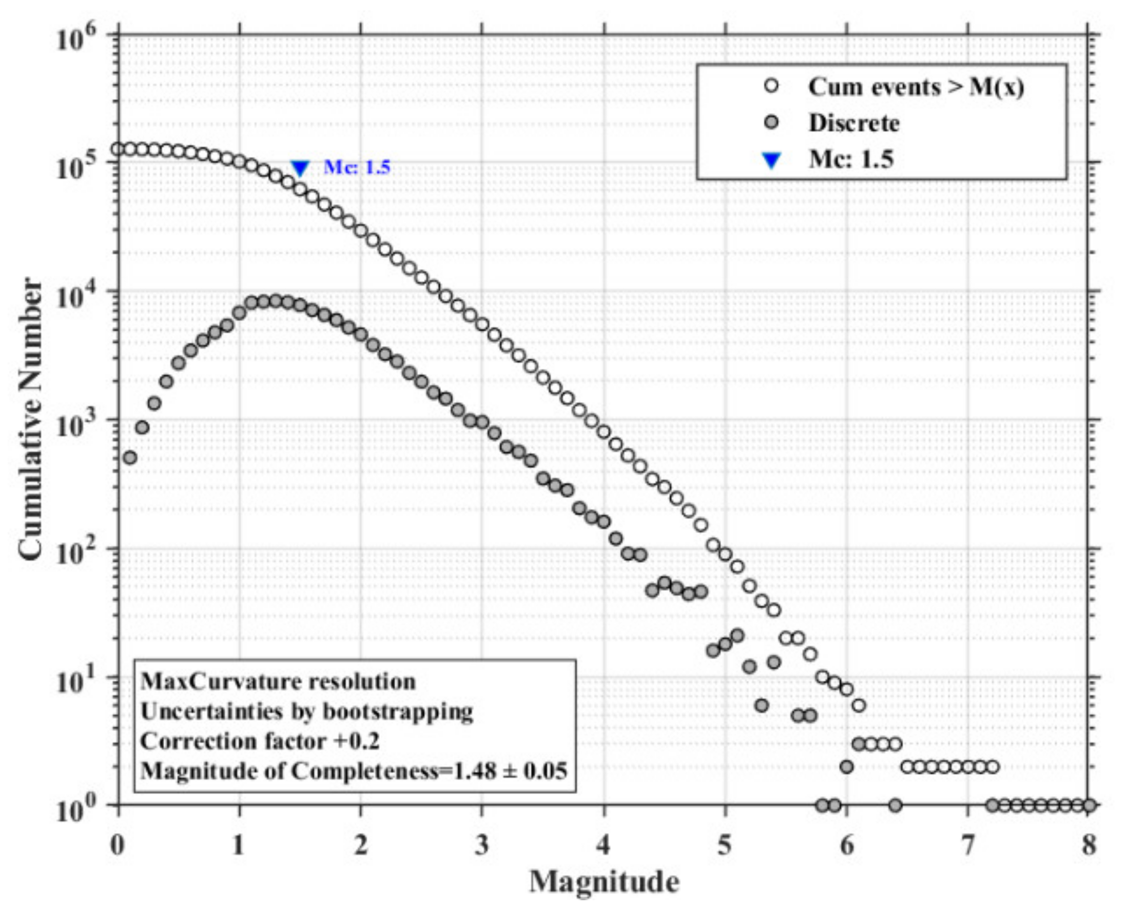
As shown in Figure 3, the results of the corrected MaxCurvature method show that the MC of the earthquake catalog used in this work is MC = 1.5. This result is consistent with the results of previous studies on the Wenchuan earthquake zone [30,50]. Fang et al. [51] described in detail the aftershock performance and analysis of the Lushan earthquake based on the combined data from permanent and temporary seismic stations. They concluded that the minimum complete magnitude was M = 1.0. To unify the consistency of the MC of the Wenchuan MS 8.0 and Lushan MS 7.0 earthquakes in the Longmenshan fault zone, we selected events with magnitudes of MMC = 1.5.
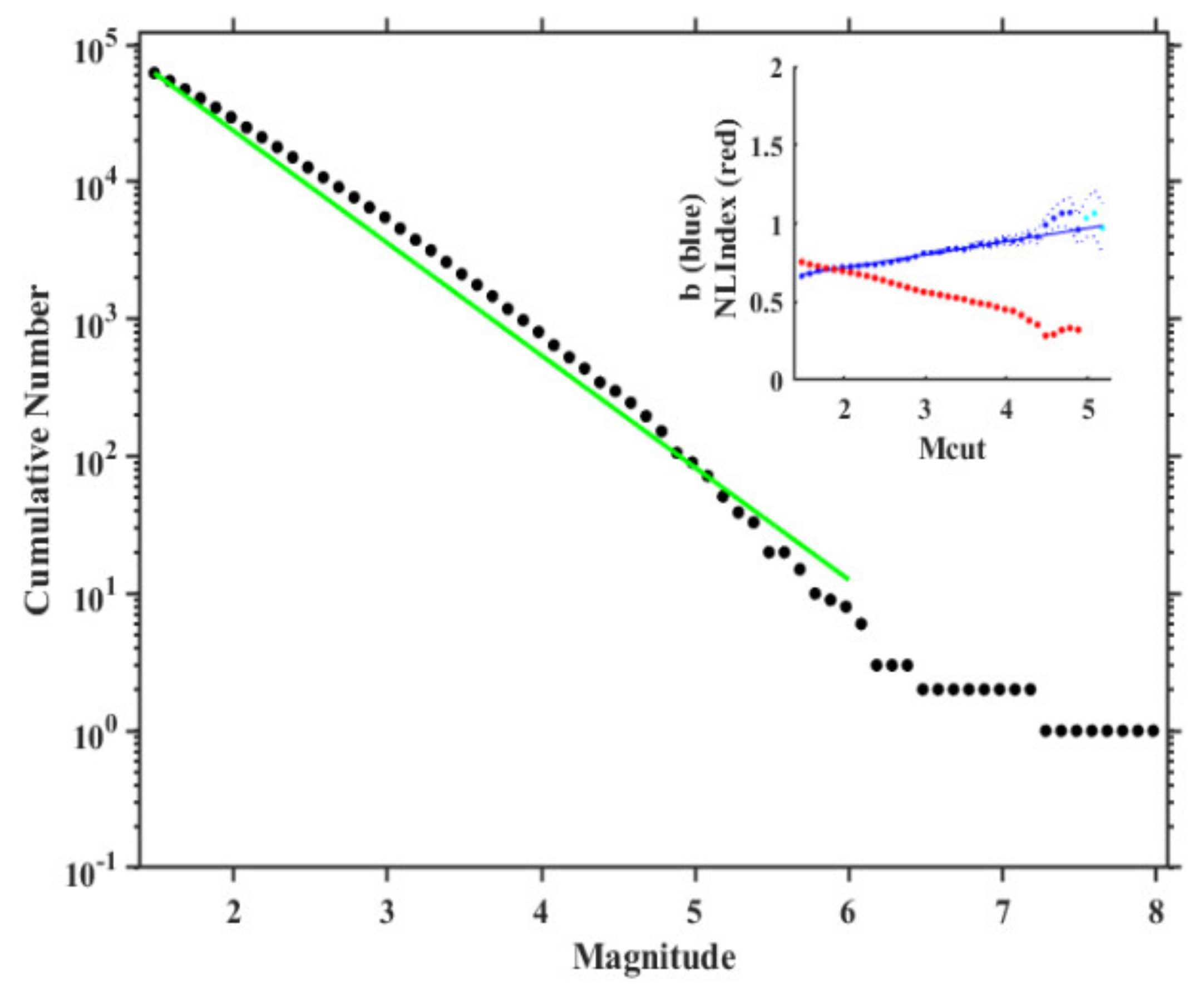
We performed a linearity check on FMD, and the results are shown in Figure 4. The NLIndex (red) is shown for different cutoff magnitudes (upper inset) and the NLIndex ≤ 1 for all cut off magnitudes; thus, the linear FMD is accepted as the best MC.

4.2. Time-Space Analysis of b Values

Earthquake frequency will increase immediately within a short time after a large event and may exceed the recording capacity of the seismic network. Before establishing the time-space series of b values with aftershocks, we should eliminate the events documented in the early catalog, which is somewhat heterogeneous and incomplete in small events [41]. In this work, the exclusion period depends on the magnitude of completeness over time. Therefore, we first removed the events documented in the initial catalog within two months after the Wenchuan MS 8.0 and Lushan MS 7.0 earthquakes, a period for which the data are highly incomplete. Then, we calculated the spatiotemporal distributions of b values before and after two large events that occurred from 2000–2019 along the Longmenshan fault by selecting events with MMC = 1.5 and using a time window and spatial grid to calculate the b values. In this computation, the window lengths were set to at least 500 events in the Wenchuan aftershock zone and 200 events in the Lushan aftershock zone. Each window was moved forward by one event at a time.
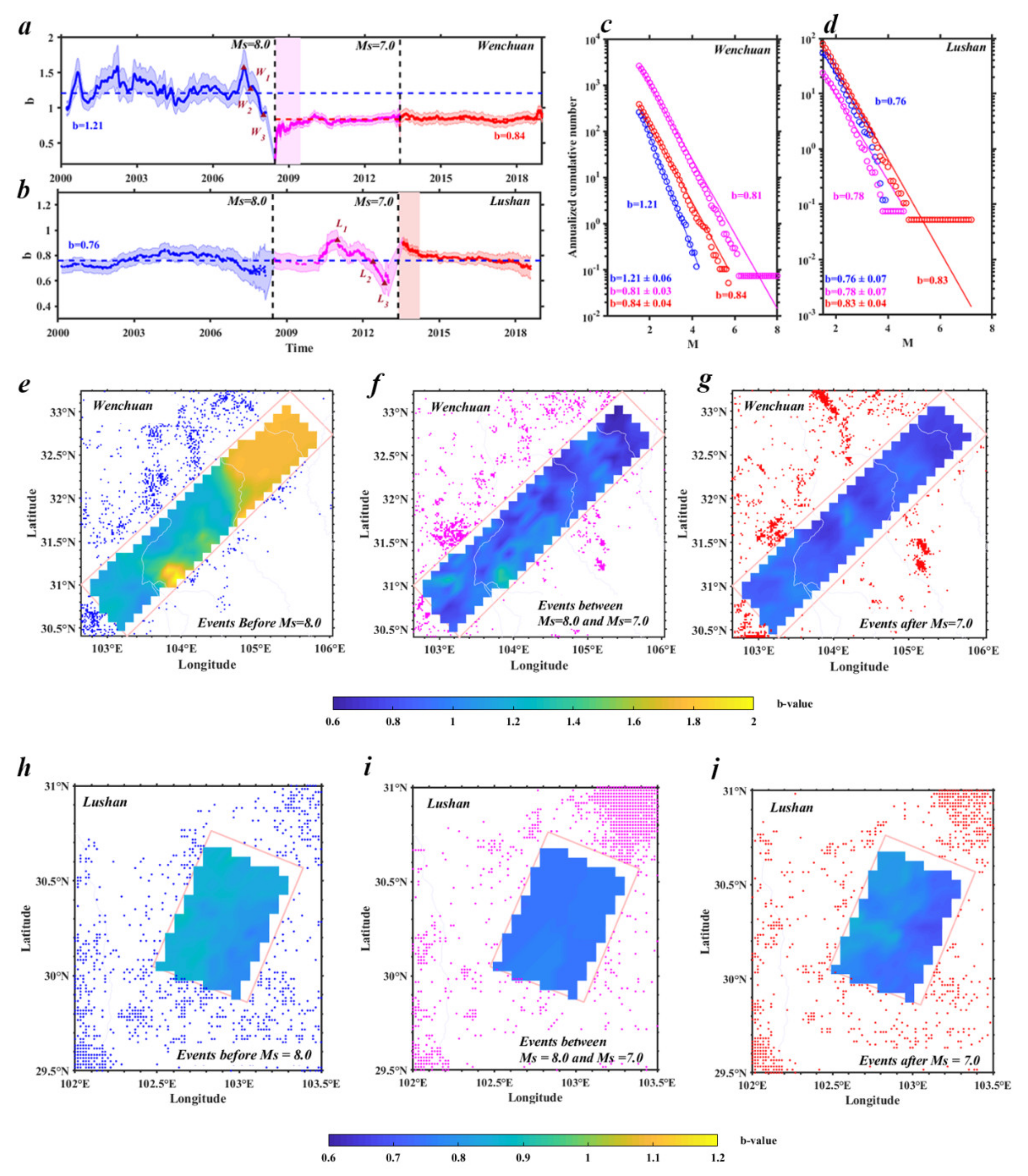
Figure 5a,b display time series of the b value in source regions, and the overall change trend conforms to our postulation that b values will undergo relatively significant changes in a period of time before and after a large earthquake. Specifically, b values show a decreasing trend before the occurrence of both large earthquakes in both zones. To ensure that this trend is statistically significant, we quantitatively assessed the temporal variation in b values using the P parameter test and selected three windows before the MS 8.0 event (W1, W2, and W3) and the MS 7.0 event (L1, L2, and L3). Window selection was based on the significance of changes in b values (Figure 5a,b). The results are shown in Table 1. The b value in the sample window has significantly changed when ΔAIC ≥ 2 (Pb ≈ 0.05). Table 1 shows that the b values decreased before both large earthquakes with statistically significant variations.
After the Wenchuan MS 8.0 event, the b values in the Wenchuan aftershock zone experienced a period of dramatic fluctuation (indicated by the pink shading lasting not more than one year) before gradually stabilizing within a small fluctuation range (Figure 5a), which was similar to the range of b values in the third period (Figure 5c, b = 0.84). After the Lushan MS 7.0 event, the b values in the Lushan aftershock zones increased rapidly and then slowly dropped to a stable state (Figure 5b), which was similar to the FMD in the first period (Figure 5d, b = 0.76). As shown in Figure 5b (red shading), the b value required less than ten months to return to a stable state.
The reference b values can be estimated for the background levels (for the period, b = 1.21 in the Wenchuan aftershock zone and b = 0.76 in the Lushan aftershock zone). When the perturbation effect of the mainshocks gradually decreases, the b values in the Lushan aftershock zone eventually return to the background level (b = 0.76), whereas those in the Wenchuan aftershock zone drop below the background level (from 1.21 to 0.84). To date, there have been no earthquakes that have significantly changed the stability of the Longmenshan fault zone since the MS 7.0 Lushan earthquake.
The temporal distribution of earthquakes also indicates the change in stress state of faults and their surroundings. As shown in Figure 2a, before the MS 8.0 Wenchuan earthquake, the frequency of events in the Wenchuan aftershock zone had been decreasing for a year since 2006, and only two events greater than MS 4 occurred during the period when b values were significantly decreasing (Figure 5a). However, earthquakes that were greater than MS 4 struck the entire Wenchuan aftershock zone after the MS 8.0 event (Figure 1). In addition, there were no strong aftershocks above magnitude 6.5 along the faults, and only six events greater than MS 4 occurred within two months after the mainshock. These phenomena indicate that without the continuous perturbation of strong aftershock, the b value gradually stabilized to the state mainly determined by the background earthquakes, which tended to shift to larger events following the MS 8.0 event in the Wenchuan aftershock zone.
After the MS 8.0 Wenchuan earthquake, the Lushan aftershock zone also experienced a “seismic quiescence” of approximately two years, and only one event greater than MS 4 occurred before the MS 7.0 Lushan earthquake during the period when b values were significantly decreasing (Figure 2b). Moreover, only a few events greater than MS 4 occurred within two months after the mainshock; the subsequent events basically returned to the magnitude of the background earthquakes before the mainshock, which shows that the b values in the Lushan aftershock zone eventually returned to the background level (Figure 5b).
To analyze the spatial footprints of the changes in the b values, we divided the two study regions into 0.1° × 0.1° grids, sampled the 300 events nearest to each grid node within radius of 30 km, and re-estimated the MC in each node. For this purpose, we used a bootstrap approach to sample the events 1000 times randomly. The spatial footprints of the changes in the b values are consistent with the FMDs (Figure 5c,d). Figure 5e–g demonstrate the spatial variation in the b values throughout the Wenchuan aftershock zone. Figure 5h–j show the spatial variation in the b values in the Lushan aftershock zone.
The b value in the southern part of the Wenchuan source region and Lushan source region was lower than that in the northern part of the Wenchuan aftershock before the MS 8.0 Wenchuan event (Figure 5e,h). This pattern is consistent with the characteristics of the Longmenshan fault, which is a strike-slip fault in the north and a thrust fault in the southern section. It is generally considered that the b value is inversely proportional to stress, and the b values of different types of faults are as follows: b (normal) > 1, b (strike-slip)~1, and b (thrust) < 1 [24,25]. The conditions changed markedly after the MS 8.0 Wenchuan event; the b values decreased in the Wenchuan source region and Lushan source region (Figure 5f,i). This finding illustrates the effect of the Wenchuan earthquakes on stress change along the Longmenshan fault. Figure 5g,j illustrate the stable state of the b value in the Longmenshan fault zone.

4.3. Evolution of Images of Aftershock Activity Depicted by Focal Depth

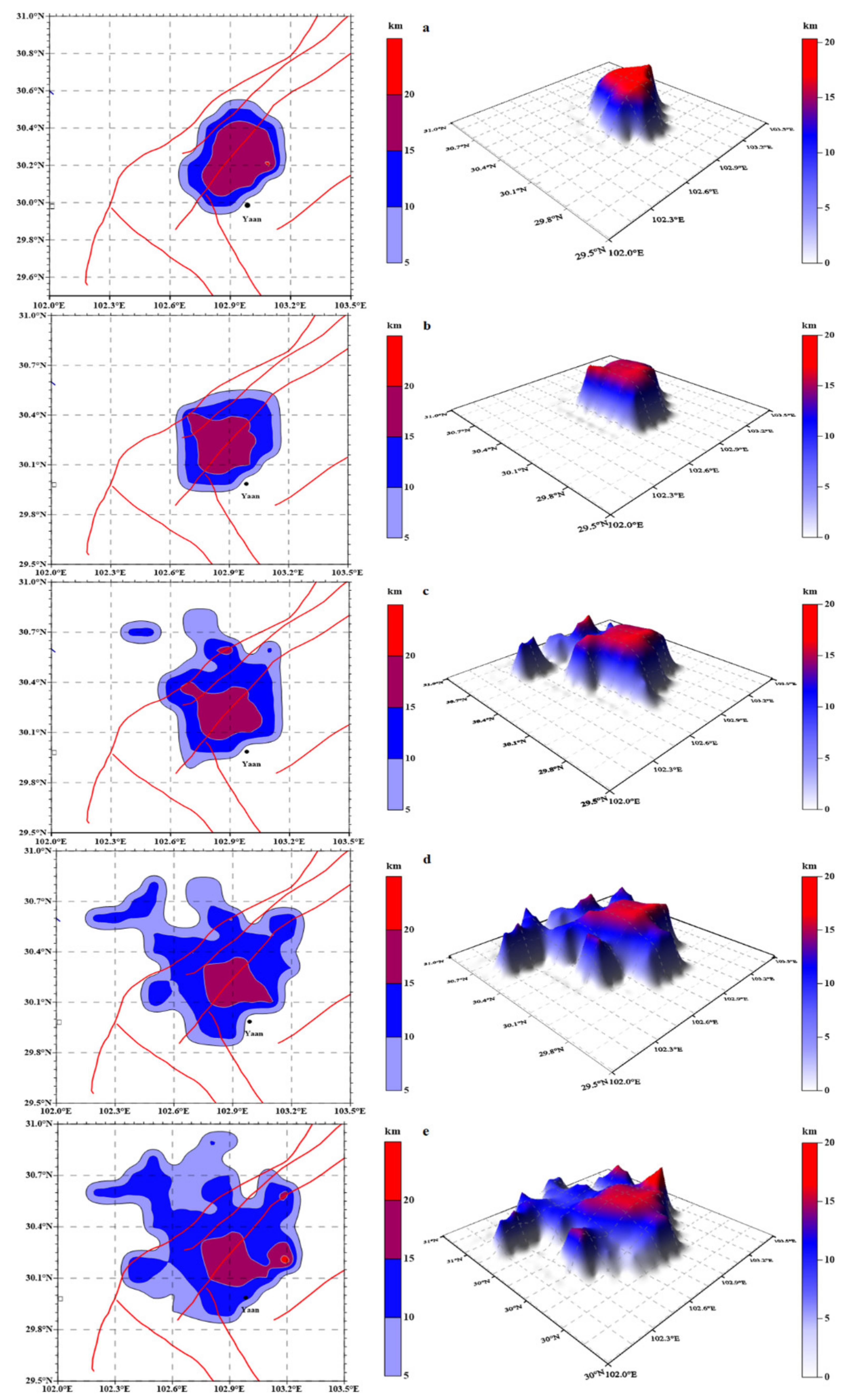
Spatial scanning was performed using events with depth data in the catalog, i.e., at a step size of 0.1° for both longitude and latitude. For all earthquakes in each 0.1° × 0.1° grid point, the average depth was used as the depth value of the grid point, and then kriging interpolation was applied to all the grids. We counted at least ten events in each grid node in the Wenchuan aftershock zone as samples (as well as five events for the Lushan aftershock zone) to prevent the average depth of grid points from being affected by too few events. The contour lines of depth distribution at different periods after the mainshock were obtained and superimposed with regional faults (Figure 6 and Figure 7).
To illustrate the evolution of the deep seismogenic environment in the Wenchuan aftershock zone. Figure 6 shows the spatial evolution of the aftershock depth at one day, one week, one month, six months, one year, and three years after the mainshock. The analysis shows that the focal depth of the Wenchuan aftershock zone spread along the direction of the fault. With Mianyang as the boundary, the aftershock zone can be divided into the southern section and the northern section. The depth distribution is generally deep in the southeast and shallow in the northwest, and the average aftershock focal depth is 10–15 km.
A comparison of the aftershock activity images depicted by the focal depth information shown in Figure 6d,e revealed that the image formed one year after the mainshock did not show a significantly different pattern in the following two years. This finding indicates that after the mainshock, the aftershock frequency tends to be stable one year later, which means that the active aftershock period of the Wenchuan MS 8.0 was less than one year.
Figure 7 shows the spatial evolution of aftershock depths at one day, one week, five months, ten months, one year and three years after the mainshock in the Lushan aftershock zone. The analysis shows that the focal depths of the Lushan aftershock are distributed around the fault, with the fault as the boundary, with a trend of deep in the southeast and shallow in the northwest. Moreover, a comparison of the regional aftershock activity images depicted by the focal depth information in Figure 7d,e revealed that the pattern of the image formed ten months after the mainshock presented limited changes in the following one year, which indicates that the aftershock frequency tended to be stable ten months after the Lushan mainshock. Therefore, the active aftershock period of the Lushan MS 7.0 earthquake was less than ten months.

5. Discussion

Earthquake interaction can change the stress state of faults, which is reflected in both earthquake activity rate and earthquake size distribution. The relationship between stress state and b value can be used to quantify the effect of large earthquakes that can significantly change the stress states and, therefore, the earthquake size distribution. In contrast to previous studies on the Wenchuan and Lushan earthquakes, our paper focuses on a quantitative analysis and discussion of the effect of the Wenchuan MS 8.0 and Lushan MS 7.0 earthquakes on the size distribution of the earthquakes along the Longmenshan fault at different times.
Interpretation of the b value and its variability according to physical mechanisms has received considerable attention and discussion. In most cases, the observation of spatial and temporal b value variability can be caused by several factors: (i) Process of estimation: homogeneity of catalog and method of calculation can affect the results. All the data in this work are from the Longmenshan fault and its surroundings, and each event includes the time, location and magnitude depth. The maximum likelihood estimation and least-squares regression method [30,41,42,43,52,53,54,55] are used to estimate the b value and its uncertainty, but the latter is excessively affected by the largest earthquake magnitude. Marzocchi et al. [56] measured the bias on b values caused by the magnitude binning and catalog incompleteness when the b value is estimated by the maximum likelihood estimation and provided guidance to reduce the likelihood of being misled by b value variation. (ii) Stress conditions: the b value and its variation represent stress buildup and release. The differential stress is inversely dependent on the b value has been observed in laboratory experiments [57,58] as well as in the field [59,60]. The stress acting on a fault may control the variation in the b value in space and time. Parsons et al. [61] calculated the regional Coulomb stress changes on major faults surrounding the rupture resulting from the Wenchuan MS 8.0 and showed that significant stress increased in the Lushan aftershock zone. Other studies obtained similar results [5,6,62]. The spatial variation in the b values throughout the Lushan aftershock zone decreased after the MS 8.0 mainshock (Figure 5i), and the same effect occurred in the southern part of the Wenchuan aftershock zone after the MS 7.0 event (Figure 5g). These findings suggest that the b value is negatively correlated with stress and indicate the effect of the earthquake interaction along the Longmenshan fault zone. (iii) Crustal tectonics: the variation in b value can be interpreted according to the tectonic characteristics, i.e., rock heterogeneity [63], focal depth [23], pore pressure [26], and fault types [24,25]. Previous studies have shown that the b value in different types of faults is b (normal) > 1, b (strike-slip)~1, and b (thrust) < 1 [26,64]. As shown in the spatial footprints in Figure 5, the b value of the southern part of the Longmenshan fault zone is lower than that in the northern part. This pattern is consistent with the tectonic characteristics of the Longmenshan fault, which is a strike-slip fault in the north and a thrust fault in the southern part [65,66].
Stress changes seem to be a key factor that affects the b value and its variation. Excepting the approach of estimation, all other factors are secondary because they are directly or indirectly affected by the stress [67]. Therefore, the observed falls in the b values shown in Figure 5a,b was interpreted as changes in the related stress conditions, which could be precursors to large earthquakes. However, these temporal variations may occur over a timescale ranging from months to years, and the timeliness and effectiveness of this variability as an indicator are difficult to guarantee. Additionally, there is usually an insufficient number of events to accurately calculate the b value before large earthquakes. Gulia and Wiemer [41] pointed out that the period following a moderate earthquake is rich in such data, with thousands of events occurring within a short period. These events may allow real-time monitoring of the evolution of b values. The authors claim that the probability of a larger earthquake following a moderate earthquake increases by several orders of magnitude if the b value remains the same or drops significantly rather than increases. However, Brodsky [68] suggested that the observed pattern revealing the changes in b values is a statistical effect rather than deterministic and that researchers need more cases to test this claim.
In general, thousands of aftershocks occur in the period following a large earthquake. Based on these abundant data, there are two typically common operational aftershock forecasting models used in aftershock hazard assessment, namely the short-term earthquake probability (STEP) model [69] and epidemic-type aftershock sequence model [14,15]. Gulia et al. [16] reported that these models forecast a high probability for a repeat of the mainshock rupture and thus substantially overestimate the aftershock hazard. This paradox can be resolved by taking into account the stress changes and their effect on the earthquake size distribution.
Our results showed that the time series of the b value in the Longmenshan fault zone after the mainshocks exhibited a period of significant fluctuation before returning to the stable state in both the Wenchuan aftershock zone (one year) and the Lushan aftershock zone (ten months). Figure 6 and Figure 7 show that the time required for the b values to return to a stable state after both mainshocks was entirely consistent with the time required for the aftershock depth images to cease changing visibly. The spatial footprints of the changes in the b value reveal that the southern part of the Longmenshan fault zone is lower than the northern part. This finding demonstrates that the Wenchuan and Lushan events did not change the pattern of higher stress in the southern part of the Longmenshan fault zone than in the northern part. However, the most obvious change is that after the mainshock, the size distribution of the subsequent earthquakes in the Wenchuan source region shifts toward relatively larger events (lower b values).
The Longmenshan fault zone began to develop in the Late Triassic, and severe tectonic deformation occurred during the Indo-China and Himalayan movements, forming a combination of thrust and strike-slip displacement [66,70]. Previous studies did not comprehensively quantify the stable state for the Longmenshan fault zone before and after the two large events in a long time series [5,6,27,29,30,55,71]. The b value is a measurable indicator of earthquake size distribution within a specified region and period of time and is dependent on stress. With our present results, we reported the temporal and spatial variation in b values before and after two big earthquakes and fitted the source depth in time and space to quantify the stress changes and their effect on the earthquake size distribution in the Longmenshan fault zone.

6. Conclusions

Based on the tectonic characteristics and potential seismicity surrounding the aftershock zones of the Wenchuan MS 8.0 and Lushan MS 7.0 earthquakes, we studied the spatial and temporal variation of b values in two source regions from 2000 to 2019. In addition, the spatial evolution process of the deep seismogenic environment in the Wenchuan and Lushan aftershock zones was drawn by spatial scanning and depth data fitting.
The results depict the decreasing trends of b values before the two large earthquakes in the study region. Additionally, the b value in the Wenchuan aftershock zone took approximately one year to enter a new stable state (b values ranging from 1.21 to 0.84), while the b value in the Lushan aftershock zone took approximately ten months to return to its original stable state (b = 0.76). Moreover, the major aftershock active periods of the Wenchuan MS 8.0 and Lushan MS 7.0 earthquakes were less than one year and ten months, respectively, which are consistent with the time required for the b value to return to a stable state. The spatial footprints of the changes in the b values results reveal that the Wenchuan MS 8.0 and Lushan MS 7.0 events did not change the pattern of high b values in the north and low b values in the south along the Longmenshan fault zone.
We quantified the effect of the Wenchuan MS 8.0 and Lushan MS 7.0 earthquakes on the size distribution of earthquakes along the Longmenshan fault. Future studies can focus on how to quantify the effect of large earthquake size distribution across different tectonic regimes and apply the findings in potential seismic risk assessment.

Author Contributions

Conceptualization, C.H., C.C. and P.G.; Data curation, P.G. and J.Y.; Formal analysis, C.H.; Funding acquisition, S.S.; Investigation, S.S.; Methodology, S.S. and J.C.; Resources, C.C.; Software, J.C., J.Y. and M.Z.; Supervision, P.G.; Validation, P.G. and M.Z.; Visualization, S.S. and M.Z.; Writing–Original draft, C.H.; Writing–Review & editing, C.C. All authors have read and agreed to the published version of the manuscript.

Funding

This research was supported by the National Natural Science Foundation of China (Grant No. 41771537) and the Fundamental Research Funds for the Central Universities.

Data Availability Statement

Datasets for this research are available in these in-text data citation references: Shi et al. (2018), [http://doi.org/10.6038/cjg2018M0024], Li et al. (2018), [http://doi.org/10.6038/cjg2018M0129] and China Earthquake Networks Center (CENC), [http://www.cenc.ac.cn/].

Acknowledgments

The authors thank American Journal Experts (AJE) for polishing the language of this article.

Conflicts of Interest

No conflict of interest exist in the submission of this manuscript, and the manuscript is approved by all authors for publication.

References

  1. Jia, K.; Zhou, S.; Zhuang, J.; Jiang, C. Possibility of the independence between the 2013 Lushan earthquake and the 2008 Wenchuan earthquake on Longmen Shan fault, Sichuan, China. Seismol. Res. Lett. 2014, 85, 60–67. [Google Scholar] [CrossRef] [Green Version]
  2. Zhang, Y.Q.; Dong, S.W.; Hou, C.T.; Shi, J.S.; Wu, Z.H.; Li, H.L.; Sun, P.; Liu, G.; Li, J. Seismogenic structure of the April 20, 2013, Lushan Ms7 earthquake in Sichuan. Acta Geol. Sin. Engl. Ed. 2013, 87, 633–645. [Google Scholar]
  3. Li, Y.Q.; Jia, D.; Wang, M.M.; Shaw, J.H.; He, J.K.; Lin, A.M.; Xiong, L.; Rao, G. Structural geometry of the source region for the 2013 Mw 6.6 Lushan earthquake: Implication for earthquake hazard assessment along the Longmen Shan. Earth Planet. Sci. Lett. 2014, 390, 275–286. [Google Scholar] [CrossRef]
  4. Du, F.; Long, F.; Ruan, X.; Yi, G.X.; Wu, J. The M7.0 Lushan earthquake and the relationship with the M8.0 Wenchuan earthquake in Sichuan, China. Chin. J. Geophys. 2013, 56, 1772–1783. [Google Scholar]
  5. Parsons, T.; Segou, M. Stress, distance, magnitude, and clustering influences on the success or failure of an aftershock forecast: The 2013 M 6.6 Lushan earthquake and other examples. Seismol. Res. Lett. 2014, 85, 44–51. [Google Scholar] [CrossRef]
  6. Zhu, S. Is the 2013 Lushan earthquake (Mw = 6.6) a strong aftershock of the 2008 Wenchuan, China mainshock (Mw= 7.9)? J. Geodyn. 2016, 99, 16–26. [Google Scholar] [CrossRef]
  7. Toda, S.; Stein, R.S.; Lin, J. Widespread seismicity excitation throughout central Japan following the 2011 M= 9.0 Tohoku earthquake and its interpretation by Coulomb stress transfer. Geophys. Res. Lett. 2011, 38. [Google Scholar] [CrossRef] [Green Version]
  8. Wedmore, L.; Walker, J.F.; Roberts, G.P.; Sammonds, P.; McCaffrey, K.; Cowie, P. A 667 year record of coseismic and interseismic Coulomb stress changes in central Italy reveals the role of fault interaction in controlling irregular earthquake recurrence intervals. J. Geophys. Res. Solid Earth 2017, 122, 5691–5711. [Google Scholar] [CrossRef] [Green Version]
  9. Verdecchia, A.; Pace, B.; Visini, F.; Scotti, O.; Peruzza, L.; Benedetti, L. The role of viscoelastic stress transfer in long-term earthquake cascades: Insights after the central Italy 2016–2017 seismic sequence. Tectonics 2018, 37, 3411–3428. [Google Scholar] [CrossRef] [Green Version]
  10. Kilb, D.; Gomberg, J.; Bodin, P. Aftershock triggering by complete Coulomb stress changes. J. Geophys. Res. Solid Earth 2002, 107, ESE 2-1–ESE 2-14. [Google Scholar] [CrossRef]
  11. Toda, S.; Stein, R.S.; Beroza, G.C.; Marsan, D. Aftershocks halted by static stress shadows. Nat. Geosci. 2012, 5, 410–413. [Google Scholar] [CrossRef]
  12. DeVries, P.M.; Viégas, F.; Wattenberg, M.; Meade, B.J. Deep learning of aftershock patterns following large earthquakes. Nature 2018, 560, 632–634. [Google Scholar] [CrossRef] [PubMed]
  13. Utsu, T.; Ogata, Y. The centenary of the Omori formula for a decay law of aftershock activity. J. Phys. Earth 1995, 43, 1–33. [Google Scholar] [CrossRef]
  14. Ogata, Y. Statistical models for earthquake occurrences and residual analysis for point processes. J. Am. Stat. Assoc. 1988, 83, 9–27. [Google Scholar] [CrossRef]
  15. Ogata, Y. Space-time point-process models for earthquake occurrences. Ann. Inst. Stat. Math. 1998, 50, 379–402. [Google Scholar] [CrossRef]
  16. Gulia, L.; Rinaldi, A.; Tormann, T.; Vannucci, G.; Enescu, B.; Wiemer, S. The Effect of a Mainshock on the Size Distribution of the Aftershocks. Geophys. Res. Lett. 2018, 45, 13277–13287. [Google Scholar] [CrossRef] [Green Version]
  17. Gutenberg, B.; Richter, C.F. Frequency of earthquakes in California. Bull. Seismol. Soc. Am. 1944, 34, 185–188. [Google Scholar] [CrossRef]
  18. Wech, A.G.; Creager, K.C.; Houston, H.; Vidale, J.E. An earthquake-like magnitude-frequency distribution of slow slip in northern Cascadia. Geophys. Res. Lett. 2010, 37. [Google Scholar] [CrossRef] [Green Version]
  19. El-Isa. Continuous-cyclic variations in the b-value of the earthquake frequency-magnitude distribution. Earthquake Science 2013, 26(5), 301–320. [Google Scholar] [CrossRef] [Green Version]
  20. Nuannin, P.; Kulhanek, O.; Persson, L. Spatial and temporal b value anomalies preceding the devastating off coast of NW Sumatra earthquake of December 26, 2004. Geophys. Res. Lett. 2005, 32. [Google Scholar] [CrossRef]
  21. Amitrano, D. Brittle-ductile transition and associated seismicity: Experimental and numerical studies and relationship with the b value. J. Geophys. Res. Solid Earth 2003, 108. [Google Scholar] [CrossRef] [Green Version]
  22. Goebel, T.H.W.; Schorlemmer, D.; Becker, T.W.; Dresen, G.; Sammis, C.G. Acoustic emissions document stress changes over many seismic cycles in stick-slip experiments. Geophys. Res. Lett. 2013, 40, 2049–2054. [Google Scholar] [CrossRef] [Green Version]
  23. Spada, M.; Tormann, T.; Wiemer, S.; Enescu, B. Generic dependence of the frequency-size distribution of earthquakes on depth and its relation to the strength profile of the crust. Geophys. Res. Lett. 2013, 40, 709–714. [Google Scholar] [CrossRef] [Green Version]
  24. Schorlemmer, D.; Wiemer, S.; Wyss, M. Variations in earthquake-size distribution across different stress regimes. Nature 2005, 437, 539. [Google Scholar] [CrossRef]
  25. Gulia, L.; Wiemer, S. The influence of tectonic regimes on the earthquake size distribution: A case study for Italy. Geophys. Res. Lett. 2010, 37. [Google Scholar] [CrossRef]
  26. Bachmann, C.E.; Wiemer, S.; Goertz-Allmann, B.; Woessner, J. Influence of pore-pressure on the event-size distribution of induced earthquakes. Geophys. Res. Lett. 2012, 39. [Google Scholar] [CrossRef] [Green Version]
  27. Zhao, Y.; Wu, Z. Mapping the b-values along the Longmenshan fault zone before and after the 12 May 2008, Wenchuan, China, Ms 8.0 earthquake. Nat. Hazards Earth Syst. Sci. 2008, 8, 1375–1385. [Google Scholar] [CrossRef] [Green Version]
  28. Zhang, S.; Zhou, S. Spatial and temporal variation of b-values in southwest China. Pure Appl. Geophys. 2016, 173, 85–96. [Google Scholar] [CrossRef]
  29. Liu, Y.; Pei, S.; Pei, S. Temporal and spatial variation of b-value before and after Wenchuan earthquake and its tectonic implication. Chin. J. Geophys. 2017, 60, 2104–2112. [Google Scholar]
  30. Shi, H.X.; Meng, L.Y.; Zhang, X.M.; Chang, Y.; Yang, Z.T.; Xie, W.Y.; Hattori, K.; Han, P. Decrease in b value prior to the Wenchuan earthquake (M(s) 8.0). Chin. J. Geophys. Chin. Ed. 2018, 61, 1874–1882. [Google Scholar]
  31. Zhao, B.; Yang, G.; Wang, J.; Dong, F. Research on b-Values Based on Fault Buffers. Pure Appl. Geophys. 2020, 177, 71–80. [Google Scholar] [CrossRef]
  32. Stein, R.S.; Barka, A.A.; Dieterich, J.H. Progressive failure on the North Anatolian fault since 1939 by earthquake stress triggering. Geophys. J. Int. 1997, 128, 594–604. [Google Scholar] [CrossRef] [Green Version]
  33. Mallman, E.P.; Zoback, M.D. Assessing elastic Coulomb stress transfer models using seismicity rates in southern California and southwestern Japan. J. Geophys. Res. Solid Earth 2007, 112. [Google Scholar] [CrossRef] [Green Version]
  34. Delescluse, M.; Chamot-Rooke, N.; Cattin, R.; Fleitout, L.; Trubienko, O.; Vigny, C. April 2012 intra-oceanic seismicity off Sumatra boosted by the Banda-Aceh megathrust. Nature 2012, 490, 240–244. [Google Scholar] [CrossRef]
  35. Durand, V.; Bouchon, M.; Karabulut, H.; Marsan, D.; Schmittbuhl, J. Link between Coulomb stress changes and seismic activation in the eastern Marmara sea after the 1999, Izmit (Turkey), earthquake. J. Geophys. Res. Solid Earth 2013, 118, 681–688. [Google Scholar] [CrossRef]
  36. Sumy, D.F.; Cochran, E.S.; Keranen, K.M.; Wei, M.; Abers, G.A. Observations of static Coulomb stress triggering of the November 2011 M5. 7 Oklahoma earthquake sequence. J. Geophys. Res. Solid Earth 2014, 119, 1904–1923. [Google Scholar] [CrossRef]
  37. Zuniga, F.R.; Wyss, M. Most-and least-likely locations of large to great earthquakes along the Pacific coast of Mexico estimated from local recurrence times based on b-values. Bull. Seismol. Soc. Am. 2001, 91, 1717–1728. [Google Scholar] [CrossRef] [Green Version]
  38. Nanjo, K.; Hirata, N.; Obara, K.; Kasahara, K. Decade-scale decrease in b value prior to the M9-class 2011 Tohoku and 2004 Sumatra quakes. Geophys. Res. Lett. 2012, 39. [Google Scholar] [CrossRef]
  39. Woessner, J.; Wiemer, S. Assessing the quality of earthquake catalogues: Estimating the magnitude of completeness and its uncertainty. Bull. Seismol. Soc. Am. 2005, 95, 684–698. [Google Scholar] [CrossRef]
  40. Mignan, A.; Werner, M.J.; Wiemer, S.; Chen, C.C.; Wu, Y.M. Bayesian estimation of the spatially varying completeness magnitude of earthquake catalogs. Bull. Seismol. Soc. Am. 2011, 101, 1371–1385. [Google Scholar] [CrossRef]
  41. Gulia, L.; Wiemer, S. Real-time discrimination of earthquake foreshocks and aftershocks. Nature 2019, 574, 193–199. [Google Scholar] [CrossRef] [PubMed]
  42. Aki, K. Maximum likelihood estimate of b in the formula log N = a-bM and its confidence limits. Bull. Earthq. Res. Inst. Tokyo Univ. 1965, 43, 237–239. [Google Scholar]
  43. Utsu, T. A method for determining the value of “b” in a formula log n = a-bM showing the magnitude-frequency relation for earthquakes. Geophys. Bull. Hokkaido Univ. 1965, 13, 99–103. [Google Scholar]
  44. Tormann, T.; Wiemer, S.; Mignan, A. Systematic survey of high-resolution b value imaging along Californian faults: Inference on asperities. J. Geophys. Res. Solid Earth 2014, 119, 2029–2054. [Google Scholar] [CrossRef]
  45. Akaike, H. A new look at the statistical model identification. In Selected Papers of Hirotugu Akaike; Springer: Berlin/Heidelberg, Germany, 1974; pp. 215–222. [Google Scholar]
  46. Utsu, T. Report of the Joint Research Institute for Statistical Mathematics; Institute for Statistical Mathematics; Tokyo, Japan, 1992. [Google Scholar]
  47. Utsu, T. Representation and analysis of the earthquake size distribution: A historical review and some new approaches. Pure Appl. Geophys. 1999, 155, 509–535. [Google Scholar] [CrossRef]
  48. McGrath, D.; Zhang, C.; Carton, O.T. Geostatistical analyses and hazard assessment on soil lead in Silvermines area, Ireland. Environ. Pollut. 2004, 127, 239–248. [Google Scholar] [CrossRef]
  49. Ha, H.; Olson, J.R.; Bian, L.; Rogerson, P.A. Analysis of heavy metal sources in soil using kriging interpolation on principal components. Environ. Sci. Technol. 2014, 48, 4999–5007. [Google Scholar] [CrossRef]
  50. Huang, Q. Seismicity changes prior to the Ms8. 0 Wenchuan earthquake in Sichuan, China. Geophys. Res. Lett. 2008, 35. [Google Scholar] [CrossRef]
  51. Fang, L.; Wu, J.; Wang, W.; Du, W.; Su, J.; Wang, C.; Yang, T.; Cai, Y. Aftershock observation and analysis of the 2013 M S 7.0 Lushan earthquake. Seismol. Res. Lett. 2015, 86, 1135–1142. [Google Scholar] [CrossRef] [Green Version]
  52. Lopez-Pineda, L. and Rebollar, C.J. Source characteristics of the Mw 6.2 loreto earthquake of 12 March 2003 that occurred in a transform fault in the middle of the Gulf of California, Mexico. Bull. Seismol. Soc. Am. 2005, 95, 419–430. [Google Scholar] [CrossRef]
  53. Singh, A.P.; Mishra, O.P.; Rastogi, B.K.; Kumar, D. 3-D seismic structure of the Kachchh, Gujarat, and its implications for the earthquake hazard mitigation. Nat. Hazards 2011, 57, 83–105. [Google Scholar] [CrossRef]
  54. Woessner, J.; Laurentiu, D.; Giardini, D.; Crowley, H.; Cotton, F.; Grunthal, G.; Valensise, G.; Arvidsson, R.; Basili, R.; Demircioglu, M.B.; et al. The 2013 European Seismic Hazard Model: Key components and results. Bull. Earthq. Eng. 2015, 13, 3553–3596. [Google Scholar] [CrossRef] [Green Version]
  55. Li, L.; Adhikari, L.B.; Gang, L.; FuWang, G. Characteristics of temporal-spatial distribution of the aftershocks of the 2008 M(s) 8. 0 Wenchuan Earthquake. Chin. J. Geophys. Chin. Ed. 2018, 61, 1797–1805. [Google Scholar]
  56. Marzocchi, W.; Spassiani, I.; Stallone, A.; Taroni, M. How to be fooled searching for significant variations of the b-value. Geophys. J. Int. 2020, 220, 1845–1856. [Google Scholar] [CrossRef]
  57. Varotsos, P.; Sarlis, N.; Skordas, E.; Lazaridou, M. Seismic Electric Signals: An additional fact showing their physical interconnection with seismicity. Tectonophysics 2013, 589, 116–125. [Google Scholar] [CrossRef]
  58. Sarlis, N.V.; Skordas, E.S.; Varotsos, P.A.; Nagao, T.; Kamogawa, M.; Tanaka, H.; Uyeda, S. Minimum of the order parameter fluctuations of seismicity before major earthquakes in Japan. Proc. Natl. Acad. Sci. USA 2013, 110, 13734–13738. [Google Scholar] [CrossRef] [Green Version]
  59. Scholz, C.H. On the stress dependence of the earthquake b value. Geophys. Res. Lett. 2015, 42, 1399–1402. [Google Scholar] [CrossRef] [Green Version]
  60. Rodriguez-Perez, Q.; Ramon Zuniga, F. Imaging b-value depth variations within the Cocos and Rivera plates at the Mexican subduction zone. Tectonophysics 2018, 734, 33–43. [Google Scholar] [CrossRef]
  61. Parsons, T.; Ji, C.; Kirby, E. Stress changes from the 2008 Wenchuan earthquake and increased hazard in the Sichuan basin. Nature 2008, 454, 509–510. [Google Scholar] [CrossRef]
  62. Shan, B.; Xiong, X.; Zheng, Y.; Jin, B.; Liu, C.; Xie, Z.; Hsu, H. Stress changes on major faults caused by 2013 Lushan earthquake and its relationship with 2008 Wenchuan earthquake. Sci. China-Earth Sci. 2013, 56, 1169–1176. [Google Scholar] [CrossRef]
  63. Gerstenberger, M.; Wiemer, S.; Giardini, D. A systematic test of the hypothesis that the b value varies with depth in California. Geophys. Res. Lett. 2001, 28, 57–60. [Google Scholar] [CrossRef]
  64. Beauval, C.; Scotti, O. Quantifying sensitivities of PSHA for France to earthquake catalog uncertainties, truncation of ground-motion variability, and magnitude limits. Bull. Seismol. Soc. Am. 2004, 94, 1579–1594. [Google Scholar] [CrossRef]
  65. Hubbard, J.; Shaw, J.H. Uplift of the Longmen Shan and Tibetan plateau, and the 2008 Wenchuan (M = 7.9) earthquake. Nature 2009, 458, 194–197. [Google Scholar] [CrossRef] [PubMed]
  66. Lei, J.; Zhao, D. Structural heterogeneity of the Longmenshan fault zone and the mechanism of the 2008 Wenchuan earthquake (Ms 8.0). Geochem. Geophys. Geosystems 2009, 10. [Google Scholar] [CrossRef]
  67. El-Isa, Z.H.; Eaton, D.W. Spatiotemporal variations in the b-value of earthquake magnitude–frequency distributions: Classification and causes. Tectonophysics 2014, 615, 1–11. [Google Scholar] [CrossRef]
  68. Brodsky, E.E. Determining whether the worst earthquake has passed. Nature 2019, 574, 185–186. [Google Scholar] [CrossRef]
  69. Gerstenberger, M.C.; Wiemer, S.; Jones, L.M.; Reasenberg, P.A. Real-time forecasts of tomorrow’s earthquakes in California. Nature 2005, 435, 328. [Google Scholar] [CrossRef]
  70. Deng, B.; Liu, S.G.; Jansa, L.; Cao, J.X.; Cheng, Y.; Li, Z.W.; Liu, S. Sedimentary record of Late Triassic transpressional tectonics of the Longmenshan thrust belt, SW China. J. Asian Earth Sci. 2012, 48, 43–55. [Google Scholar] [CrossRef]
  71. Wang, Y.; Wang, F.; Wang, M.; Shen, Z.-K.; Wan, Y. Coulomb Stress Change and Evolution Induced by the 2008 Wenchuan Earthquake and its Delayed Triggering of the 2013 M-W 6.6 Lushan Earthquake. Seismol. Res. Lett. 2014, 85, 52–59. [Google Scholar] [CrossRef] [Green Version]
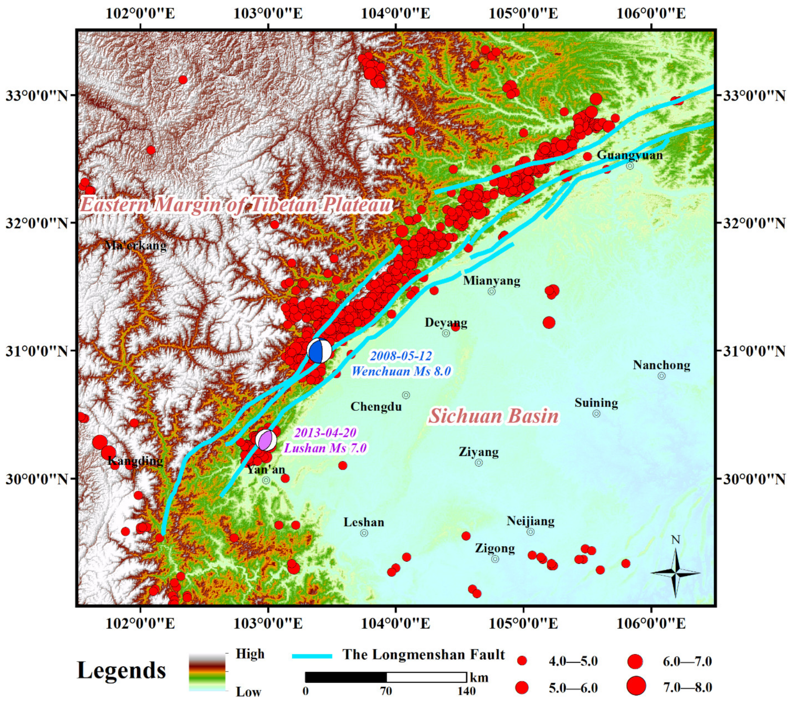
Figure 1. The topographic and tectonic map of the Longmenshan fault zone and its surrounding region. Blue beach ball represents the focal mechanism of the Wenchuan MS 8.0 earthquake. Pink beach ball represents the focal mechanism of the Lushan MS 7.0 earthquake. Red circles represent epicenters of earthquakes (MS ≥ 4) from 1 January 2000 to 1 January 2019.
Applsci 11 08534 g001
Figure 2. Magnitude versus time for events in the Longmenshan fault zone from 2000 to 2019. (a) Magnitude versus time for events in the MS 8.0 Wenchuan source region; (b) magnitude versus time for events in the MS 7.0 Lushan source region.
Applsci 11 08534 g002
Figure 3. Frequency-magnitude distribution of the seismicity of the Wenchuan-Lushan sequence from 1 January 2000 to 1 January 2019.
Applsci 11 08534 g003
Figure 4. Frequency-magnitude distribution and NLIndex.
Applsci 11 08534 g004
Figure 5. Temporal and spatial analysis of the b values for the Wenchuan-Lushan sequence. (a,b) Temporal variation of b values for the Wenchuan and Lushan source regions. The dashed black lines represent the times of the MS 8.0 (Wenchuan) and MS 7.0 (Lushan) events, and the dashed blue lines show the background b values for the Wenchuan and Lushan source regions. The dashed red line represents the b value after the time of the MS 7.0 event (Lushan) for the Wenchuan source region. The shaded regions represent the uncertainties in the b values. (c,d) FMDs for the two aftershock zones in three different periods. (eg) Map showing the spatial footprint of b values for the Wenchuan aftershock zone in three different periods. (hj) Map showing the spatial footprint of b values for the Lushan aftershock zone in three different periods.
Applsci 11 08534 g005
Figure 6. Spatial distribution of the focal depths of the aftershocks following the Wenchuan MS 8.0 earthquake on the fault plane. Red lines represent the locations of faults. (a) One day after the mainshock; (b) 1 week after the mainshock; (c) 1 month after the mainshock; (d) 1 year after the mainshock; and (e) 3 years after the mainshock.
Applsci 11 08534 g006
Figure 7. Spatial distribution of the focal depths of the aftershocks following the Lushan MS 7.0 earthquake on the fault plane. Red lines represent the locations of faults. (a) One day after the mainshock; (b) 1 month after the mainshock; (c) 5 months after the mainshock; (d) 10 months after the mainshock; and (e) 2 years after the mainshock.
Applsci 11 08534 g007
Table 1. Results of the P parameter test between windows.
WindowsΔAICPb
W1 and W22.60.03
W2 andW39.99.5 × 10−4
W1 and W328.97.1 × 10−8
L1 and L22.60.03
L2 and L34.60.01
L1 and L3205.9 × 10−6
Publisher’s Note: MDPI stays neutral with regard to jurisdictional claims in published maps and institutional affiliations.