Abstract
Chilean seismic activity is one of the strongest in the world. As already shown in previous papers, seismic activity can be usefully described by a space–time branching process, such as the ETAS (Epidemic Type Aftershock Sequences) model, which is a semiparametric model with a large time-scale component for the background seismicity and a small time-scale component for the triggered seismicity. The use of covariates can improve the description of triggered seismicity in the ETAS model, so in this paper, we study the Chilean seismicity separately for the North and South area, using some GPS-related data observed together with ordinary catalog data. Our results show evidence that the use of some covariates can improve the fitting of the ETAS model.
1. Introduction
Chile is considered one of the most active seismic countries in the world due to its particular location. In particular, Chile is located on three great tectonic plates: Nazca, South American, and Antarctic. The seismic events in Chile result from the convergence of the oceanic lithosphere of the Nazca plate beneath the South American continental plate at a rate of about 6.5 cm/year [1]. The strong coupling between the two plates produces the most intense seismicity and the largest earthquakes in the country [2,3,4]. Seismic activity induces various types of ground movements, as seismic waves (P and S-waves), which can cause significant damages to structures, and consequently losses of lives [5,6]. The velocity of the waves can be different according to the depth [7,8].
Seismic activity can be described by a spatio-temporal branching process, such as the ETAS (Epidemic Type Aftershock Sequences) model [9], which is a semiparametric model with a large time-scale component for the background seismicity and a small time-scale component for the triggered seismicity. The large-scale component intensity function is usually estimated by nonparametric techniques, specifically in our paper, we used the Forward Likelihood Predictive approach (FLP) approach [10,11,12]; the triggered seismicity is modeled with a parametric space–time function. In classical ETAS models, the expected number of triggered events depends only on the magnitude of the main event. In previous papers [13,14] we already used the classical ETAS model to describe Chilean seismicity, also using different models for different Chilean areas.
From a statistical point of view, forecast of riggered seismicity can be performed in the days following a big event; of course, the estimation of this component is very important to forecast the evolution of a seismic sequence in space and time domain.
In the classical ETAS model [9], the average number of future triggered events just depends on the magnitude of the previous event. Although that represents a very comfortable and useful model, in many situations, it may be too simple to describe the aftershocks dynamics, as often highlighted by diagnostic analysis. Furthermore, the high seismicity of Chile, together with the recent increasing GPS data availability, allowed us to consider a much more complex model for describing and analyzing the Chilean triggered activity. In this paper, we provide a description of the triggered seismicity in Chile after a subdivision of the country into two spatial areas. In particular, based on the methodology proposed by [15], we suggest the use of a specific branching-type model for earthquake description (the ETAS model) in a regression-oriented version, accounting also for external covariates, related to the depth of events and to some GPS measurements. For further examples on applications incorporating the external information in self-exciting models, see [16,17,18,19].
Interesting and encouraging results, though not completely satisfactory, are provided, accounting for covariates related to the depth of events and to some GPS measurements, corresponding to the Earth movement observed until the time of main events. In addition, some of the proposed models can improve the description and the forecasting of the triggeredseismicity in Chile, if compared to the classical ETAS model.
All the reported results are obtained using the open-source software developed in R [20,21].
This paper is organized as follows. In Section 2 a description of data is provided jointly to some preliminary analysis. Section 3 reports some details of the theoretical background, recalling some basic theory of space–time point processes and the ETAS model, with an extension of the FLP approach with the inclusion of covariates. The choice of covariates is described in Section 4. A seismic application to the considered data is discussed in Section 5. Section 6 is devoted to discussion of results. Conclusions are reported in Section 7.
2. Description of the Datasets
In this paper, two datasets are analyzed: the catalog of the Chilean seismic events and the GPS measurements in the area between latitudes [] and longitudes [].
2.1. The Seismic Catalog and Chilean Seismicity
The Chilean catalog has been provided by the Chilean National Seismological Center of the University of Chile (http://sismologia.cl (accessed on 10 February 2021)). It contains the ordinary seismic variables, such as latitude, longitude, magnitude (on the Richter scale), depth, and time of occurrence of each seismic event (year, month, day, hour, minute, and seconds).
From Figure 1, it is observed that the largest number of seismic events occurred in the years 2010, 2014, and 2015, which coincide with the occurrence of the highest magnitude earthquakes, of magnitudes 8.8, 8.2 and 8.4 on the Richter scale, respectively. The relationship between month and magnitude is explicitly represented in Figure 2. From this figure it is also observed that the original seismic data are normally collected with a threshold in the minimum magnitudes, since very low magnitudes are difficult to be detected.
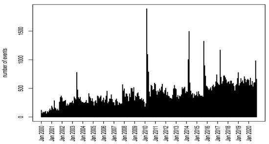
Figure 1.
Distribution of number of events by month in Chile.
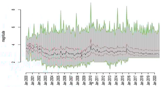
Figure 2.
Magnitude distribution by month; the green lines are the monthly minima and maxima, the red lines are the first and third monthly quartiles, while the black line is the monthly median.
Some summary statistics, related to the historical seismic activities in Chile in the last 21 years, are reported in Table 1. This table shows that 2010 has the maximum number of events (second column) and the maximum magnitude (third column) as well. In the years 2000 and 2011, two seismic events, with the maximum magnitude in two different spatio-temporal locations, occurred.

Table 1.
Summary statistics of the Chilean seismic events from 2000 to 2020.
Since the seismicity has a different behavior along the coast of Chile, due to the different velocity that the Nazca Plate (Figure 3, left panel) is being subducted beneath South America (see, [22]), we considered two distinct areas (see Figure 3, right panel).
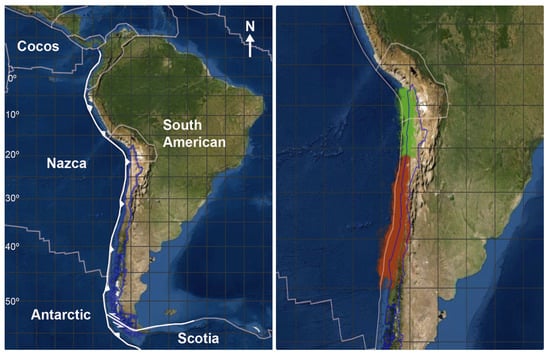
Figure 3.
Left panel: Satellite image of the Southern America, with the evidence of the borders of Chile (in blue) and the tectonic plates (in gray); right panel: seismic events occurred in Chile from 2000 to 2020 in the two studied areas; in green, events in the Northern area and in red, events in the Southern area.
In addition, the considered areas include the major earthquakes of the last 30 years. The Northern area includes the M8.2 Iquique earthquake (2 April 2014) and the second area includes the 2010 Chile earthquake of 8.8 magnitude occurred off the coast of central Chile on Saturday, 27 February 2010, which provoked a rupture of more than 1000 km length, and the M8.4 Coquimbo earthquake occurred on 16 September 2015.
We consider only events with depths less than 70 km in both areas (Figure 4 and Figure 5). Earthquakes deeper than 70 km, which occur within the subducted oceanic lithosphere [8], are excluded in our analysis for both areas. The reason is that the largest earthquakes occur at shallow depths down to 50 km and near the limit of the intermediate-depth seismic segment at 60–70 km [1], beneath the forearc section of the convergent margin. Additionally, most seismic events in Chile occur at depths between 30 and 40 km (Figure 4 and Figure 5). These are mainly due to the deformations generated by the convergence between the Nazca Plate and the continental plate. These deformations caused the rise of the Andes Mountains, and they can reach magnitudes greater than 7 [22].
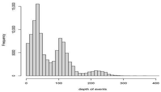
Figure 4.
Distribution of events depths in whole Chile.
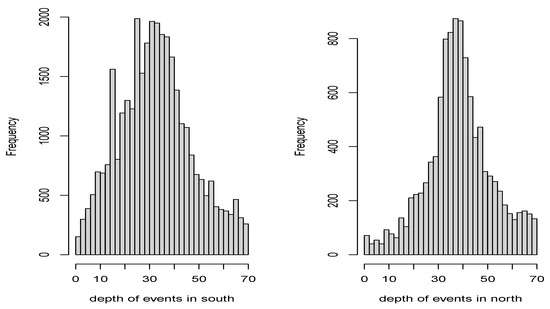
Figure 5.
Distribution of depths of the selected events in the Southern and Northern areas.
The threshold magnitude for the ETAS model, i.e., the lower bound for which earthquakes with higher values of magnitude are surely recorded in the catalog, is obtained by analyzing the log-cumulate distribution of the magnitudes recorded in the two areas (see, Figure 6).
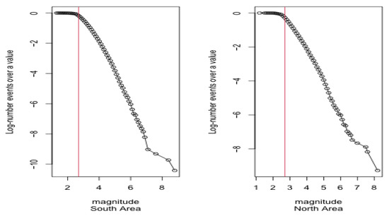
Figure 6.
Log-cumulate distribution of magnitude in the Southern area (on the left) and in the Northern area (on the right).
Based on this information, a value of magnitude is taken as the threshold magnitude for both areas. Starting from an empirical completeness analysis of the catalogs before 2006, events before that date are not identified with the same completeness magnitude. Therefore, only events from 2006 are considered in the proposed study [13,14].
The estimated b-values are 0.586 for the North zone and 0.542 for the Southern one, with standard errors 0.0104 and 0.0050, respectively.
2.2. The GPS Measurements
For calculating the daily accumulated displacements associated with seismic events, we use the GPS measurements (longitude, latitude and altitude above sea level, a.s.l.), downloaded by the website http://geodesy.unr.edu/NGLStationPages/GlobalStationList (accessed on 22 February 2021).
Figure 7 represents the daily coordinates of a GPS station (which name is EMAT) located in the Coquimbo region in the period 2005-2020. The calculation of the accumulated daily horizontal displacements is performed using the GPS measurements of both one day and five days prior to the seismic event, collected by the GPS station closest to the same event. For this calculation, the Euclidean distance, given by , is used. The GPS altitude component, normally used for evaluating the vertical displacement, has not been considered in this application. As documented in various studies, this variable does not have sufficient accuracy, and it is not largely used to describe seismic events [23,24]. Therefore, in the proposed analysis we have not included this variable as potential covariate.
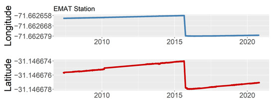
Figure 7.
Time series of the GPS measurements in the EMAT station: longitude (top) and latitude (bottom).
To acquire the accumulated displacements (called Mt1D and Mt5D, for one and five days, respectively) the data were pre-processed by interpolating the missing values using the R package imputTS, [25], and denoising them through the R package wmtsa [26].
3. Branching Point Processes and ETAS Model
Branching processes are used to model reproduction phenomena. These models have been recently considered for the description of different application fields: biology [27], demography [28], epidemiology [29,30].
Any analytic spatio-temporal point process is uniquely characterized by its associated conditional intensity function (CIF) [31] that represents the instantaneous rate or hazard for events at time t and location given all the observations up to time t, conditioning on the random past history of the process .
The conditional intensity function of the branching model is defined as the sum of a term describing the large time- scale variation (spontaneous activity or background) and one relative to the small time-scale variation due to the interaction with the events in the past (triggered activity or offspring):
with , the vector of parameters of the triggered intensity () together with the parameter of the background general intensity (), the space density, and the triggered intensity, given by:
where is the space–time intensity at triggered by a previous event at time . The self-exciting component of the model basically provides a description of the intensity at a space–time location caused by each previous event.
As introduced above, a branching process for earthquake description, widely used in seismological context is the Epidemic Type Aftershocks-Sequences (ETAS) model [9].
The ETAS conditional intensity function can be written, starting from model (1), as follows:
where is the space density of the background/long term component, stationary in time. The aftershock (triggered) component is the product of the density of aftershocks in time, i.e., the Omori law representing the occurrence rate of aftershocks at time t, following the earthquake of time and magnitude , and the density of aftershocks in space. In particular, is the magnitude of the j-th event and the threshold magnitude, k is a normalizing constant, characteristic parameters of the seismic activity of the given region; p is useful for characterizing the pattern of seismicity, indicating the decay rate of aftershocks in time; d and q are two parameters related to the spatial influence of the mainshock. For the spatial triggered distribution, conditioned to magnitude of the generating event, the distribution is:
relating the occurrence rate of aftershocks to the mainshock magnitude , through the parameters that measure the influence on the relative weight of each sequence.
The FLP approach, which is a nonparametric estimation procedure based on the subsequent increments of log-likelihood obtained by adding an observation one at a time, to account for the information of the observations until on the next one, has been developed for estimating the background component [11,32].
The package etasFLP [11,33,34] provides tools to implement this mixed approach for a wide class of ETAS models for the description of seismic events, developed in an R environment [20].
ETAS Model with Covariates
The ETAS model is widely used in the framework of statistical modeling of earthquake occurrence; however, in some applications, it may not adequately describe the triggered seismicity. In the classical ETAS model formulation, as in Equation (2), the average number of events triggered by an event at time depends only on its magnitude . Ref. [15] proposed an ETAS model with covariates in the framework of the survival analysis. This model relates the average number of events triggered by an event at time with the value of some covariates, including magnitude, corresponding to the th event. From a statistical point of view, the inclusion of new explanatory variables can significantly improve the fitting of the model to real observed data.
These variables may also vary continuously in space, and their effect is incorporated in the triggering part of the model. The background component of the model is estimated using the Forward Likelihood for Prediction (FLP) approach [10,11,12].
As proposed by [35] in a context of infection occurrences, in [15] we incorporate the space–time phenomenological laws of the triggering part of the ETAS model with the effects of covariates. In particular, we model the covariates of the ETAS model as in a GLM framework, such that is a classical linear predictor given by , where is the vector of covariates observed for the j-th event and is a vector of unknown parameters. Therefore, the triggering function is factorized into separate effects of marks, time, and relative location:
where is the time and location of individual occurrence j, is a linear predictor, with the external known covariate vector, including the magnitude (usually coinciding with the first covariate), acting in a multiplicative fashion on the base risk and , with a k component vector, to be estimated.
More in details, in the usual ETAS model [9,36], , and . In this model formulation, for an easier correspondence with the ETAS parametrization, in the vector a constant term is not included, since the presence of the parameter in the model.
In the seismic context, that would provide a more general formalism for the earthquake occurrence in space and time. Indeed, the main idea is that the effect on the future activity depends not only on the closeness of the previous events but also on other characteristics of the main event, such as magnitude, as usual, and the distance from the faults, or other geological sources.
An extended version of the package etasFLP for generalized offspring component is available at the CRAN [21].
4. Choosing the Covariates in the ETAS Model Applied to Chile Seismicity
First analysis conducted on Chile catalogs, showed that probably the use of covariates could have improved the performance of the model. Possible choices have also been encouraged by the availability of GPS measurements, which were supposed to be useful in the explanation of triggered seismicity. To explain the intensity of the triggered seismicity, we estimated several models with different sets of covariates, in addition to the magnitude.
In particular, the suitable covariates in both the areas are chosen based on a forward selection strategy: starting from the model with the first covariate magnitude, further covariates are added one by one, and the gain in terms of the Akaike Information Criterion (AIC) is computed. Since the best gain in the AIC values is obtained by adding the variable depth z, it is the second variable introduced in the model. Then, a third variable, chosen from the remaining candidate covariates, is added, and the gain computed. The best result is obtained with the variable Mt5D, which is the third covariate introduced in the model for aftershocks. As a final step, a fourth covariate, Mt1D, gives some further improvement in the AIC value. No further covariates lead to appreciable improvements in terms of AIC.
The ranking and the order of inclusion of the covariates, in the triggered seismicity component, is the same in both the areas, even with different estimated parameters. Then, the selected covariates are: magnitude, z, Mt5D, Mt1D.
5. Results
The two models used in the analyzed areas differ just for the estimation of the parameter p. Indeed, a first procedure for both the areas is carried out with a fixed value of p, very close to 1. However, for the Northern area, the estimation of p leads to a value very close to (but significantly different from) 1.
In Figure 8 the profile log-likelihood for the parameter p is reported for the Northern area. The AIC of the model estimating also p is sensibly lower than the AIC value of the model with p taken as fixed.
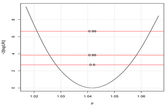
Figure 8.
Profile likelihood for p in Northern area.
Conversely, in the Southern area, the value of p is not significantly different from 1, and the best AIC value is obtained in the model with p fixed to a value very close to 1.
5.1. Comparison of the AIC Values for the Two Areas
The AIC values for the four models fitted to the data of the Northern catalog, with valid observations, are reported in Table 2. The first column reports the AIC values obtained when p is estimated together with other parameters, while the AIC values of the second columns are obtained from models in which p is fixed to . The gain in the AIC values is evident in models with p estimated from the data.
Table 2.
AIC values. North catalog, p estimated.
Similar AIC values for Southern area () are reported in Table 3. Here, evidence is generally in favor of a fixed value of p, especially for the model with three and four covariates, as already seen from the profile likelihood plot (Figure 8).
Table 3.
AIC values. South catalog, p estimated.
The model with four covariates seems to perform better than the simpler models both for the North and South areas.
No further covariates are introduced because no improvement in terms of AIC is observed.
Again, the big gain in terms of AIC is obtained at the second step, with the introduction of z (the depth) in the model for triggered seismicity. However, the main contribution is always given by the magnitude.
5.2. Comparison of Results in the Two Chilean Zone
For the triggered components for the Northern area, according to the AIC values reported in the previous tables, we use as covariates, besides the magnitude, the depth, Mt1D and Mt5D (see estimation results in Table 4). The parameter p is estimated from data.
Table 4.
Estimates and standard error for the ETAS model with four covariates for the Northern area.
For the triggered components for the Southern area, according to the AIC values reported in the previous tables, we consider, besides the magnitude, the same set of covariates used for the Northern area, i.e., the depth, Mt1D and Mt5D (see estimation results in Table 5). p is kept fixed, since no gain in terms of AIC is observed.
Table 5.
Estimates and standard error for the ETAS model with four covariates for the Southern area.
6. Discussion of Results
The obtained results suggest that from a simple AIC point of view, models with four covariates must be preferred for both areas, as already underlined in Section 5.1. Moreover, the estimated parameters differently characterize the two areas, as shown in Table 4 and Table 5 (note for instance the different sign of the variable Mt1D), reflecting the different behavior of the seismicity along the Chilean coast.
However, we report a diagnostic residual plot to see how the four-covariates models perform well. In general, in diagnostic analysis, if the estimated model is a good approximation of the real model that describes data, then the transformed observations (moving each point on the integrated intensity function) should behave like a homogeneous Poisson process [37]. Deviations from it are caused by some characteristics of data not taken into account by the fitted model.
Therefore, in Figure 9 we report the transformed time residual plots for the Northern area, on the left, and for the Southern area, on the right. In both plots, we draw in red the theoretical line (if the model is estimated correctly), in black the line for the transformed residuals obtained fitting an ETAS model with four covariates, and finally in green the line of the transformed residuals fitting the classical ETAS model. From the left panel of Figure 9 it is clear that the four-covariates model can describe the triggering behaviors in the Northern area. Nevertheless, the black and green lines on the right panel of Figure 9 related to the South area are very close to each other, showing that probably the fitted four-covariates ETAS model does not fully describe the complex triggering mechanism of the Southern area.
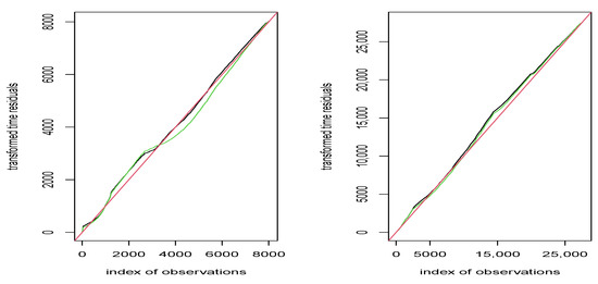
Figure 9.
Transformed residuals obtained from the model with four covariates (black line) and one covariate (green line), for the Northern area (left panel) and the Southern Area (right panel). The red line is the theoretical one.
7. Conclusions
In this paper, we present an application of the ETAS model with covariates to describe the Chilean seismicity, also using GPS information of the observed data. In particular, the triggered seismicity in Chile is analyzed distinguishing between the North and the South of the country, since the different behavior of the seismicity along the coast of Chile. According to the analyzed areas, different results are obtained, accounting for the main relevant covariates related to the depth of events and some GPS measurements, corresponding to the Earth movement observed until the time of main events. It represents an innovative method, improving the assessment of seismic events in space and time, considering a contagion model within a regression-like framework accounting for external covariates. Moreover, the introduction of covariates to the classical ETAS model seems to improve the description of the Chilean seismicity, explaining better the overall variability of the studied phenomenon and leading to a decrease in the unpredictable variability. Indeed, in the seismic context, the proposed approach can provide more general formalism for the earthquake occurrence in space and time, such that the effect on the future activity does not depend only on the closeness of the previous events but also on specific characteristics of the main event, such as magnitude, as usual, and further information, such as geological features or some GPS-related data. The reported results confirm the need for a more flexible model for describing the complexity of the spatio-temporal aftershock activity. Moreover, introducing external information is an innovative and promising perspective of study that could be also relevant for studying different phenomena with epidemic features. The proposed approach could still be improved and would require more investigation, both in terms of inference and diagnostic results (e.g., accounting for directional effect for a more realistic analysis). Additionally, the proposed model could be used for predicting future events in space and time such as in [14,38].
Author Contributions
Data curation, O.N. and A.G.; Formal analysis, M.C., O.N. and A.G.; Funding acquisition, O.N.; Investigation, M.C., O.N., G.A., N.D. and A.G.; Methodology, M.C. and A.G.; Project administration, O.N.; Writing—original draft, M.C.; Writing—review and editing, O.N., G.A. and N.D. All authors have read and agreed to the published version of the manuscript.
Funding
This research was funded by the Fondecyt National grant number 1201478.
Institutional Review Board Statement
Not applicable.
Informed Consent Statement
Not applicable.
Data Availability Statement
The used Chilean seismic data are provided by the Chilean National Seismological Center of the University of Chile, http://sismologia.cl (accessed on 20 August 2021).
Conflicts of Interest
The authors declare no conflict of interest.
References
- Barrientos, S.; Team, N.S.C.C. The Seismic Network of Chile. Seismol. Res. Lett. 2018, 89, 467–474. [Google Scholar] [CrossRef]
- Madariaga, R. Sismicidad de Chile. Física Tierra 1998, 10, 221. [Google Scholar]
- Stern, R.J. Subduction zones. Seismol. Res. Lett. 2002, 40, 1–42. [Google Scholar] [CrossRef]
- Barrientos, S. Earthquakes in Chile. Geol. Soc. Spec. Publ. 2007, 100, 263–287. [Google Scholar]
- Rasol, M.; Eren, O.; Sensoy, S. Seismic Performance Assessment and Strengthening of a Multi-Story RC Building through a Case Study of “Seaside Hotel”; Eastern Mediterranean University (EMU)-Doğu Akdeniz Üniversitesi (DAÜ): Famagusta, Cyprus, 2014. [Google Scholar]
- Abdollahiparsa, H.; Homami, P.; Khoshnoudian, F. Effect of vertical component of an earthquake on steel frames considering soil-structure interaction. KSCE J. Civ. Eng. 2016, 20, 2790–2801. [Google Scholar] [CrossRef]
- Akira, H.; Junichi, N. Seismic imaging of slab metamorphism and genesis of intermediate-depth intraslab earthquakes. Prog. Earth Planet. Sci. 2017, 4, 1–31. [Google Scholar] [CrossRef] [Green Version]
- Pan, L.; Haijiang, Z.; Lei, G.; Diana, C. Seismic imaging of the double seismic zone in the subducting slab in Northern Chile. Earthq. Res. Adv. 2021, 100003. [Google Scholar] [CrossRef]
- Ogata, Y. Statistical Models for Earthquake Occurrences and Residual Analysis for Point Processes. J. Am. Stat. Assoc. 1988, 83, 9–27. [Google Scholar] [CrossRef]
- Adelfio, G.; Chiodi, M. Alternated estimation in semi-parametric space-time branching-type point processes with application to seismic catalogs. Stoch. Environ. Res. Risk Assess. 2015, 29, 443–450. [Google Scholar] [CrossRef] [Green Version]
- Chiodi, M.; Adelfio, G. Mixed Non-Parametric and Parametric Estimation Techniques in R Package etasFLP for Earthquakes’ Description. J. Stat. Softw. 2017, 76, 1–28. [Google Scholar] [CrossRef] [Green Version]
- Adelfio, G.; Chiodi, M. FLP estimation of semi-parametric models for space-time Point Processes and diagnostic tools. Spat. Stat. 2015, 14, 119–132. [Google Scholar] [CrossRef] [Green Version]
- Nicolis, O.; Chiodi, M.; Adelfio, G. Windowed ETAS models with application to the Chilean seismic catalogs. Spat. Stat. 2015, 14, 151–165. [Google Scholar] [CrossRef]
- Nicolis, O.; Chiodi, M.; Adelfio, G. Space-Time Forecasting of Seismic Events in Chile. In Earthquakes; Zouaghi, T., Ed.; IntechOpen: Rijeka, Croatia, 2017. [Google Scholar] [CrossRef] [Green Version]
- Adelfio, G.; Chiodi, M. Including covariates in a space-time point process with application to seismicity. Stat. Methods Appl. 2021, 30, 947–971. [Google Scholar] [CrossRef]
- Schoenberg, F.P. A note on the consistent estimation of spatial-temporal point process parameters. Stat. Sin. 2016, 26, 861–879. [Google Scholar] [CrossRef]
- Reinhart, A.; Greenhouse, J. Self-exciting point processes with spatial covariates: Modelling the dynamics of crime. J. R. Stat. Soc. Ser. C (Appl. Stat.) 2018, 67, 1305–1329. [Google Scholar] [CrossRef]
- Reinhart, A.l. A Review of Self-Exciting Spatio-Temporal Point Processes and Their Applications. Stat. Sci. 2018, 33, 299–318. [Google Scholar]
- Park, J.; Schoenberg, F.P.; Bertozzi, A.L.; Brantingham, P.J. Investigating clustering and violence interruption in gang-related violent crime data using spatial–temporal point processes with covariates. J. Am. Stat. Assoc. 2021, 1–14. [Google Scholar] [CrossRef]
- R Core Team. R: A Language and Environment for Statistical Computing; R Foundation for Statistical Computing: Vienna, Austria, 2020. [Google Scholar]
- Chiodi, M.; Adelfio, G. etasFLP: Mixed FLP and ML Estimation of ETAS Space-Time Point Processes for Earthquake Description. In R Package Version 2.2.0. 2021. Available online: https://cran.r-project.org/web/packages/etasFLP/ (accessed on 20 August 2021).
- Barrientos, S.; Vera, E.; Alvarado, P.; Monfret, T. Crustal seismicity in central Chile. J. S. Am. Earth Sci. 2004, 16, 759–768. [Google Scholar] [CrossRef]
- Fujiwara, S.; Yarai, H.; Ozawa, S.; Tobita, M.; Murakami, M.; Nakagawa, H.; Nitta, K.; Rosen, P.; Werner, C. Surface displacement of the March 26, 1997 Kagoshima-Ken-Hokuseibu Earthquake in Japan from synthetic aperture radar interferometry. Geophys. Res. Lett. 1998, 25, 4541–4544. [Google Scholar] [CrossRef]
- Fang, R.; Shi, C.; Song, W.; Wang, G.; Liu, J. Determination of earthquake magnitude using GPS displacement waveforms from real-time precise point positioning. Geophys. J. Int. 2014, 196, 461–472. [Google Scholar] [CrossRef] [Green Version]
- Moritz, S.; Bartz-Beielstein, T. imputeTS: Time Series Missing Value Imputation in R. R J. 2017, 9, 207–218. [Google Scholar] [CrossRef] [Green Version]
- Percival, D.B.; Walden, A.T. Wavelet Methods for Time Series Analysis; Cambridge Series in Statistical and Probabilistic Mathematics; Cambridge University Press: New York, NY, USA, 2000. [Google Scholar] [CrossRef]
- Caron-Lormier, G.; Masson, J.; Menard, N.; Pierre, J. A branching process, its application in biology: Influence of demographic parameters on the social structure in mammal groups. J. Theor. Biol. 2006, 238, 564–574. [Google Scholar] [CrossRef]
- Johnson, R.A.; Taylor, J.R. Preservation of some life length classes for age distributions associated with age-dependent branching processes. Stat. Probab. Lett. 2008, 78, 2981–2987. [Google Scholar] [CrossRef]
- Becker, N. Estimation for discrete time branching processes with application to epidemics. Biometrics 1977, 33, 515–522. [Google Scholar] [CrossRef] [PubMed]
- Balderama, E.; Schoenberg, F.; Murray, E.; Rundel, P. Application of branching point process models to the study of invasive red banana plants in Costa Rica. JASA 2012, 107, 467–476. [Google Scholar] [CrossRef]
- Daley, D.J.; Vere-Jones, D. An Introduction to the Theory of Point Processes, 2nd ed.; Springer: New York, NY, USA, 2003. [Google Scholar]
- Chiodi, M.; Adelfio, G. Forward Likelihood-based predictive approach for space-time processes. Environmetrics 2011, 22, 749–757. [Google Scholar] [CrossRef]
- Chiodi, M.; Adelfio, G. etasFLP: Estimation of an ETAS model. Mixed FLP (Forward Likelihood Predictive) and ML Estimation of Non-Parametric and Parametric Components of the ETAS Model for Earthquake Description. In R Package Version 1.4.1. 2017. Available online: https://www.jstatsoft.org/article/view/v076i03 (accessed on 20 August 2021).
- Chiodi, M.; Nicolis, O.; Adelfio, G.; D’Angelo, N.; Gonzàlez, A. ETAS Space time modelling of Chile induced seismicity using covariates. In Proceedings of the EGU General Assembly Conference Abstracts, Online Event, 19–30 April 2021. [Google Scholar]
- Meyer, S.; Held, L.; Hohle, M. Spatio-Temporal Analysis of Epidemic Phenomena Using the R Package surveillance. J. Stat. Softw. 2012, 77, 1–55. [Google Scholar] [CrossRef] [Green Version]
- Ogata, Y. Space-time point-process models for earthquake occurrences. Ann. Inst. Stat. Math. 1998, 50, 379–402. [Google Scholar] [CrossRef]
- Schoenberg, F.P. Multi-dimensional residual analysis of point process models for earthquake occurrences. J. Am. Stat. Assoc. 2003, 98, 789–795. [Google Scholar] [CrossRef]
- González F., A.; Nicolis, O.; Peralta, B.; Chioodi, M. ConvLSTM Neural Networks for seismic eventprediction in Chile. In Proceedings of the 2021 IEEE XXVIII International Conference on Electronics, Electrical Engineering and Computing (INTERCON), Lima, Peru, 5–7 August 2021; pp. 1–4. [Google Scholar] [CrossRef]
Publisher’s Note: MDPI stays neutral with regard to jurisdictional claims in published maps and institutional affiliations. |
© 2021 by the authors. Licensee MDPI, Basel, Switzerland. This article is an open access article distributed under the terms and conditions of the Creative Commons Attribution (CC BY) license (https://creativecommons.org/licenses/by/4.0/).