Feasibility of Ex Vivo Margin Assessment with Hyperspectral Imaging during Breast-Conserving Surgery: From Imaging Tissue Slices to Imaging Lumpectomy Specimen

Abstract

Developing algorithms for analyzing hyperspectral images as an intraoperative tool for margin assessment during breast-conserving surgery requires a dataset with reliable histopathologic labels. The feasibility of using tissue slices hyperspectral dataset with a high correlation with histopathology for developing an algorithm for analyzing the images from the surface of lumpectomy specimens was investigated. We presented a method to acquire hyperspectral images from the lumpectomy surface with a high correlation with histopathology. The tissue slices dataset was compared with the dataset obtained on lumpectomy specimen and the wavelengths with a penetration depth up to the minimum sample thickness of the tissue slices were used to develop a tissue classification algorithm. Spectral differences were observed between tissue slices and lumpectomy datasets due to differences in the sample thickness between both datasets; wavelengths with a high penetration depth were able to penetrate through the thinner tissue slices, affecting the captured signal. By using only wavelengths with a penetration depth up to the minimum sample thickness of the tissue slices, the adipose tissue could be discriminated from other tissue types, but differentiating malignant from connective tissue was more challenging.

1. Introduction

Breast-conserving surgery in combination with adjuvant radiotherapy is the preferred local treatment for women with breast cancer [1,2,3]. During these surgeries, surgeons aim to remove the complete tumor while sparing as much healthy tissue as possible. This, however, becomes challenging when no clear tumor border can be defined during surgery, and in up to 29% of the surgeries, residual tumor is left behind in the patient [4,5,6,7,8,9]. Currently, a pathologist evaluates if the tumor is completely removed by analyzing the resection margin of the lumpectomy specimen under a microscope. As this involves extensive processing of the tissue, this requires a few days and no direct feedback can be given to the surgeon during surgery. Therefore, these patients require a second operation or extra radiotherapy boost to clear tumor deposits left behind during the initial procedure.

A technique that offers great potential for margin assessment during surgery is hyperspectral imaging: The intrinsic optical properties of the entire resection surface can be imaged fast, over a wide field of view, without tissue contact. Hyperspectral imaging measures diffuse reflected light after it has undergone multiple scattering and absorption events in the tissue [10]. Therefore, a hyperspectral image is generated that contains both spectral and spatial information of the tissue, which can be used to discriminate different tissue types. The spectral information represents the optical properties of the tissue, i.e., the composition and morphology, and the spatial information provides a reference of the spectral information in the imaged scene.

Hyperspectral imaging has shown to be useful in the detection of cancer in ex vivo human tissue in head and neck [11,12], colon [13] and breast [14,15], and in vivo during brain surgery [16]. Developing and testing a reliable tissue classification algorithm for hyperspectral images requires a labeled dataset. To acquire such a dataset with trustworthy labels, the hyperspectral images need to be correlated with histopathology results. When investigating the potential of hyperspectral imaging for intraoperative breast cancer detection, specifically, there is the tradeoff between obtaining a high correlation with histopathology and the aim to image the actual resection surface to allow for intraoperative feedback. When the actual resection surface is measured with hyperspectral imaging, a correlation with histopathological information is difficult as the tissue highly deforms during histopathological processing and the histopathological sections are obtained perpendicular to the resection surface, covering only a small fraction of the entire surface [17]. In addition, the chance of measuring tumor positive margins is low as currently, at the time of measurements, there is no feedback on whether a margin is tumor positive or negative. Therefore, previous research of our group investigated the potential of hyperspectral imaging for cancer detection by measuring breast tissue slices that were obtained after inking and gross-sectioning of the resection specimen. Therefore, we were able to ensure a high correlation of the optical measurements with histopathological information and obtain enough measurements on both healthy and tumorous tissue to develop reliable classification algorithms. With this extensive database, we developed and tested classification algorithms and showed that hyperspectral imaging has the potential to discriminate tumor from healthy tissue with a sensitivity and specificity higher than 98% [15].

In this study, we image the resection surface of lumpectomy specimens and present a method to obtain a high correlation of these measurements with histopathology. Second, we compare the hyperspectral dataset obtained on tissue slices with the dataset obtained on lumpectomy specimens to analyze if we can use the classification algorithm developed on the tissue slices to classify the lumpectomy data.

The remainder of this paper is organized as follows: Section 2 describes the data collection, data preparation and the proposed methods. Section 3 presents the experimental results, followed by the discussion and conclusion in Section 4.

2. Materials and Methods

2.1. Hyperspectral Imaging

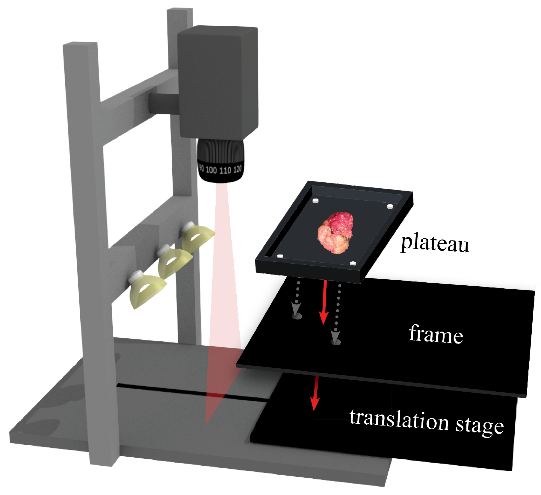
2.1.1. Imaging Setup

Hyperspectral data were acquired with two push-broom hyperspectral imaging systems (Specim, Spectral Imaging Ltd., Oulu, Finland) that operate in the visual (400–1000 nm) and near-infrared (900–1700 nm) wavelength range. The edges of the spectral range of both cameras exhibit a low sensitivity and were removed. The remaining spectral range is 450–951 nm (318 wavelength bands) for the VIS camera and 954–1650 nm (210 wavelength bands) for the NIR camera. In addition, the sensor’s spatial resolution is 0.16 mm/pixel and 0.5 mm/pixel for the VIS and NIR camera, respectively. The scanning speed for both cameras was adjusted to match the cameras spatial resolution of the imaged line. Other technical details of these systems can be found in reference [15]. Figure 1 shows the imaging setup.

2.1.2. Data Preprocessing: Calibration to Diffuse Reflectance

Hyperspectral data analysis and tissue classification were performed using MATLAB 2018b (The MathWorks Inc., Natick, MA, USA). Prior to data analysis, raw hyperspectral data of the tissue sample was calibrated as described in reference [15]. In short, the captured photons counts were converted to diffuse reflectance relative to Spectralon (SRT-99-100, Labsphere Inc., Northern Sutton, NH, USA), which is known to diffusely reflect light with approximately 99%.

2.1.3. Data Preprocessing: Match Hyperspectral Data Obtained with Both Cameras

The sensors’ resolution and the used scanning speed of the two hyperspectral cameras differ. To account for this, the hyperspectral images of both cameras were spatially matched prior to data analysis. For automatic matching, the specimen was placed on a house-made plateau, which was pinned on a frame that fits the translation stage of both cameras (Figure 1) and ensures a reproducible location of each measurement. The plateau and the frame were made of polyoxymethylene that highly absorbs light from 400 to 1700 nm. At the corner edges of the plateau, four circular-shaped white markers were placed that diffusely reflect light with a much higher intensity than the plateau and the tissue, making them easy to segment from the rest of the image. We used these markers and an affine transformation to automatically resize and match the higher-resolution images obtained with the VIS camera to the lower-resolution images obtained with the NIR camera. As a result, we obtain a spectrum with 528 wavelength bands of each pixel in the final hyperspectral image.

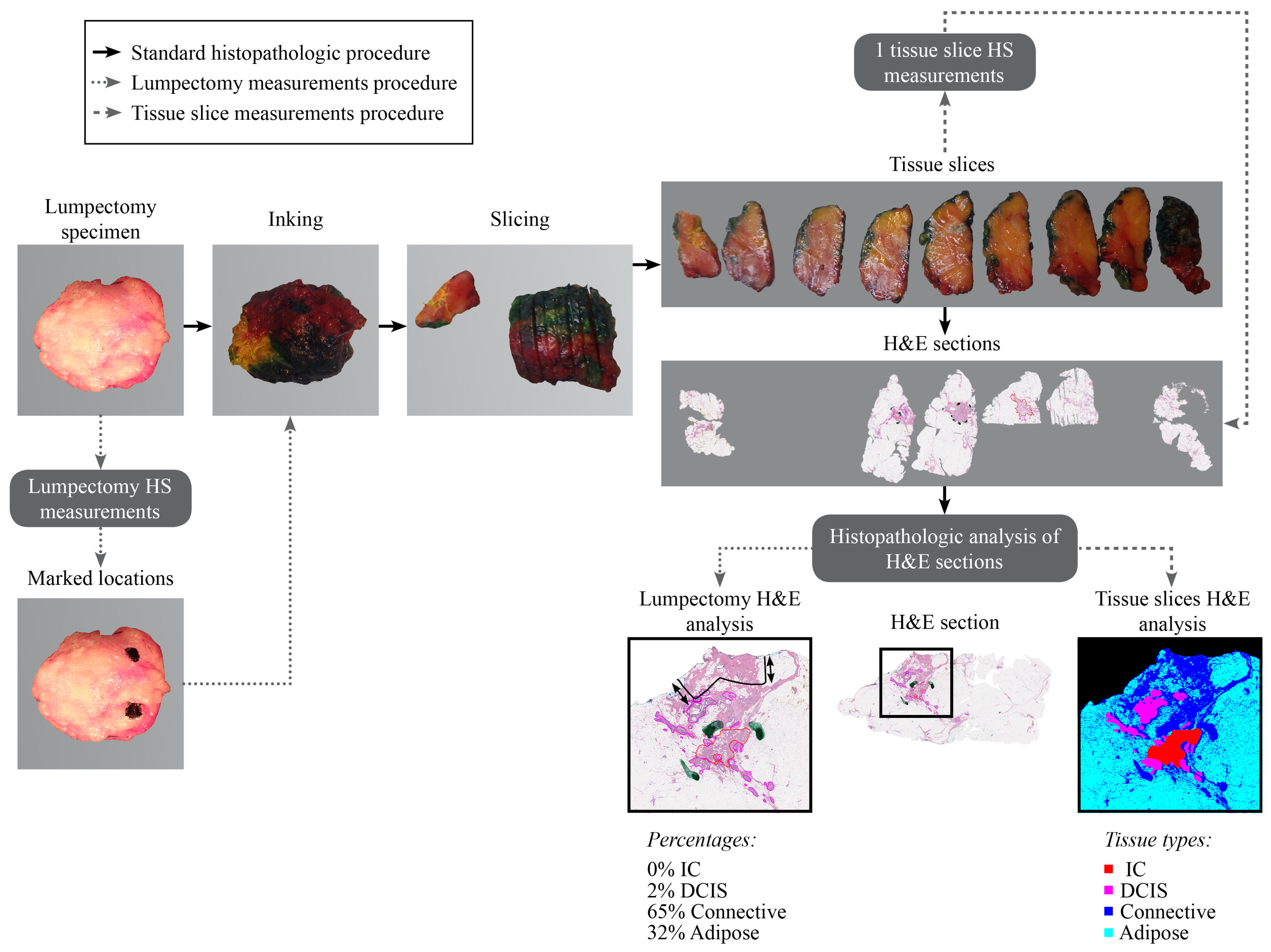
2.2. Data Acquisition and Histopathology Correlation

All measurements were performed on fresh ex vivo tissue from patients receiving primary breast-conserving surgery at the Antoni van Leeuwenhoek hospital. During a standard procedure, the resected specimen was brought to the pathology department where it was inked and gross-sectioned in tissue slices (Figure 2). In this study, we used two datasets: the tissue slices dataset and the lumpectomy dataset. For the tissue slices dataset, we measured tissue slices after inking and gross-sectioning of the resection specimen, while for the lumpectomy dataset, measurements were performed on the specimen immediately after resection. From each patient, either one tissue slice or the unsliced lumpectomy specimen was measured. The major differences in data acquisition and histopathology correlation between the tissue slices and lumpectomy specimen are reported in

Table 1. Differences in data acquisition and histopathology correlation between tissue slices and lumpectomy specimens.

	Tissue Slices Dataset	Lumpectomy Dataset
Data acquisition
Inclusion	Mastectomy and lumpectomy specimen	Lumpectomy specimen
Time in clinical workflow	After inking and slicing the specimen	Directly after resection
Measured surface
cut with	Metal knife (at the pathology department)	Ablation knife (during surgery)
flatness	As flat as possible	Spherical shaped
Histopathology	H & E section parallel	H & E section perpendicular
	to measured side	to measured surface
Spatial correlation	High	Low
Depth information	Low	High

. This study was performed in compliance with the Declaration of Helsinki and approved by the Institutional Review Board of The Netherlands Cancer Institute/Antoni van Leeuwenhoek (Amsterdam, The Netherlands). According to Dutch law (WMO), no written informed consent from patients was required.

2.2.1. Tissue Slices Dataset

In total, 42 tissue slices from different patients were measured using hyperspectral imaging setup. The procedure for data acquisition and histopathology correlation of the tissue slices was described in detail in references [15,16,17,18]. In short, we selected one tissue slice in consultation with the pathologist, containing both healthy and tumor tissue, which we placed on a black rubber surface and imaged with both hyperspectral cameras. After the optical measurements, the measured surface of the tissue slice was processed in hematoxylin and eosin (H & E) stained sections and analyzed by a pathologist. Therefore, the whole measured surface of the tissue slice was annotated with four tissue classes: invasive carcinoma (IC), its potential precursor ductal carcinoma in situ (DCIS), connective tissue (including healthy glandular ducts), and adipose tissue. A distinction was made between all spectra with a tissue class annotation (‘mixed’ dataset) and spectra that only represent the optical properties of a single tissue type (‘pure’ dataset). The ‘pure’ spectra were obtained after removing spectra from the edges (1 mm distance) of each tissue class area in the annotated image. In the remainder of this paper, we will only use the ‘pure’ spectra of the tissue slices dataset.

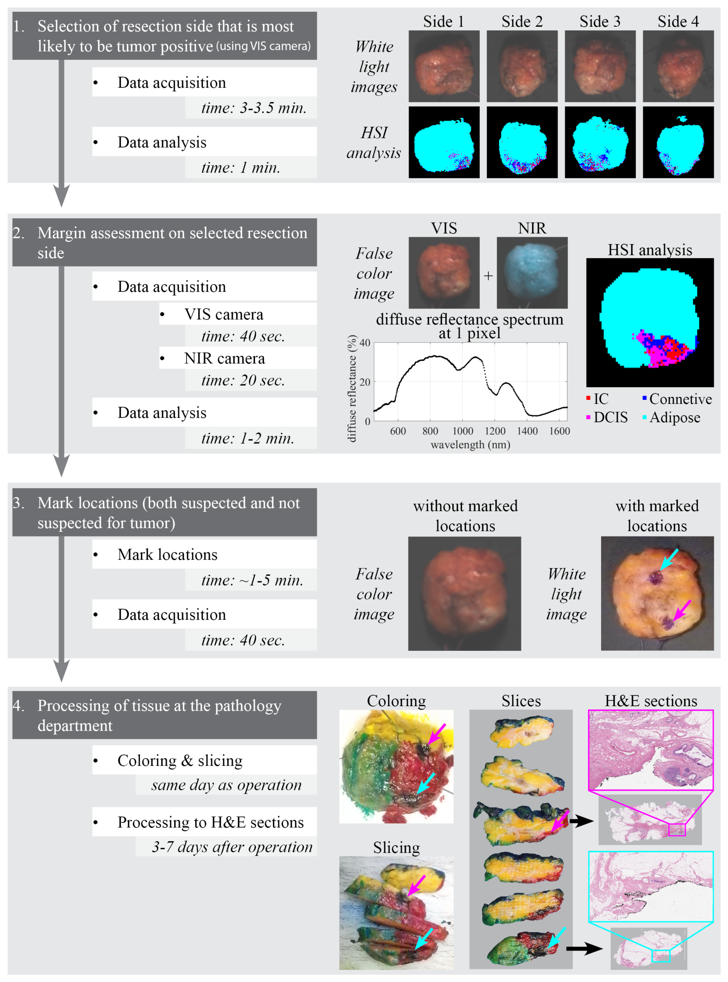
2.2.2. Lumpectomy Dataset

The hyperspectral images of 52 lumpectomy specimens from different patients were included in the lumpectomy dataset. A flowchart of the data acquisition of the lumpectomy dataset is shown in Figure 3. The lumpectomy specimen was considered to be a cube and the entire resection surface was divided into six resection sides. Our aim was to obtain a high correlation of the optical measurements with histopathology. Because this is difficult to achieve when imaging the entire resection surface, only one side was selected for the final analysis instead of the entire resection surface. Of the six resection sides, the nipple and peripheral sides were excluded as H & E sections will be taken parallel to the resection surface and will not provide histopathological information on the margin width [17]. To restrict the time required for all optical measurements, the remaining four sides were first imaged with the VIS camera alone and analyzed with the linear discriminant analysis (LDA) classification algorithm developed on tissue slices in our previous study [15]. With this analysis, the resection side was selected that was most likely to contain a tumor-positive margin. Second, this side was imaged with both cameras. Third, on this selected side, up to four locations were marked with black histopathology ink, which remains visible on the H & E sections under the microscope. To increase the chance of marking tumor positive locations, hyperspectral data were classified with an LDA classification algorithm developed on tissue slices (described in reference [15] and Section 2.2.2 and locations were marked on the specimen that were suspected to (1) be tumor positive (IC and/or DCIS), (2) contain connective tissue, or (3) be adipose tissue. Finally, the lump was scanned again with the VIS camera to retrieve the marked locations and the corresponding spectra on the hyperspectral image of the unmarked lump. All optical measurements, as well as selecting the resection side and marking locations, were performed within 25 min after resection. Afterward, the specimen was transferred to the histopathology department and inked according to standard procedure using blue, yellow, red and green ink. Care was taken not to paint over the black ink. The specimen was sliced, and the marked location(s) were indicated on an overview photo of the tissue slices.

In 3–7 days after surgery, the tissue slices were further processed to H & E sections and digitized using Aperio^® ScanScope AT2 (Leica Biosystems, Wetzlar, Germany). The tissue up to 1 mm underneath the black marked locations on the resection margin was analyzed to obtain the percentage of IC, DCIS, connective tissue and adipose tissue underneath the marked locations. To annotate IC and DCIS on the H & E sections, we used delineations drawn by the pathologist. The remaining tissue was annotated as connective or adipose tissue by thresholding all RGB channels of the H & E section at 90%: Connective tissue colors pink, and adipose tissue is washed away and therefore shows up white on the H & E image.

In addition to obtaining the percentage of tissue in the H & E section, a location was labeled tumor-positive or tumor-negative. Since all measurements were performed in the Antoni van Leeuwenhoek hospital, the Dutch guidelines for resection margin assessment were used in this study. According to this guideline [19], a resection margin is tumor positive if malignant cells are found on the inked resection margin. In the case of DCIS, this would lead to a re-operation. In the case of IC, a re-operation is required only if more than 4 mm of the resection surface is affected. We aim to use hyperspectral imaging to reduce the number of patients that require a re-operation. Therefore, in this study, we focus on detecting the tumor positive margins that lead to a re-operation.

2.3. Hyperspectral Data Analysis

As shown in

Table 2. Data description of tissue slices and lumpectomy specimens.

	Tissue Slices Dataset	Lumpectomy Specimen Dataset
Patient and specimen characteristics
Number of patient	42	52
Patient age (mean ± std)	55.8 ± 10.9	57.7 ± 10.4
Patient ACR (mean ± std)	2.81 ± 0.74	2.46 ± 0.80
Specimen size (mean range)	surface: 15 cm${}^2$ (4–26)	volume: 51 cm${}^3$ (6–240)
	thickness: 4.6 mm (2.5–8)	minimum thickness: 10 mm
Specimens surface flatness	As flat as possible	Spherical shaped
Obtained data
Tissue type measurements ${}^{†}$	spectra/# patients	locations/# patients
Invasive carcinoma	6054/20	5/5
Ductal carcinoma in situ	320/8	3/3
Connective	1180/15	44 ${}^{‡}$/33
Adipose	60,622/42	58 ${}^{‡}$/46
Purity measurement	‘pure’ and ‘mixed’ data	‘mixed’ data
Margin assessment	No	Yes

${}^{†}$ Tissue type according to histopathologic assessment of the corresponding H & E sections. For the lumpectomy specimens, the tissue type of the H & E section is (1) the tissue type most present within 1 mm of the black-colored resection surface or (2) IC/DCIS if present. ${}^{‡}$ Three of these measurements contained exact 50% connective and 50% adipose tissue. In this table, they were added to the number of tissue type measurements of connective tissue.

, there are differences between the tissue slices dataset and the lumpectomy dataset. In Section 2.3.1, we discuss the difference in the measured surface between the two datasets. In Section 2.3.2, we discuss the difference in sample thickness and the possible effect on the measured diffuse reflectance spectra. In Section 2.3.3, the machine learning approach is described that is used to classify hyperspectral data.

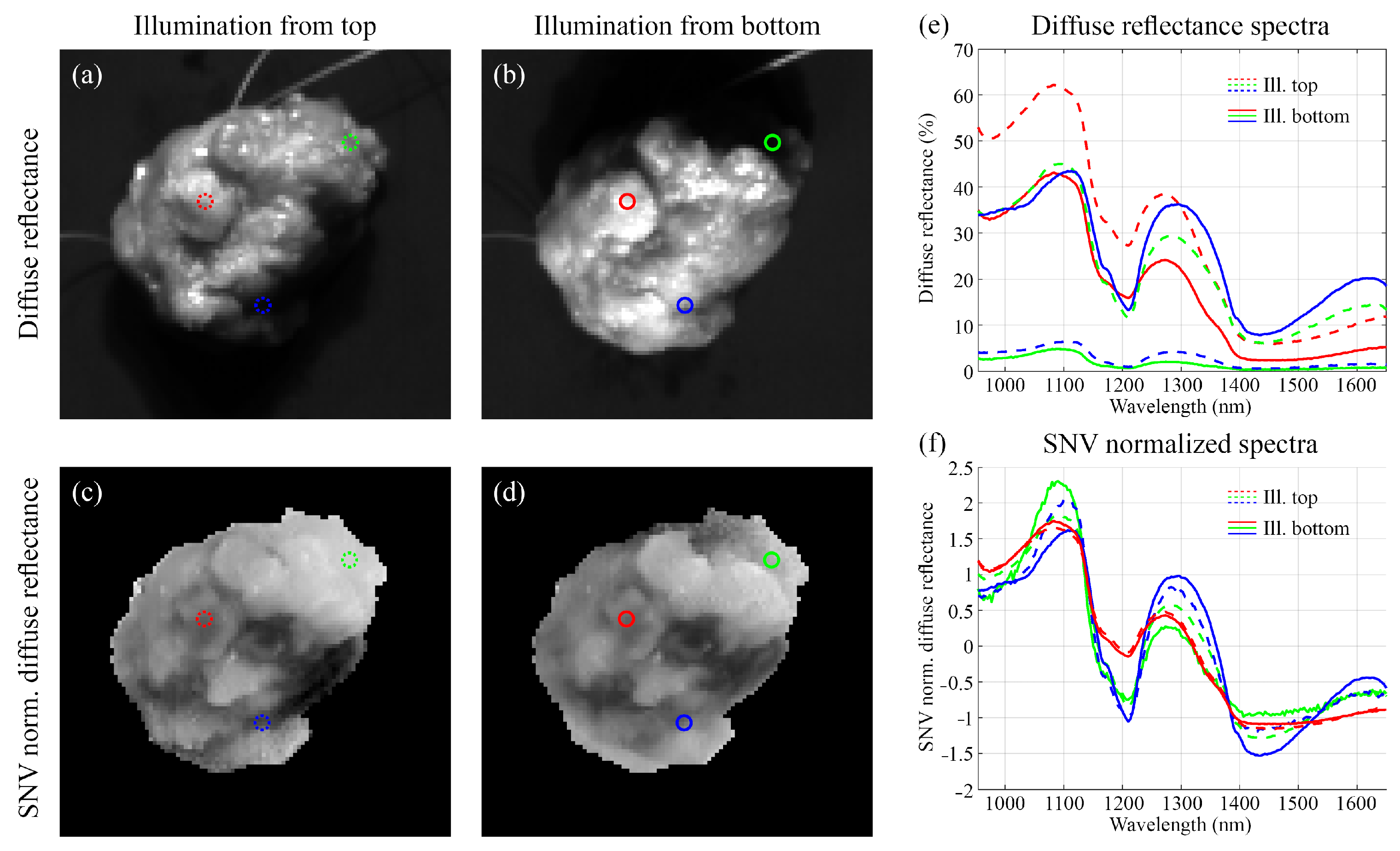
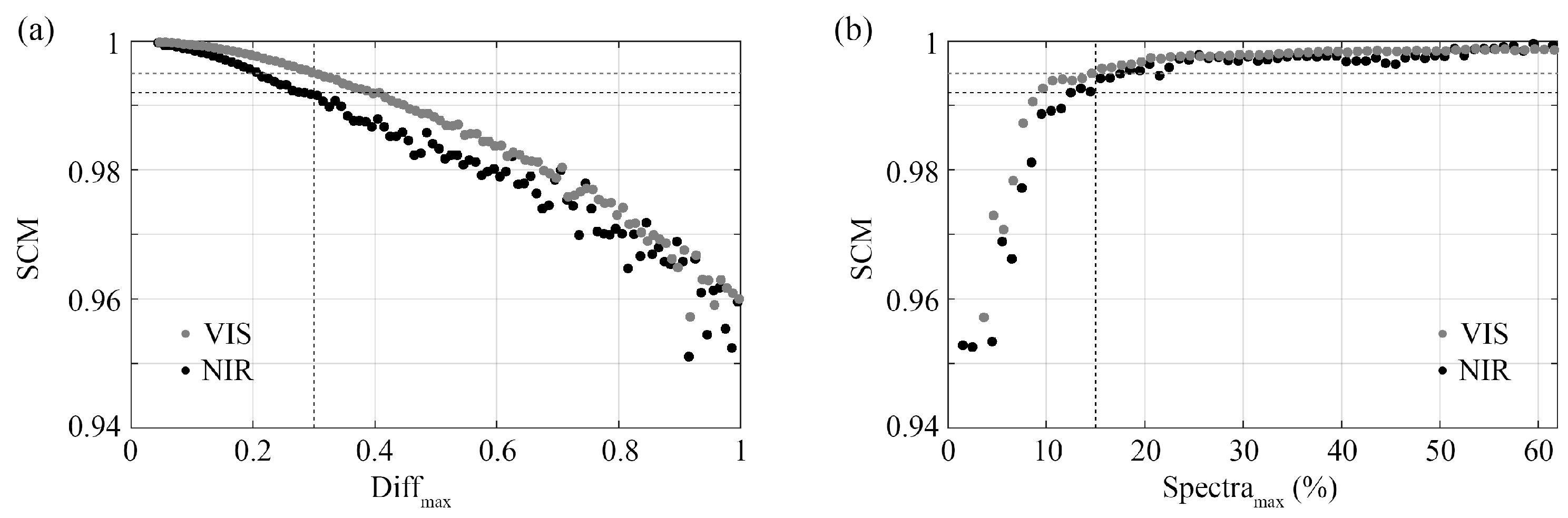
2.3.1. Characteristics of the Measured Surface

Due to the oblique illumination in our measurement setup, the flatness of the tissue has an influence on the measured spectrum that is not related to the optical properties within the tissue. For the tissue slices, we showed that Standard Normal Variate (SNV) normalization can correct for these differences [15]. With SNV each individual spectrum is normalized to a mean of zero and a standard deviation of one [20]. However, because the slices are as flat as possible and the lumpectomy surface is spherically shaped, we need to determine if SNV can also correct for these differences in the spherically shaped lumpectomy samples. To do so, a lumpectomy specimen was measured twice and rotated ${180}^{°}$ so that the tissue was illuminated from a different point of view. By matching these two images, the spectra of individual pixels could be compared. The SNV normalized diffuse reflectance spectra were compared using the spectral correlation measure (SCM) [21], which considers both brightness differences and shape differences between spectra. The SCM is given as

$$SCM\left(s_i{s}_j\right) = \frac{n{\sum }_1^n{s}_i{s}_j-{\sum }_1^n{s}_i{\sum }_1^n{s}_j}{\sqrt{\left(n{\sum }_1^n{s}_i^2-{\left({\sum }_1^n{s}_i\right)}^2\right)\left(n{\sum }_1^n{s}_j^2-{\left({\sum }_1^n{s}_j\right)}^2\right)}},$$

(1)

where $SCM\left(s_i{s}_j\right)$ is the SCM of the SNV normalized spectra obtained before ($s_i$) and after ($s_j$) the specimen was rotated ${180}^{°}$. n is the number of wavelengths. An SCM of 0 and 1 represent no correlation and the highest correlation between spectra, respectively.

2.3.2. Influence of Tissue Thickness Underneath the Measured Surface on Measured Spectrum

The penetration depth of light varies with tissue composition and wavelength [10,14,22,23]. In tissue with a thickness less than the penetration depth, some of the wavelengths can penetrate through the tissue and be absorbed by the rubber or polymethylene underneath the tissue. Therefore, less light will be diffusely reflected and collected by the camera. Since the thickness of the slices is less than the lumpectomy specimens, we expect spectral differences at wavelengths that penetrate the tissue deeper than the minimum tissue slice thickness. To accurately compare spectra from the tissue slices dataset and the lumpectomy dataset, these wavelengths should be excluded from the analysis.

To estimate the penetration depth, we used the optical properties from the lumpectomy measurements, which we estimated using an analytical fit model based on diffusion theory, given as [24]:

$$R_d = \frac{{\alpha }^{\prime }}{1+2k(1-{\alpha }^{\prime })+(1+\frac{2k}{3})\sqrt{3(1-{\alpha }^{\prime })}},$$

(2)

where ${\alpha }^{\prime } = \frac{{\mu }_s^{\prime }}{{\mu }_s^{\prime }+{\mu }_a}$ and $k = \frac{1+r_d}{1-r_d}$. $r_d$ is the internal reflection coefficient for diffuse light and depends on the refractive index of the sample, which was set to be 1.33. ${\mu }_s^{\prime }$ and ${\mu }_a$ are, respectively, the scattering and absorption coefficients and here represented as [25]:

$${\mu }_s^{\prime } = {\mu }_{s,800}^{\prime }\left(f_{mie}{\left(\frac{\lambda }{800\mathrm{nm}}\right)}^{-b}+(1-f_{mie}){\left(\frac{\lambda }{800\mathrm{nm}}\right)}^{-4}\right),$$

(3)

$${\mu }_a = C.v_{blood}.{\mu }_{a,blood} + v_{WL}\left(\left(1-\left(\frac{\left[lipid\right]}{\left[lipid\right]+\left[water\right]}\right)\right).{\mu }_{a,water}\left(\lambda \right) + \left(\frac{\left[lipid\right]}{\left[lipid\right]+\left[water\right]}\right).{\mu }_{a,lipid}\left(\lambda \right)\right),$$

(4)

with

$${\mu }_{a,blood} = (1-St{O}_2){\mu }_{a,Hb}\left(\lambda \right) + St{O}_2{\mu }_{a,Hb{O}_2}\left(\lambda \right),$$

(5)

$$C\left(\lambda \right) = \frac{1-exp(-R.{\mu }_{a,blood})}{R.{\mu }_{a,blod}},$$

(6)

where ${\mu }_{s,800}^{\prime }$ is the reduced scattering at 800 nm, b the scatter power and $f_{mie}$ the fraction Mie scattering with respect to Rayleigh scattering. ${\mu }_{a,water}$ and ${\mu }_{a,lipid}$ are the absorption coefficients of water and lipid, respectively, and $\left[lipid\right]$ and $\left[water\right]$ correspond to the concentration of lipid and water, respectively. $v_{WL}$ is the fraction of water and lipid in the tissue and assumed to be 100% in the near-infrared wavelength region and nearly 0% in the visual wavelength range. $v_{blood}$ and $St{O}_2$ correspond to the blood volume fraction and the level of hemoglobin saturation by oxygen, respectively. ${\mu }_{a,Hb}$ and ${\mu }_{a,Hb{O}_2}$ are the absorption coefficients of hemoglobin and oxyhemoglobin, respectively, and R corresponds to the effective vessel diameter. The measured spectra were fitted using a nonlinear least-squares inversion algorithm, and for each estimated value, a 95% confidence interval was computed that was used to assess the reliability for each fit parameter.

By applying the analytical fit model to the measured spectra on the lumpectomy specimens, we obtained the absorption and scattering coefficients that can be used to estimate the penetration depth, which is given by:

$$d_{eff} = \frac{1}{\sqrt{3{\mu }_a({\mu }_a+{\mu }_s^{\prime })}},$$

(7)

The minimum thickness of the tissue slices is 2.5 mm [15]. Therefore, by excluding wavelengths with a penetration depth above 2.5 mm, the spectra obtained on the tissue slices should be comparable with the spectra obtained on the lumpectomy specimens.

2.3.3. Tissue Classification Using a Machine Learning Approach

Using LDA and the full wavelength range of both hyperspectral cameras, previous research of our group showed that IC, DCIS, connective and adipose tissue in tissue slices can be classified as tumor or healthy tissue in 99%, 95%, 95%, and 100%, respectively, [15]. However, we expect that some wavelengths in the range of 450–1650 nm will have a penetration depth above 2.5 mm. As such, a new LDA algorithm will be developed using only the wavelengths with a penetration depth up to 2.5 mm. To allow for an accurate comparison between these two algorithms, the same training and test sets from the tissue slices dataset were used. Subsequently, the new algorithm will be applied to the lumpectomy dataset.

3. Results

3.1. Data Description

Table 2 shows the patient and specimen characteristics in the slices and lumpectomy dataset. Both patient groups have a similar age. The American College of Radiology (ACR) score, which reflects the breast density (1 = lowest density, 4 = highest density), is higher in the slices dataset. The obtained data varies between the two datasets. First, the slices dataset contains more measurements because spectra were obtained from the entire slice whereas for the lumpectomy dataset up to four locations, reflecting multiple spectra, were marked. Second, a limited number of IC and DCIS was measured in the lumpectomy dataset because of the limited number of tumor-positive resection margins. Third, in the tissue slices dataset, we could make a distinction between ‘pure’ and ‘mixed’ data based on the histopathological information obtained afterward as described in Section 2.2.1. For the lumpectomy dataset, this was not possible as locations were marked immediately after the measurements without any information on the spatial distribution of the tissue types on the surface.

From the 52 patients, we measured, 11 patients required an extra operation after the initial procedure, and in two patients, the excised lump contained a positive margin but some extra tissue was excised during the initial operation, which prevented the need for an extra operation. In these 13 patients, the tumor-positive areas were marked with black pathology ink in four patients. In eight out of the nine other patients, the location of the positive margin was at the peripheral or nipple side, which we did not measure with the hyperspectral camera as explained in Section 2.2.2. Therefore, with the presented hyperspectral data acquisition method, we were able to image and mark the tumor positive margin in 4 out of 5 patients that required an extra operation according to the Dutch guidelines. The H & E sections of these four locations and an overview of the histopathological information corresponding to all 110 measured locations are shown in Figure 4. Most locations were measured on connective and adipose tissue and none of the malignant locations contained more than 80% malignant tissue.

3.2. Characteristics of the Measured Surface

The flatness of the surface has an influence on the measured spectrum, as explained in Section 2.3.1. For the relatively flat tissue slices, SNV normalization can correct these differences [15]. For the spherically shaped lumpectomy surface, SNV normalization proved to be a sufficient method as well in areas of sufficient illumination (red spectra in Figure 5f). Where large differences between Figure 5a,b are observed, these are minimized after applying SNV normalization (Figure 5c,d). However, in areas of shadow (blue and green spectra in Figure 5f), the low illumination resulted in a diffuse reflectance spectrum with a low intensity that could not be corrected for by SNV normalization. We determined the minimum intensity a diffuse reflectance spectrum should have in order to be able to use SNV for normalization. Tissue spectra in Figure 5c were subtracted from tissue spectra from Figure 5d and their maximum absolute difference was plotted against the SCM in Figure 6a. We allow a maximum absolute difference of 0.3, which corresponds to an SCM of 0.995 and 0.992 for NIR and VIS, respectively. Therefore, as shown in Figure 6b, the maximum value of the diffuse reflectance should be at least above 15% (with Spectralon as a reference) for the spectra to be reliable after SNV normalization. Spectra that did not fulfill this criterion (for example the blue and green spectra in Figure 5f) were excluded from further analysis.

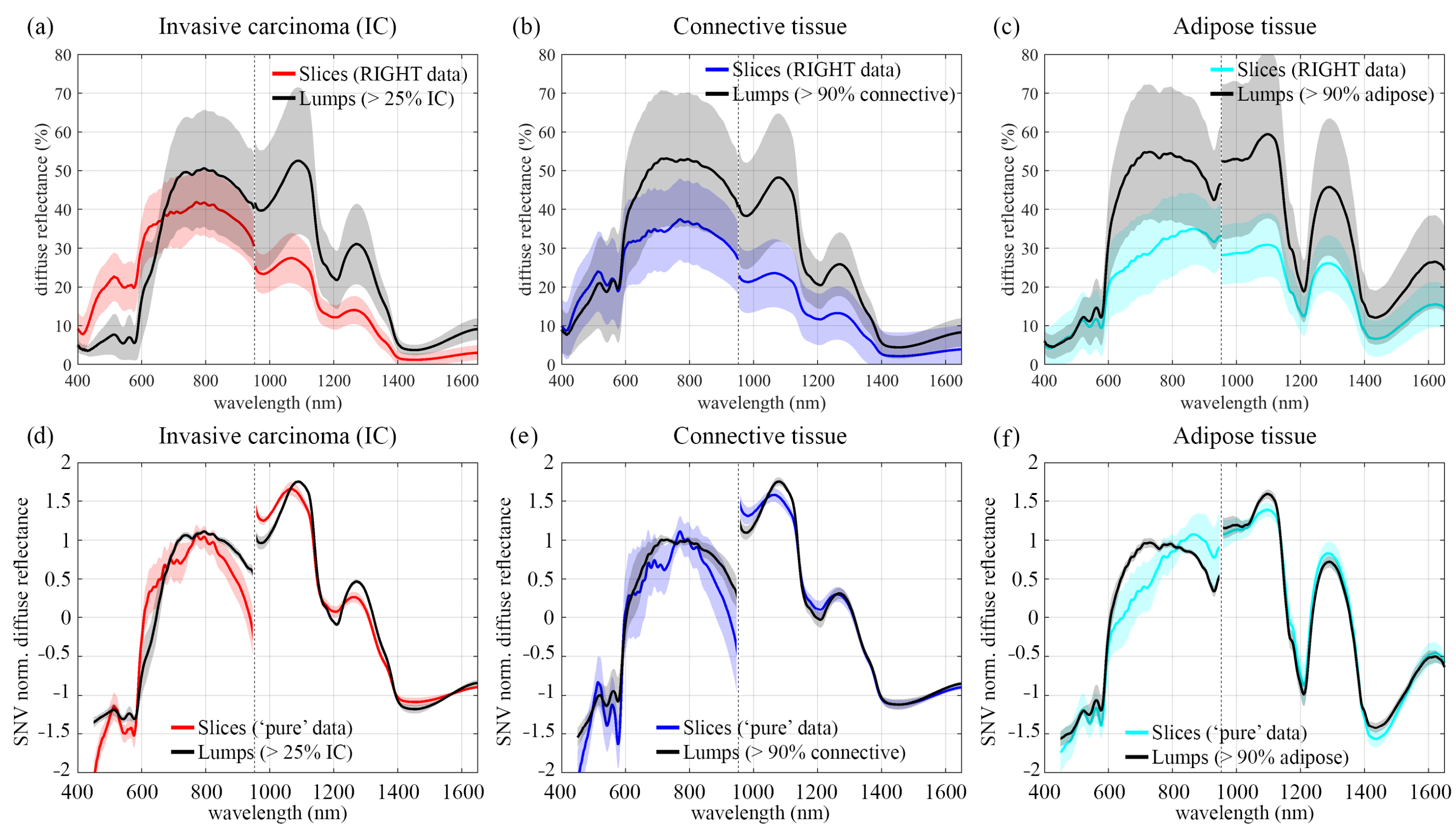
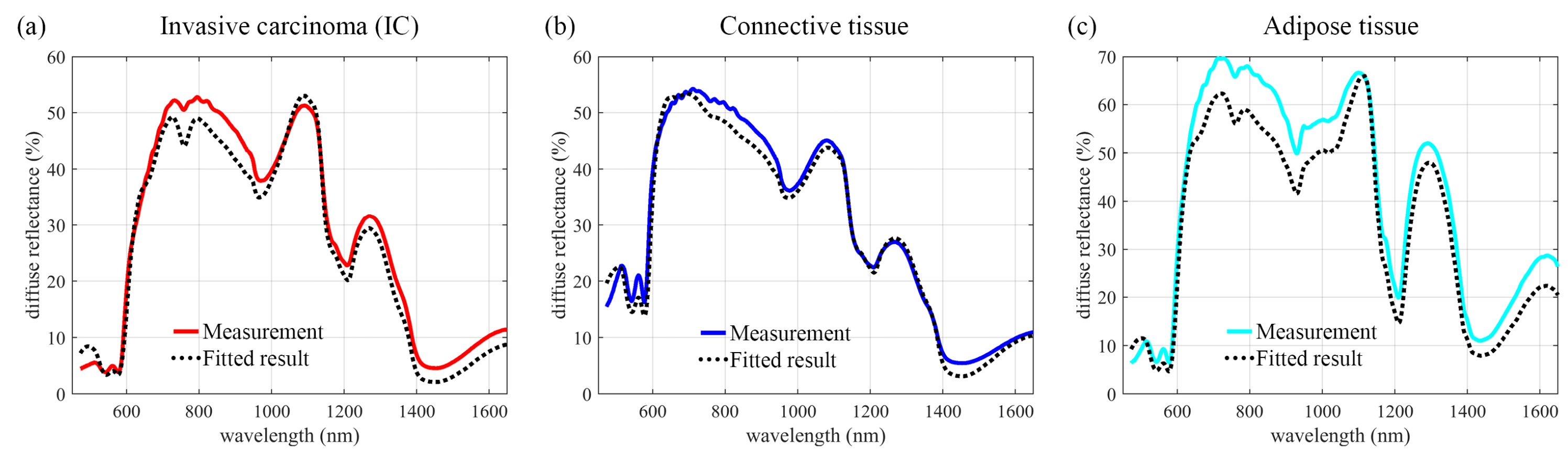
3.3. Influence of Tissue Thickness Underneath the Measured Surface on Measured Spectrum

Spectra in the tissue slices dataset and lumpectomy dataset are compared per tissue type before and after correction for differences in tissue thickness. In this section, only a specific number of spectra from both datasets were used to make an accurate comparison. For the tissue slices dataset, only ‘pure’ spectra were selected (as explained in Section 2.2.1). For the lumpectomy dataset, it was not possible to select ‘pure’ spectra. Therefore, only healthy measurements were selected of which the corresponding H & E section contained more than 90% of the specific tissue type. For IC, including IDC and ILC, measurement locations were selected for which the malignancy measured caused a re-operation. The H & E section of these locations contained 29%, 71% and 79% IC. There was one location, with 6% DCIS in the H & E section, that resulted in a re-operation due to DCIS in the measurement volume. However, due to the low percentage of DCIS in the section, we did not compare this location with spectra from the slices dataset.

3.3.1. Spectral Comparison before Wavelength Reduction

Figure 7 shows the average and standard deviation of the selected spectra in both datasets. The standard deviations around the averaged diffuse reflectance spectra (Figure 7a–c) are large. This is caused by the oblique illumination of our measurement setup and the uneven surface of the tissue. This causes differences in the illumination of the tissue and scatter, nonspecific to the optical properties of the tissue (explained in Section 2.3.1). The spectra obtained with the VIS and NIR cameras are not connected because both cameras have their own suspension system and light sources, causing a slightly different illumination angle. Using SNV normalization as a pre-processing step, the standard deviation around the averaged spectra (Figure 7d–f) is reduced. Since SNV was applied to the spectrum obtained with the VIS and NIR camera individually, the SNV normalized spectra are not connected. In the remainder of this paper, we will only use the SNV normalized spectra for further analysis.

For all tissue types, large differences are observed between the slices data and the lumpectomy data. The largest differences are present in the VIS wavelength range and in between 1000 and 1150 nm in the NIR wavelength range. These differences might be related to the fact that the optical penetration depth in this wavelength region exceeds the thickness of the tissue slices. In one location (Figure 7a, 79% IC), the effects of cutting by cauterization were clearly visible in the H & E section. In comparison with the two other malignant locations, this correlated with a decrease in the mean spectrum between 600 and 650 nm.

Based on the large spectral differences between the slices and lumpectomy data, we expect that classification algorithms developed on the slices dataset may exhibit a lower performance on the lumpectomy dataset.

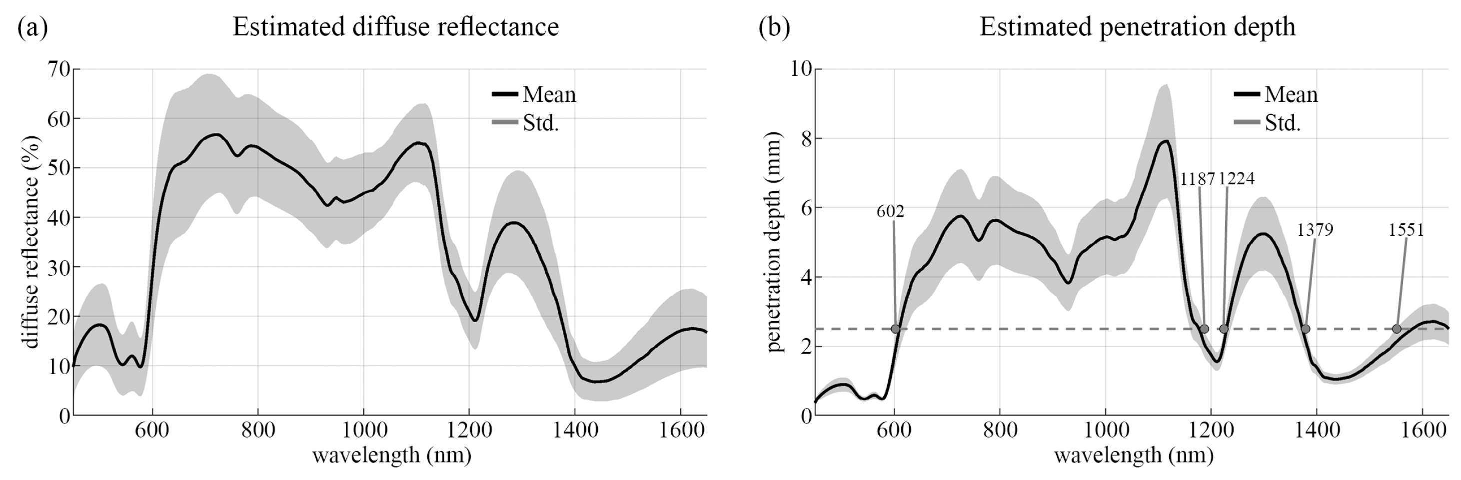
3.3.2. Estimated Penetration Depth

As explained in Section 2.3.2, the penetration depth was estimated using the fitted optical properties of the selected diffuse reflectance spectra in the lumpectomy dataset. An example of a spectral measurement with the corresponding fitted curve is shown in Figure 8 for each tissue type.

Table 3. Estimated fit parameters from lumpectomy measurements (fitted value ± confidence interval).

Tissue Type	Percentage in H & E Section	Scattering			Absorption
		${\mathit{\mu }}_{\mathit{s},800}^{\prime }$	${\mathit{f}}_{\mathit{mie}}$ (%)	${\mathit{b}}_{\mathit{mie}}$	${\mathit{StO}}_2$ (%)	Blood (%)	Fat (%)	H2O (%)
IC	29	2.9 ± 0.9	100 ± 14	0.80 ± 0.76	45 ± 6	8.1 ± 0.7	31 ± 12	69 ± 12
IC	71	6.1 ± 1.2	100 ± 5	0.40 ± 0.37	55 ± 3	6.4 ± 1.0	36 ± 7	64 ± 7
IC	78.5	4.6 ± 1.3	100 ± 9	0.70 ± 0.64	24 ± 6	5.6 ± 1.6	35 ± 11	65 ± 11
Connective	98	24.9 ± 6.9	100 ± 8	0.82 ± 0.78	93 ± 3	2.7 ± 1.0	34 ± 15	66 ± 15
Connective ${}^{†}$	92	25.6 ± 14.8	100 ± 73	2.20 ± 2.33	87 ± 8	4.8 ± 3.6	37 ± 24	63 ± 24
Connective ${}^{†}$	93	5.4 ± 1.2	100 ± 4	0.20 ± 0.55	33 ± 6	3.6 ± 1.2	17 ± 16	83 ± 16
Connective	93	10.1 ± 1.8	100 ± 4	0.50 ± 0.46	75 ± 3	1.5 ± 0.3	43 ± 8	57 ± 8
Connective ${}^{†}$	91	11.0 ± 2.1	100 ± 4	0.35 ± 0.50	70 ± 3	4.6 ± 2.9	5 ± 1	95 ± 1
Adipose	95	15.0 ± 3.0	100 ± 6	0.59 ± 0.53	78 ± 3	4.6 ± 0.9	90 ± 3	10 ± 3
Adipose	96	6.1 ± 1.1	100 ± 6	0.54 ± 0.52	64 ± 4	3.7 ± 0.6	89 ± 2	11 ± 2
Adipose	94	10.2 ± 3.7	100 ± 19	1.34 ± 1.09	78 ± 6	4.4 ± 1.6	91 ± 5	9 ± 5
Adipose	92	10.9 ± 3.8	100 ± 23	1.49 ± 1.19	75 ± 6	6.7 ± 2.4	84 ± 8	16 ± 8
Adipose	92	11.1 ± 2.6	100 ± 10	1.00 ± 0.68	70 ± 4	3.4 ± 0.8	92 ± 2	9 ± 2
Adipose	92	5.7 ± 0.8	100 ± 8	0.45 ± 0.37	73 ± 3	3.2 ± 2.6	91 ± 1	9 ± 1
Adipose ${}^{†}$	92	20.3 ± 13.4	100 ± 70	2.10 ± 2.28	84 ± 10	8.6 ± 5.8	87 ± 10	13 ± 10
Adipose	93	7.2 ± 1.1	100 ± 5	0.54 ± 0.47	71 ± 3	2.6 ± 0.4	92 ± 1	8 ± 1

${}^{†}$ The fitted parameters of this measurement were not included in the estimation of the diffuse reflectance and penetration depth because the confidence interval of $St{O}_2$ was higher than the fitted value.

shows the obtained optical fit parameters for all fitted spectra and their confidence intervals. A combination of fit parameters is expected to be representative for the tissue composition if the measured and fitted curves are similar and the confidence intervals are low. Therefore, fitted parameters of three connective measurements and one adipose measurement were not included in the estimation of the diffuse reflectance and penetration depth because the confidence interval of $b_{mie}$ was higher than the fitted value.

With the obtained optical properties and Equations (2)–(7), we estimated the diffuse reflectance (Figure 9a) and the penetration depth (Figure 9b) in breast tissue. There is a large difference in penetration depth between wavelengths. Especially between 684 and 872 nm, 980–1142 nm, and around 1300 nm, the penetration depth is high with values above 5 mm. At these wavelengths, indeed spectral differences between the tissue slices dataset and lumpectomy dataset (Figure 7) are the largest. This confirms that penetration depth differences cause spectral differences between the two datasets. For an accurate spectral comparison between the slices and lumpectomy dataset, we set the maximum penetration depth that we allow to reach 2.5 mm, which is the minimum thickness of the tissue slices. Thus, the number of wavelengths for further analysis was reduced from 450 to 1650 (528 wavelength bands) to three wavelength ranges: 450–602 nm, 1187–1224 nm, and 1379–1551 nm (total of 164 wavelength bands).

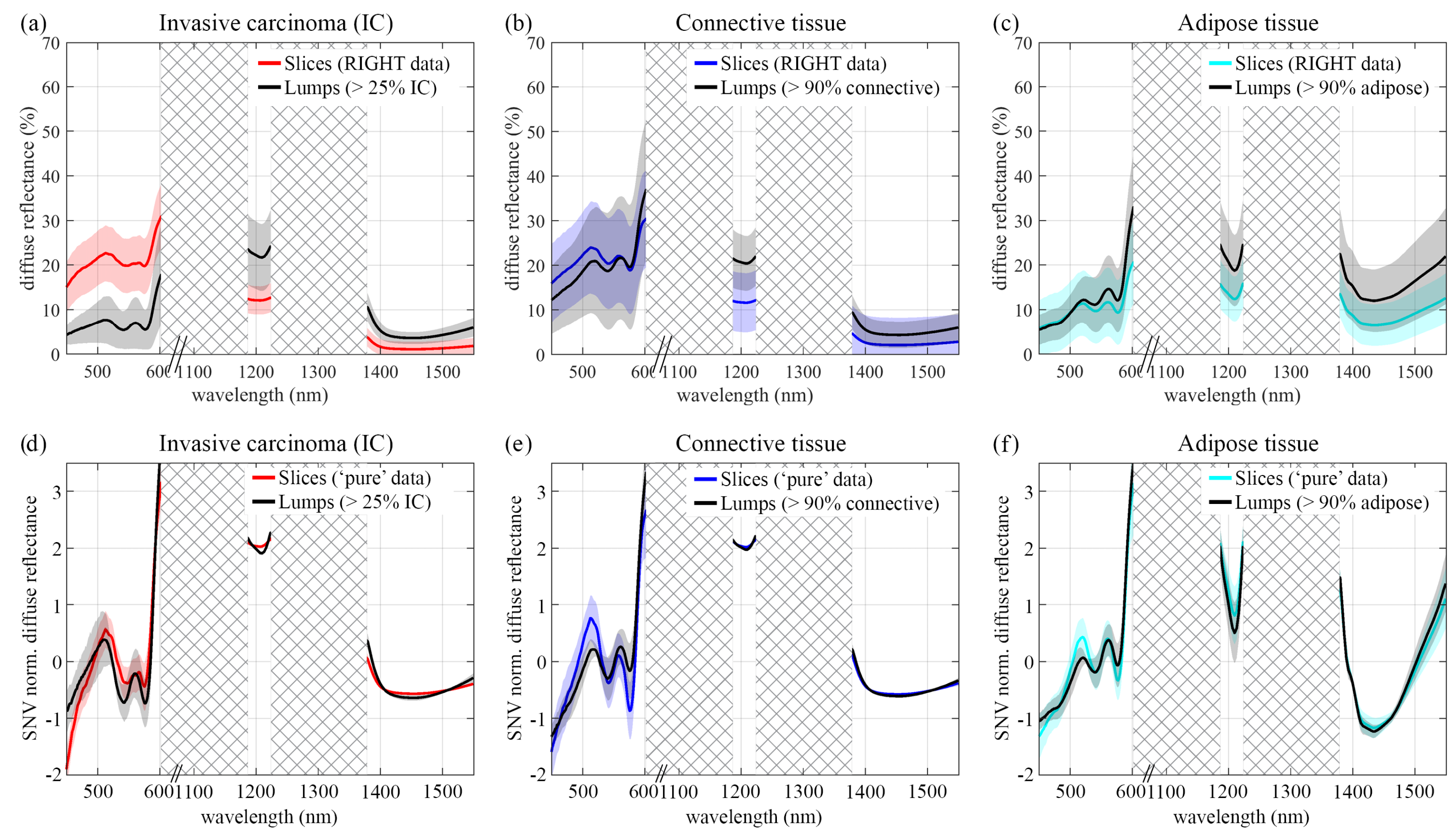
3.3.3. Spectral Comparison after Wavelength Reduction

Figure 10 shows the selected SNV normalized diffuse reflectance spectra after wavelength reduction. In comparison with Figure 7, indeed the spectra are more similar between the tissue slices dataset and the lumpectomy data. In the NIR (>1176 nm), the spectra of the slices and lumps are most similar with an SCM of 1.00, 1.00 and 0.99 for IC, connective and adipose tissue, respectively. The maximum difference between the spectra was 0.31, 0.11 and 0.31. In the VIS (<602 nm), spectra from the slices dataset and the lumpectomy dataset deviate more with an SCM of 0.92, 0.93 and 0.98 for IC, connective and adipose, respectively, and a maximum spectral difference of 1.04, 0.70 and 0.42. In addition, for IC around 1200 nm, the shape of the lumpectomy spectra is steeper which would indicate that these spectra contain more fat. This corresponds with the fat percentage in the H & E sections: 19%, 9%, and 6%.

After wavelength reduction, the spectra of slices and lumpectomy data are more similar (Figure 7 vs. Figure 10). Therefore, in Section 3.4.1, hyperspectral analysis was only performed using wavelengths with a penetration depth up to 2.5 mm.

3.4. Classification Results after Wavelength Reduction Using LDA

3.4.1. Tissue Slices

Table 4. Classification results before and after wavelength reduction: Recall for each tissue type.

		Before Wavelength Reduction [15]	After Wavelength Reduction
	Number of	VIS	VIS + NIR
	Spectra	NIR (450–1650 nm)	(450–602 & 1187–1224 & 1379–1551 nm)
Tumor	3312	99%	79%
IC	3200	99%	80%
DCIS	112	95%	77%
Healthy	21,227	99%	90%
Connective	468	94%	68%
Adipose	20,759	100%	96%

shows the classification results using LDA and the tissue slices dataset before and after wavelength reduction. In a similar approach described in [15], the splitting of the whole dataset into a training set (70% of the images) and a test set (30% of the images) was performed randomly while keeping spectra from one patient together. The recall was the percentage of pixels that were correctly classified as tumor or healthy tissue, using histopathologic assessment as ground truth. The classification results decreased after wavelength reduction: The performance of both tumor and connective tissue detection decreased from values of 99% to 79% and 94% to 68%, respectively. Only the detection of adipose tissue, with values higher than 94%, remained high after wavelength reduction.

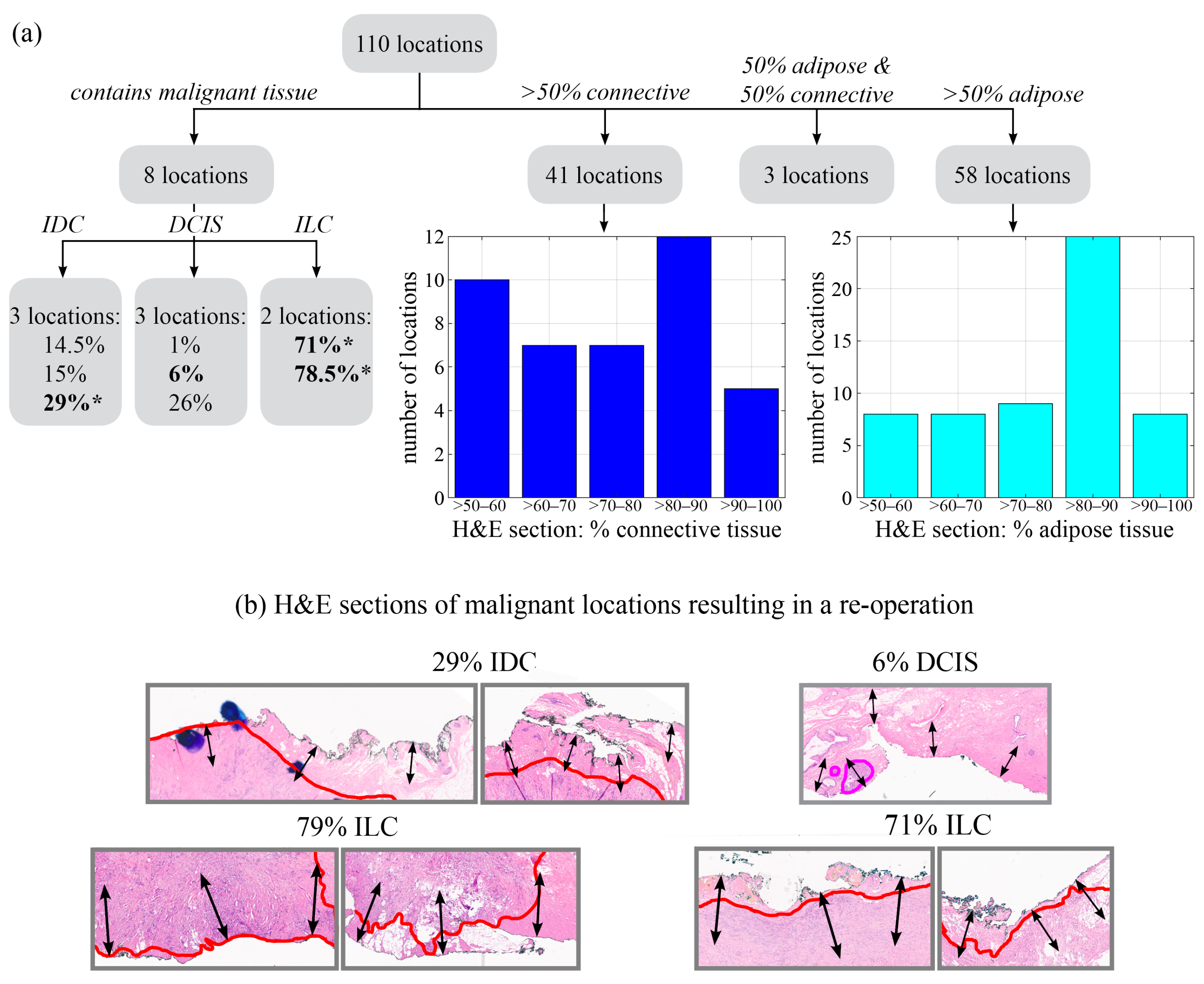
3.4.2. Lumpectomy Specimen

The LDA algorithm after wavelength reduction was applied to all 110 locations in the lumpectomy dataset. As expected from Table 4, the classification results on the lumpectomy dataset were insufficient: Of the four locations that contained malignant tissue and required a re-operation, only one was classified as tumor tissue. Figure 11 shows the classification results of the healthy tissue locations. In these locations, the performance was higher if a measurement was more ‘pure’. False positive tumor classifications occurred only when the fat percentage in the H & E section was lower than 50%.

4. Discussion and Conclusions

When investigating the potential of hyperspectral imaging for intraoperative breast cancer detection, it is challenging to image the actual resection surface to allow for intraoperative feedback while obtaining a high correlation with histopathology. As such, previous research of our group showed the potential of hyperspectral imaging to discriminate tumor from healthy tissue using fresh breast tissue slices [14,15]. By imaging tissue slices, an extensive reliable hyperspectral database was created with a high correlation with histopathology and enough measurements on both healthy and tumorous tissue to develop reliable classification algorithms. In the current study, we imaged the resection surface of lumpectomy specimens and presented a method that allowed us to (1) obtain a high correlation with histopathology and (2) increased the likelihood to measure tumor-positive resection margins. Next, we compared the hyperspectral data obtained on the tissue slices and lumpectomy specimens. Due to the difference in tissue thickness and the penetration depth of light, spectra in both datasets varied. After reducing the number of wavelengths so that only wavelengths with a penetration depth less than 2.5 mm (minimum thickness of tissue slices) remained, the spectral similarity increased. However, with the remaining wavelength, the classification performance on both tissue slices and lumpectomy specimens were insufficient for clinical application. Therefore, even though the tissue slices dataset could be used to investigate the potential of hyperspectral imaging as a margin assessment technique for breast surgery, algorithms developed with the slices data cannot be used directly to classify lumpectomy specimens.

The penetration depth of light varies both with wavelength and tissue composition and was estimated with a model based on diffusion theory. This model assumes an optically homogeneous and infinite medium and extracts optical parameters from a measured diffuse reflectance spectrum. However, in the lumpectomy data that we measured, the breast tissue was inhomogeneous. Therefore, different wavelengths in one diffuse reflectance spectrum reflect different measurement volumes, that can have different optical properties. As the model assumes that the diffuse reflectance spectrum reflects a single set of optical properties, extracting optical properties from a spectrum reflecting multiple optical properties might be prone to errors. This explains why the fitted and measured spectra in Figure 8 did not completely overlap and why, for some parameters, the confidence intervals are relatively high. When the penetration depth is known, a fitting algorithm can be applied on separate wavelength ranges with a uniform measurement volume, reflecting a single set of optical properties [26]. However, in the present work, the penetration depth was unknown. Therefore, we used the fitted optical parameters to obtain an estimation of the penetration depth.

By excluding wavelengths with penetration depth higher than 2.5 mm, spectra of the slices and lumpectomy datasets are more similar (Figure 7 vs. Figure 10). The highest difference between the two datasets and the lowest SCM was observed in the VIS wavelength range. In this wavelength range, spectra are primarily shaped by (de)oxyhemoglobin. The difference between the two datasets can be related to the difference in time after resection when the specimens are measured: Lumpectomy specimens are measured immediately after resection whereas the tissue slices are first inked and sliced. This time delay might have an effect on blood volume fraction and $St{O}_2$ in the tissue as reported by Bydlon et al. [27]. They stated that especially $St{O}_2$ was an unreliable parameter due to excessive changes in oxygenated and deoxygenated hemoglobin post-excision. In their study, the blood volume fraction changed over time, but until 63 minutes after excision, these changes were less than the differences between positive malignant sites and connective or adipose tissue.

Another explanation of the difference between the two datasets may be the difference in cutting the tissue by cauterization, used during surgery, or by using a regular knife, used while slicing the specimen. Bydlon et al. showed that there was a difference in the total blood volume in lumpectomy (cut with cauterization) and mastectomy (cut with a knife) specimens and they assumed that by cauterization of the vasculature, blood is prevented from draining out of the vessels [27]. Spliethoff et al. reported on the effect of thermal coagulation on blood samples and found a change in shape in between 600 and 650 nm that was related to a decrease in oxyhemoglobin related features [28]. A similar effect was observed in this study, as shown in Figure 7a. However, since this wavelength range was excluded after wavelength reduction, this effect of cauterization was expected to be minimal. In a study by Adank et al., the influence of cutting by coagulation on diffuse reflectance spectra in the NIR was small in muscle tissue and nonexistent in adipose tissue [29]. Therefore, we expect a minimum effect in the NIR wavelength region. With the remaining wavelengths, it is possible to discriminate adipose tissue from the other tissue types on the tissue slices dataset, but it was more challenging to distinguish connective tissue from malignant tissue. With the LDA classifier and the limited wavelengths range, the performance for detecting adipose tissue was high (>94%) while the performance for detection of either tumor (56% using VIS), connective tissue (35% using NIR) or both tumor and connective tissue (79% and 68%, respectively, using VIS + NIR) was low. These classification results on the slices dataset may not be good enough for accurate discrimination between tumor and connective tissue in clinical practice. This was confirmed with the lumpectomy dataset: only 1 of 4 malignant locations that required a re-operation were found with LDA.

As explained in the introduction, obtaining a high correlation of hyperspectral measurements on lumpectomy specimens with histopathology is difficult. In addition, it is challenging to find tumor-positive margins on the specimen by eye. With the presented data acquisition method, we were able to obtain a high correlation with histopathology and mark the tumor positive margin in 4 out of 5 patients that required an extra operation. Nevertheless, in the lumpectomy dataset, there were only a limited number of malignant locations in comparison with the number of healthy locations, as the number of specimens with a tumor-positive margin was limited. In addition, none of the malignant locations contained more than 80% IC or DCIS in the corresponding H & E section. Therefore, in contrast to the slices dataset, the lumpectomy dataset contained no ‘pure’ tumor measurements. For example, in the H & E section of location 1 in Figure 4b, there is a rim of adipose tissue between the ILC border and the resection surface. This affects the measured spectrum and will increase the likelihood that this malignant location is classified as adipose tissue.

Because the dataset created on the lumpectomy specimens was not enough to develop reliable classification algorithms, we aimed in this study to develop classification algorithms with the slices dataset and apply these on the lumpectomy specimens for classification. However, this approach proved to be insufficient for obtaining good classification results. The problem of slightly different training and testing datasets is a known problem in the field of machine learning, which can be accounted for by using transfer learning and domain adaptation techniques [30]. Therefore, an algorithm trained on the tissue slices would be re-purposed to classify the lumpectomy data. However, such a technique requires much more lumpectomy data than the data available in this study. In general, to improve the classification results on the lumpectomy specimens, the amount of lumpectomy data, and especially the number of malignant locations, should be increased. This can be achieved, for example, by cutting the resection specimen by cauterization further after performing the standard procedure for breast-conserving surgery. Therefore, the surgeon would increase the number of tumor-positive margins that can be optically measured, without affecting the current clinical workflow and clinical outcome. Obtaining a larger lumpectomy dataset would allow for the use of transfer learning or the training of classification algorithms on lumpectomy data instead of slices data. By doing so, no wavelengths need to be removed to correct for sample thickness differences and the entire spectral range of our cameras, i.e., all wavelengths, can be used for creating algorithms.

In summary, we presented a methodology to obtain a high correlation of hyperspectral measurements on lumpectomy specimen with histopathology and showed that this allowed us to mark 4 out of 5 tumor positive margins that were not visible with the human eye. In addition, we showed that classification algorithms developed on tissue slices could not be used directly on lumpectomy data. After wavelength reduction to limit the sampling depth, adipose tissue could be clearly discriminated from other tissue types but differentiating malignant from connective tissue was more challenging. For improved discrimination between malignant and connective tissue, the amount of lumpectomy data, and especially the number of malignant locations, should be increased so that classification algorithms can be adapted and trained on lumpectomy data.

References

1. Landercasper, J. Variability in Reexcision Following Breast Conservation Surgery. Breast Dis. Year Book Q. 2012, 4, 385–387. [Google Scholar] [CrossRef]
2. Gentilini, O.; Gahir, J. An urgent need to reduce re-operation rates after breast conserving surgery. Gland. Surg. 2012, 1, 159. [Google Scholar] [CrossRef]
3. Jeevan, R.; Cromwell, D.; Trivella, M.; Lawrence, G.; Kearins, O.; Pereira, J.; Sheppard, C.; Caddy, C.; Van Der Meulen, J. Reoperation rates after breast conserving surgery for breast cancer among women in England: Retrospective study of hospital episode statistics. BMJ 2012, 345, e4505. [Google Scholar] [CrossRef] [Green Version]
4. Lagios, M.; Silverstein, M. Implications of New Lumpectomy Margin Guidelines for Breast-Conserving Surgery: Changes in Reexcision Rates and Predicted Rates of Residual Tumor. Breast Dis. Year Book Q. 2016, 4, 295–296. [Google Scholar] [CrossRef]
5. Merrill, A.L.; Tang, R.; Plichta, J.K.; Rai, U.; Coopey, S.B.; McEvoy, M.P.; Hughes, K.S.; Specht, M.C.; Gadd, M.A.; Smith, B.L. Should new “no ink on tumor” lumpectomy margin guidelines be applied to ductal carcinoma in situ (DCIS)? A retrospective review using shaved cavity margins. Ann. Surg. Oncol. 2016, 23, 3453–3458. [Google Scholar] [CrossRef]
6. Stewart, B.W.; Kleihues, P. World Cancer Report; IARC Press: Lyon, France, 2003. [Google Scholar]
7. Havel, L.; Naik, H.; Ramirez, L.; Morrow, M.; Landercasper, J. Impact of the SSO-ASTRO margin guideline on rates of re-excision after lumpectomy for breast cancer: A meta-analysis. Ann. Surg. Oncol. 2019, 26, 1238–1244. [Google Scholar] [CrossRef] [PubMed]
8. Schulman, A.M.; Mirrielees, J.A.; Leverson, G.; Landercasper, J.; Greenberg, C.; Wilke, L.G. Reexcision surgery for breast cancer: An analysis of the American Society of Breast Surgeons (ASBrS) Mastery SM database following the SSO-ASTRO “no ink on tumor” guidelines. Ann. Surg. Oncol. 2017, 24, 52–58. [Google Scholar] [CrossRef]
9. Vos, E.; Gaal, J.; Verhoef, C.; Brouwer, K.; Van Deurzen, C.; Koppert, L. Focally positive margins in breast conserving surgery: Predictors, residual disease, and local recurrence. Eur. J. Surg. Oncol. 2017, 43, 1846–1854. [Google Scholar] [CrossRef]
10. Lu, G.; Fei, B. Medical hyperspectral imaging: A review. J. Biomed. Opt. 2014, 19, 010901. [Google Scholar] [CrossRef] [PubMed]
11. Lu, G.; Little, J.V.; Wang, X.; Zhang, H.; Patel, M.R.; Griffith, C.C.; El-Deiry, M.W.; Chen, A.Y.; Fei, B. Detection of head and neck cancer in surgical specimens using quantitative hyperspectral imaging. Clin. Cancer Res. 2017, 23, 5426–5436. [Google Scholar] [CrossRef] [PubMed] [Green Version]
12. Halicek, M.; Dormer, J.D.; Little, J.V.; Chen, A.Y.; Myers, L.; Sumer, B.D.; Fei, B. Hyperspectral imaging of head and neck squamous cell carcinoma for cancer margin detection in surgical specimens from 102 patients using deep learning. Cancers 2019, 11, 1367. [Google Scholar] [CrossRef] [PubMed] [Green Version]
13. Baltussen, E.J.; Kok, E.N.; de Koning, S.G.B.; Sanders, J.; Aalbers, A.G.; Kok, N.F.; Beets, G.L.; Flohil, C.C.; Bruin, S.C.; Kuhlmann, K.F.; et al. Hyperspectral imaging for tissue classification, a way toward smart laparoscopic colorectal surgery. J. Biomed. Opt. 2019, 24, 016002. [Google Scholar] [CrossRef] [PubMed]
14. Kho, E.; de Boer, L.L.; Post, A.L.; Van de Vijver, K.K.; Jóźwiak, K.; Sterenborg, H.J.; Ruers, T.J. Imaging depth variations in hyperspectral imaging: Development of a method to detect tumor up to the required tumor-free margin width. J. Biophotonics 2019, 12, e201900086. [Google Scholar] [CrossRef] [PubMed]
15. Kho, E.; Dashtbozorg, B.; De Boer, L.L.; Van de Vijver, K.K.; Sterenborg, H.J.; Ruers, T.J. Broadband hyperspectral imaging for breast tumor detection using spectral and spatial information. Biomed. Opt. Express 2019, 10, 4496–4515. [Google Scholar] [CrossRef] [PubMed] [Green Version]
16. Fabelo, H.; Halicek, M.; Ortega, S.; Szolna, A.; Morera, J.; Sarmiento, R.; Callico, G.M.; Fei, B. Surgical aid visualization system for glioblastoma tumor identification based on deep learning and in vivo hyperspectral images of human patients. In Medical Imaging 2019: Image-Guided Procedures, Robotic Interventions, and Modeling; International Society for Optics and Photonics: Washington, DC, USA, 2019; Volume 10951, p. 1095110. [Google Scholar] [CrossRef]
17. Kho, E.; de Boer, L.L.; Van de Vijver, K.K.; van Duijnhoven, F.; Peeters, M.J.T.V.; Sterenborg, H.J.; Ruers, T.J. Hyperspectral imaging for resection margin assessment during cancer surgery. Clin. Cancer Res. 2019, 25, 3572–3580. [Google Scholar] [CrossRef] [PubMed] [Green Version]
18. de Boer, L.L.; Kho, E.; Nijkamp, J.; Van de Vijver, K.K.; Sterenborg, H.J.; ter Beek, L.C.; Ruers, T.J. Method for coregistration of optical measurements of breast tissue with histopathology: The importance of accounting for tissue deformations. J. Biomed. Opt. 2019, 24, 075002. [Google Scholar] [CrossRef]
19. Nederland, I.K. Landelijke Richtlijn Mammacarcinoom Versie 2.0 (Dutch Guideline Breast Cancer Version 2.0). 2016. Available online: https://www.oncoline.nl/uploaded/docs/mammacarcinoom/Dutch%20Breast%20Cancer%20Guideline%202012.pdf (accessed on 23 August 2021).
20. Barnes, R.; Dhanoa, M.S.; Lister, S.J. Standard normal variate transformation and de-trending of near-infrared diffuse reflectance spectra. Appl. Spectrosc. 1989, 43, 772–777. [Google Scholar] [CrossRef]
21. Van der Meer, F. The effectiveness of spectral similarity measures for the analysis of hyperspectral imagery. Int. J. Appl. Earth Obs. Geoinf. 2006, 8, 3–17. [Google Scholar] [CrossRef]
22. Randeberg, L.L.; Larsen, E.L.; Svaasand, L.O. Hyperspectral imaging of blood perfusion and chromophore distribution in skin. In Photonic Therapeutics and Diagnostics V; International Society for Optics and Photonics: Washington, DC, USA, 2009; Volume 7161, p. 71610C. [Google Scholar] [CrossRef]
23. Zhang, H.; Salo, D.C.; Kim, D.M.; Komarov, S.; Tai, Y.C.; Berezin, M.Y. Penetration depth of photons in biological tissues from hyperspectral imaging in shortwave infrared in transmission and reflection geometries. J. Biomed. Opt. 2016, 21, 126006. [Google Scholar] [CrossRef] [PubMed]
24. Flock, S.T.; Patterson, M.S.; Wilson, B.C.; Wyman, D.R. Monte Carlo modeling of light propagation in highly scattering tissues. I. Model predictions and comparison with diffusion theory. IEEE Trans. Biomed. Eng. 1989, 36, 1162–1168. [Google Scholar] [CrossRef] [PubMed]
25. Nachabé, R.; Hendriks, B.H.W.; Lucassen, G.W.; van der Voort, M.; Evers, D.J.; Rutgers, E.J.; Peeters, M.-J.V.; Van der Hage, J.A.; Oldenburg, H.S.; Ruers, T.J.; et al. Diagnosis of breast cancer using diffuse optical spectroscopy from 500 to 1600 nm: Comparison of classification methods. J. Biomed. Opt. 2011, 16, 087010. [Google Scholar] [CrossRef] [PubMed]
26. Bjorgan, A.; Milanic, M.; Randeberg, L.L. Estimation of skin optical parameters for real-time hyperspectral imaging applications. J. Biomed. Opt. 2014, 19, 066003. [Google Scholar] [CrossRef] [PubMed] [Green Version]
27. Bydlon, T.M.; Barry, W.T.; Kennedy, S.A.; Brown, J.Q.; Gallagher, J.E.; Wilke, L.G.; Geradts, J.; Ramanujam, N. Advancing optical imaging for breast margin assessment: An analysis of excisional time, cautery, and patent blue dye on underlying sources of contrast. PLoS ONE 2012, 7, e51418. [Google Scholar] [CrossRef] [PubMed]
28. Spliethoff, J.W.; Tanis, E.; Evers, D.J.; Hendriks, B.H.; Prevoo, W.; Ruers, T.J. Monitoring of tumor radio frequency ablation using derivative spectroscopy. J. Biomed. Opt. 2014, 19, 097004. [Google Scholar] [CrossRef]
29. Adank, M.W.; Fleischer, J.C.; Dankelman, J.; Hendriks, B.H. Real-time oncological guidance using diffuse reflectance spectroscopy in electrosurgery: The effect of coagulation on tissue discrimination. J. Biomed. Opt. 2018, 23, 115004. [Google Scholar] [CrossRef] [PubMed] [Green Version]
30. Kouw, W.M.; Loog, M. An introduction to domain adaptation and transfer learning. arXiv 2018, arXiv:1812.11806. [Google Scholar]
Figure 1. Hyperspectral imaging set-up. The tissue is placed on a translation stage and illuminated by three halogen light sources. For a reproducible location of each measurement, the specimen was placed on a plateau, which was pinned on a frame that fits the translation stage of both the VIS and NIR camera. With the four circular-shaped white markers at the edge of the plateau, the hyperspectral image obtained with the VIS camera could be automatically resized to match the image obtained with the NIR camera.
Applsci 11 08881 g001
Figure 2. During the standard histopathologic procedure, the specimen was inked and gross-sectioned into tissue slices. Several tissue slices were processed to H & E stained sections for tissue analysis by a pathologist. For the hyperspectral measurements of the lumpectomy specimens, the specimen was imaged immediately after resection and, as described in Section 2.2.2, up to four locations were marked on the surface of the specimen. After these measurements, the lumpectomy specimen was further processed into tissue slices according to standard procedure. For the hyperspectral measurement on the tissue slices, one slice was selected that contains both tumor and healthy tissue. Afterward, several tissue slices were further processed to H & E sections according to standard procedure and analyzed by a pathologist. For the H & E analysis of the lumpectomy measurements, the tissue up to 1 mm underneath the black marked resection margin was analyzed to obtain the percentage of IC, DCIS, connective tissue, or adipose tissue underneath the marked locations. For the H & E analysis of the tissue slices, the whole measured surface of the tissue slices was annotated as IC, DCIS, connective or adipose tissue.
Applsci 11 08881 g002
Figure 3. Flowchart of the data acquisition of the lumpectomy dataset. False color images are obtained from three sequence HSI while the white light images are acquired using an RGB camera.
Applsci 11 08881 g003
Figure 4. (a) Overview of the histopathological information corresponding to the 110 measured locations. The bold numbers correspond to locations for which an extra operation was required due to the malignant tissue at the resection margin. The corresponding H & E sections of these points are shown in (b). The red and magenta lines in (b) are delineations of the pathologist that indicate the border of IDC (invasive ductal carcinoma)/ILC (invasive lobular carcinoma) and DCIS, respectively. For three locations, the marked location was retrieved on two H & E sections of neighboring tissue slices. The arrows represent a length of 1 mm underneath the resection surface. In (a): * Locations that contained malignant tissue over more than 4 mm on the resection surface. The percentages values represent the amount of the specific tissue type in the measured locations based on H & E results.
Applsci 11 08881 g004
Figure 5. The effect of differences in illumination on diffuse reflectance spectra. The intensity of the diffuse reflectance images, shown here at 1283 nm, differs when the tissue is illuminated from the top (a) or the bottom (b). The colored diffuse reflectance spectra (e) correspond to the position in the specimen (a,b) encircled with the same color. The intensity of the diffuse reflectance spectra is lower in areas of shadow (green and blue circles and spectra). After SNV normalization, the intensity of the SNV normalized images, shown here at 1283 nm, depends less on whether the tissue is illuminated from the top (c) or the bottom (d). Except for locations that were selected in areas of shadows (green and blue spectra), the SNV normalized spectra (f) does not depend on the exposure direction.
Applsci 11 08881 g005
Figure 6. The spectral correlation measure (SCM) with respect to (a) the maximum difference between SNV normalized spectra taken with different illumination ( d i f f m a x ), and (b) the minimum diffuse reflectance value, of the maximum values in the whole wavelength range of spectra taken with different illumination ( s p e c t r a m a x ). The dashed lines in (a) indicate a d i f f m a x of 0.3 and the corresponding SCM of 0.995 and 0.992 for NIR and VIS, respectively. In (b), the dashed lines indicate a SCM of 0.995 and 0.992 for NIR and VIS, respectively, and a corresponding s p e c t r a m a x of 15%.
Applsci 11 08881 g006
Figure 7. Diffuse reflectance (ac) and SNV normalized diffuse reflectance spectra (df) of IC (a,d), connective (b,e) and adipose (c,f) tissue obtained on the slices and the lumpectomy specimens.
Applsci 11 08881 g007
Figure 8. The fitted (black dotted lines) and measured (colored lines) diffuse reflectance spectra for IC (a), connective (b) and adipose (c) tissue. The corresponding obtained fit parameters are shown in Table 3.
Applsci 11 08881 g008
Figure 9. The diffuse reflectance (a) and penetration depth (b) calculated using the estimated optical properties, shown in Table 3. Because the diffuse reflectance and penetration depth of light vary both with wavelength and tissue composition, there is a large standard deviation around the mean spectra.
Applsci 11 08881 g009
Figure 10. Spectra of IC (a,d), connective (b,e) and adipose (c,f) tissue obtained on the slices and the lumpectomy specimens after wavelength reduction. The gray areas represent the excluded wavelengths. The first and second rows demonstrate the spectra before and after the SNV normalization, respectively. The SNV normalization was applied separately on the wavelengths obtained with the visual and wavelengths obtained with the near-infrared camera.
Applsci 11 08881 g010
Figure 11. The number of locations in the lumpectomy dataset that are specified as a specific tissue type for all the locations that do not contain malignant tissue.
Applsci 11 08881 g011