
Real-Time Semantic Image Segmentation with Deep Learning for Autonomous Driving: A Survey


Abstract
:1. Introduction
2. Approaches for Inference Time Reduction
2.1. Convolution Factorization—Depthwise Separable Convolutions
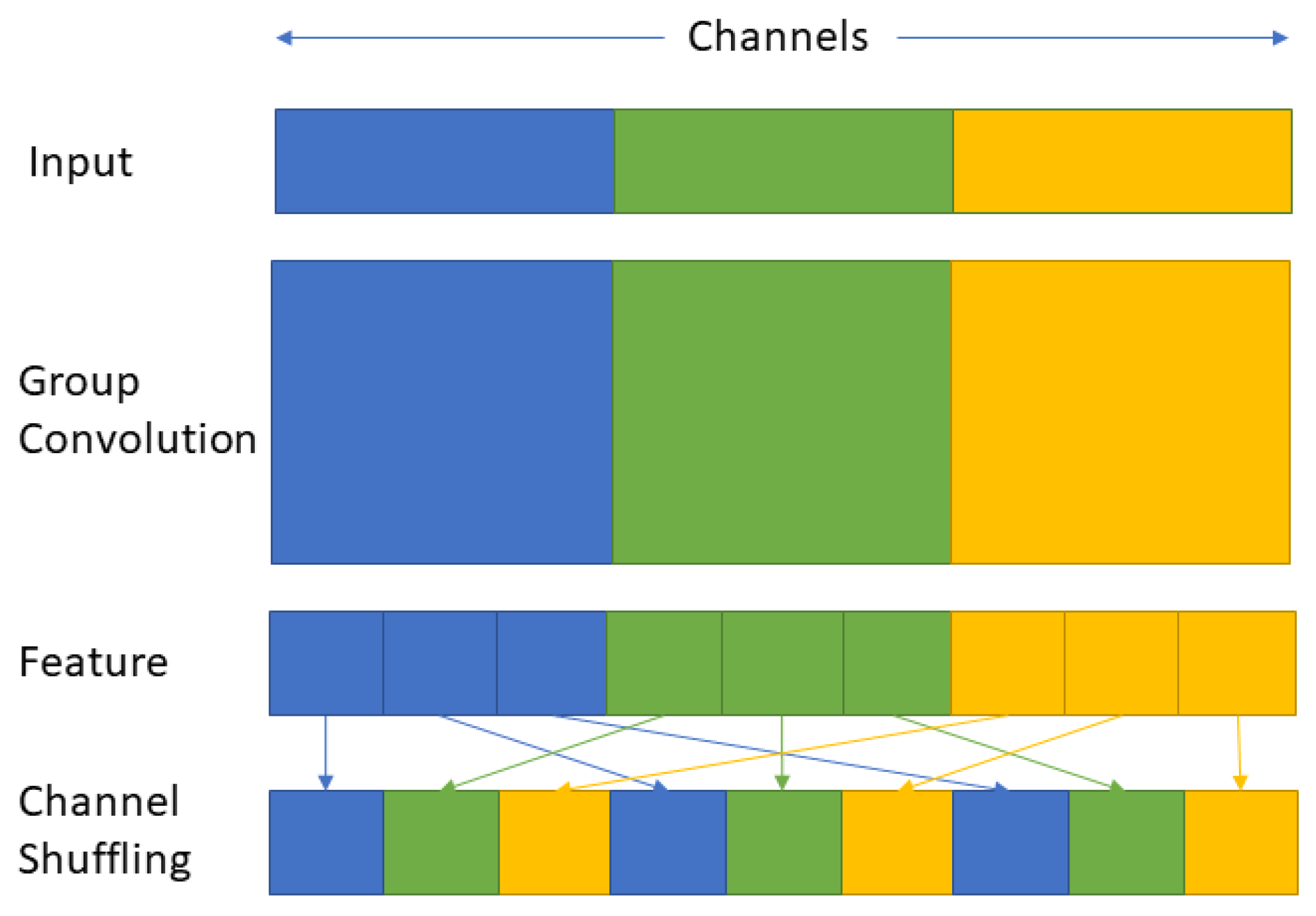
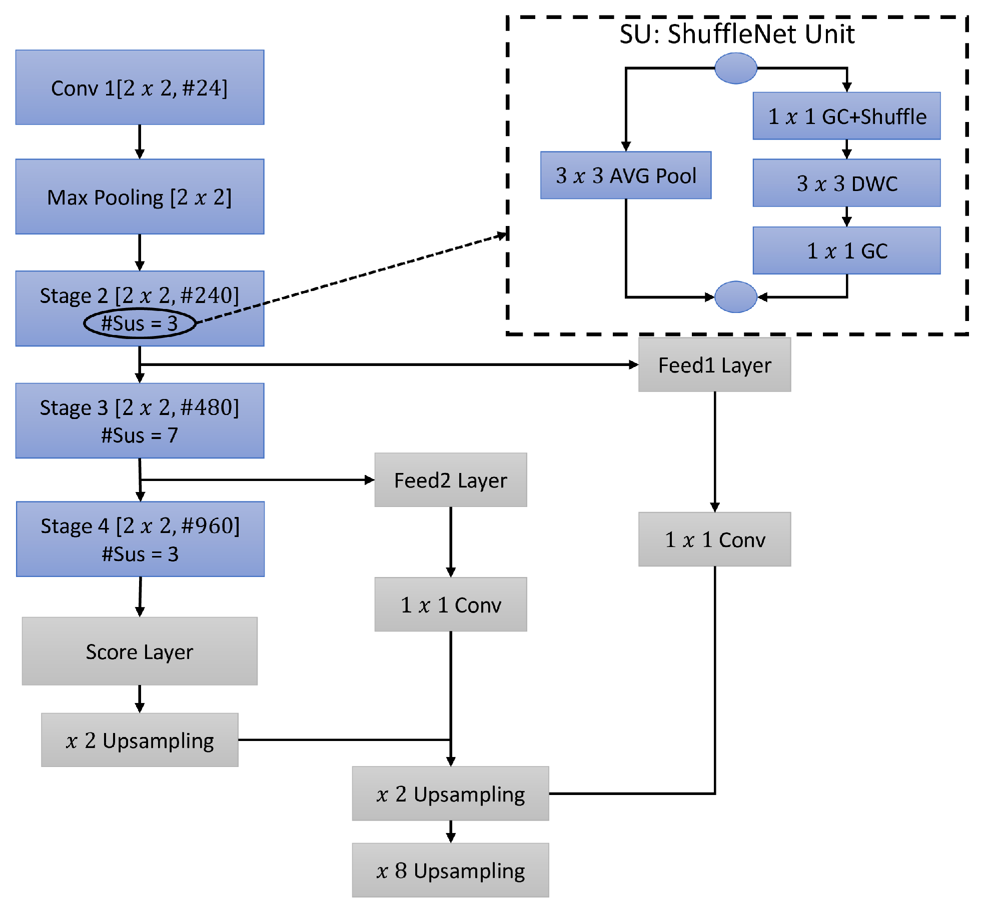
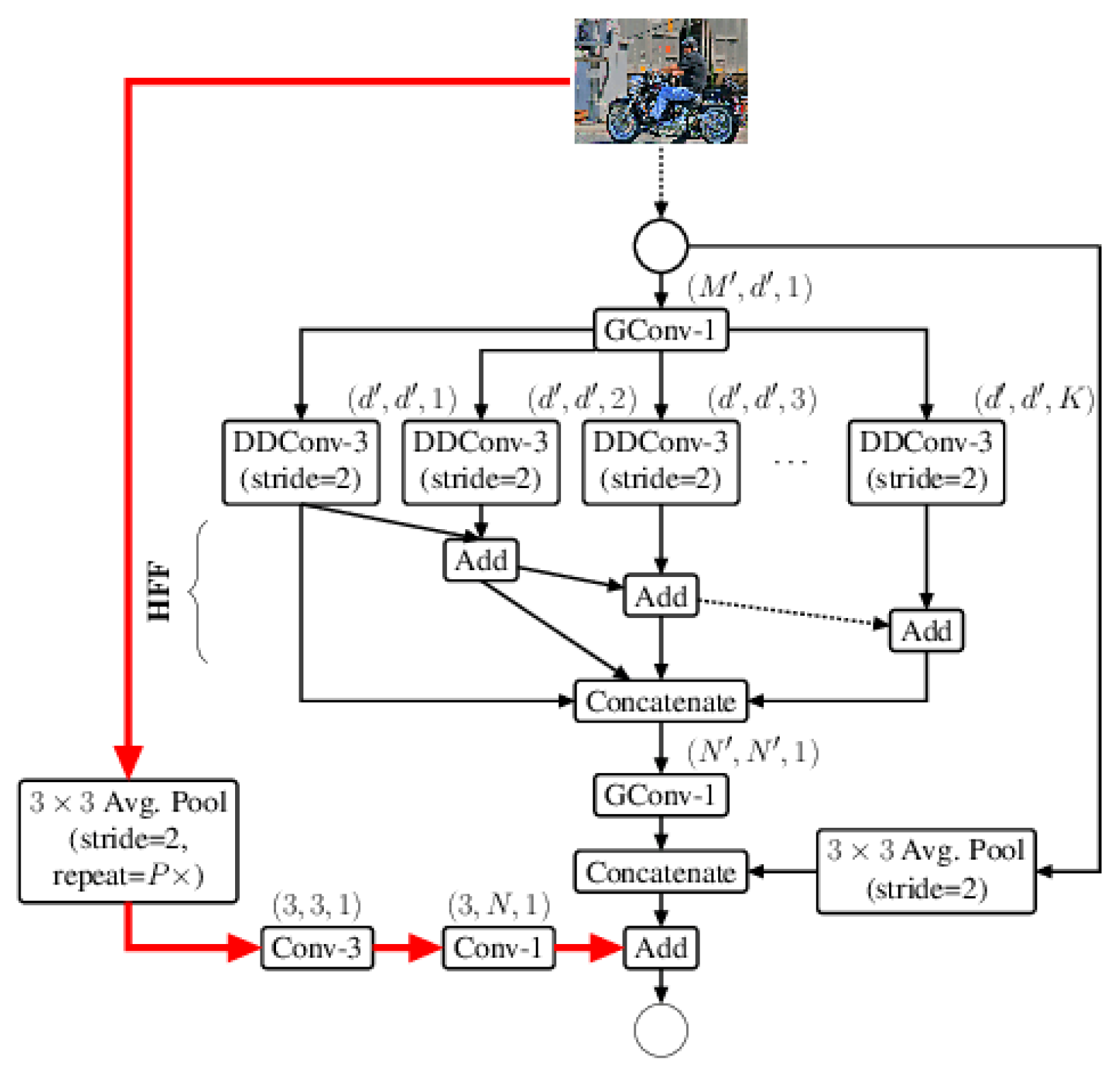
2.2. Channel Shuffling
2.3. Early Downsampling
2.4. The Use of Small Size Decoders
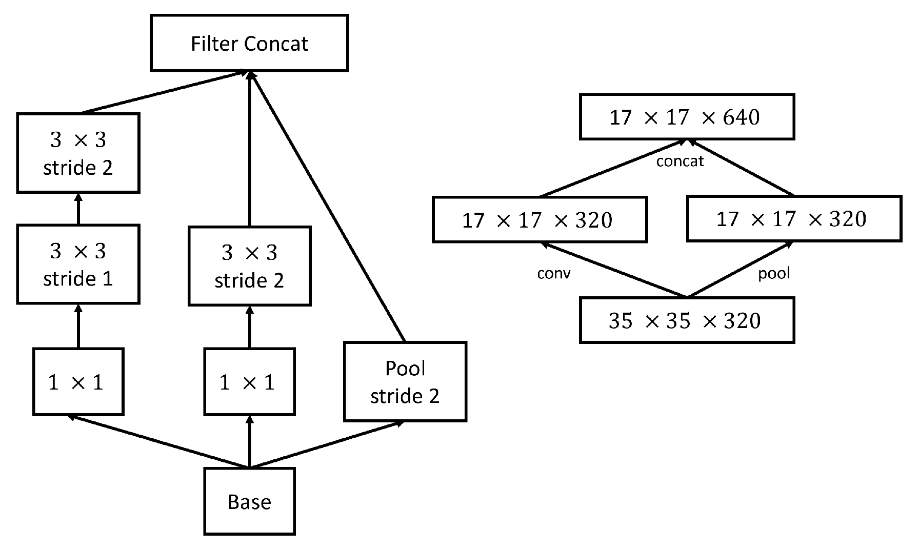
2.5. Efficient Reduction of the Feature Maps’ Grid Size
2.6. Increasing Network Depth While Decreasing Kernel Size
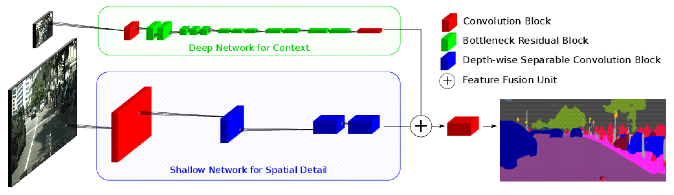
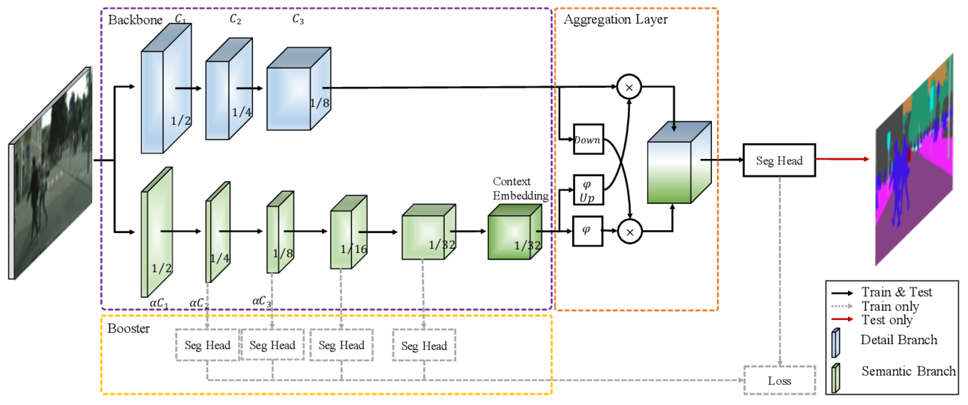
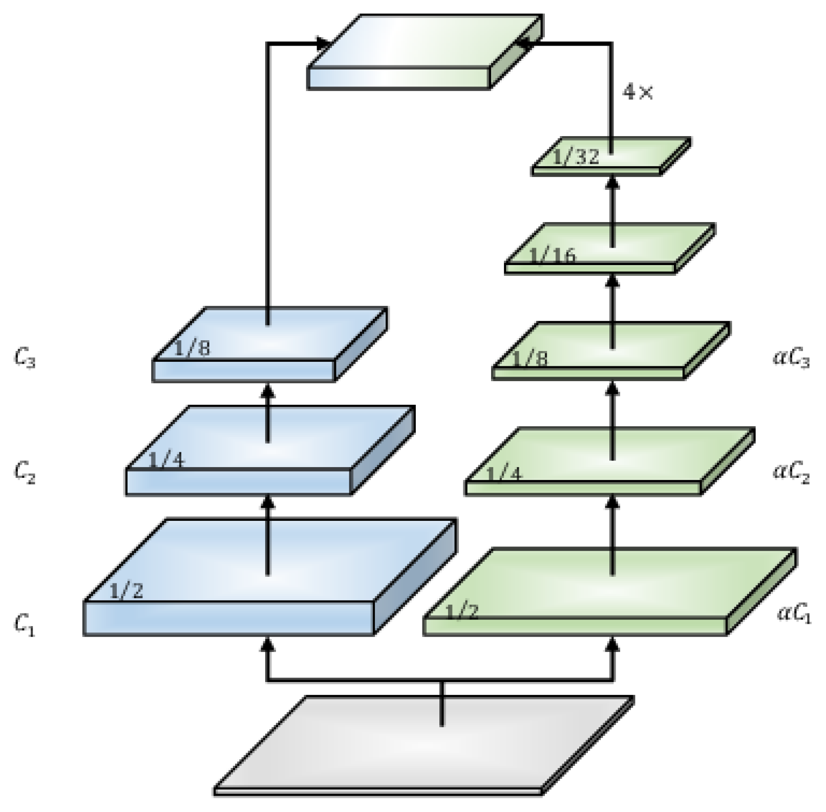
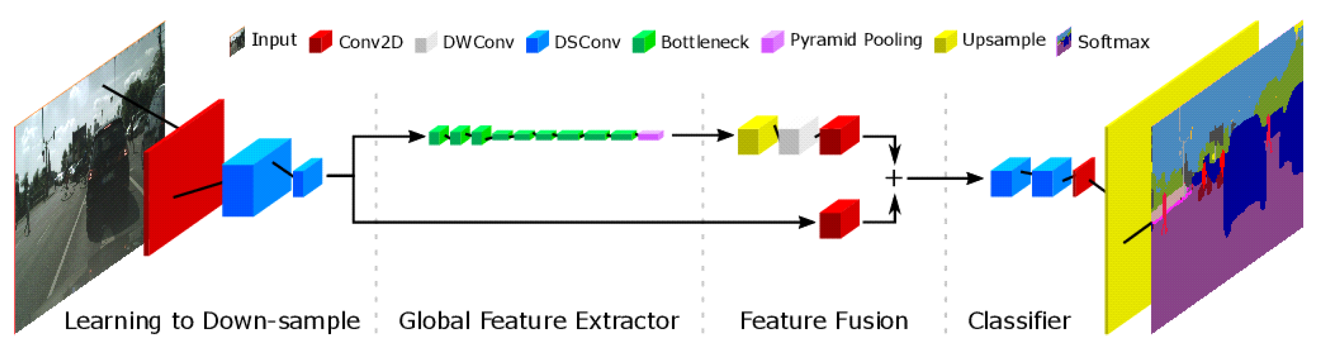
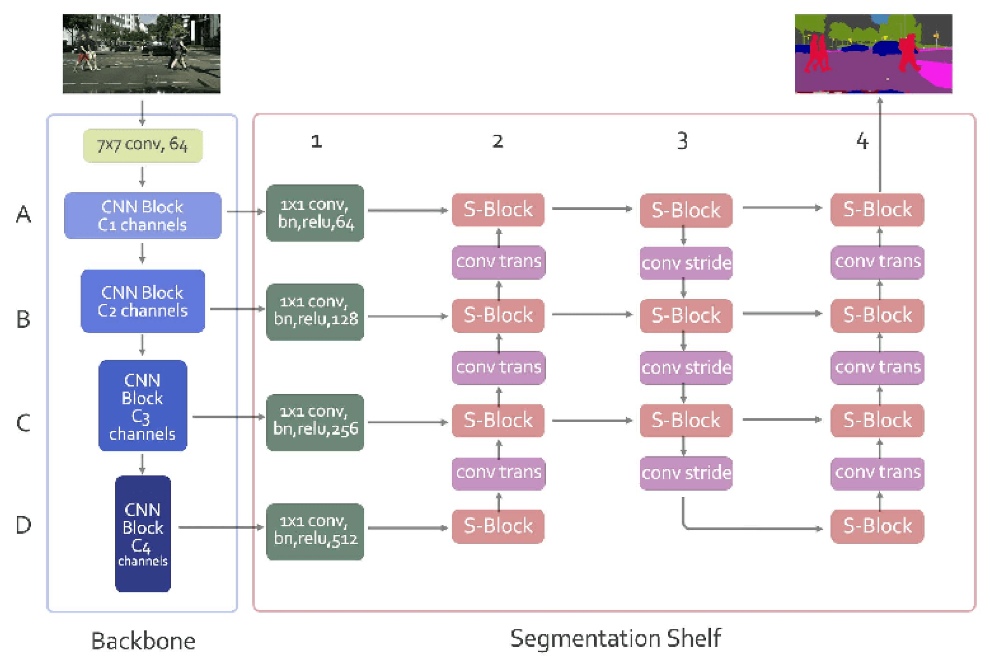
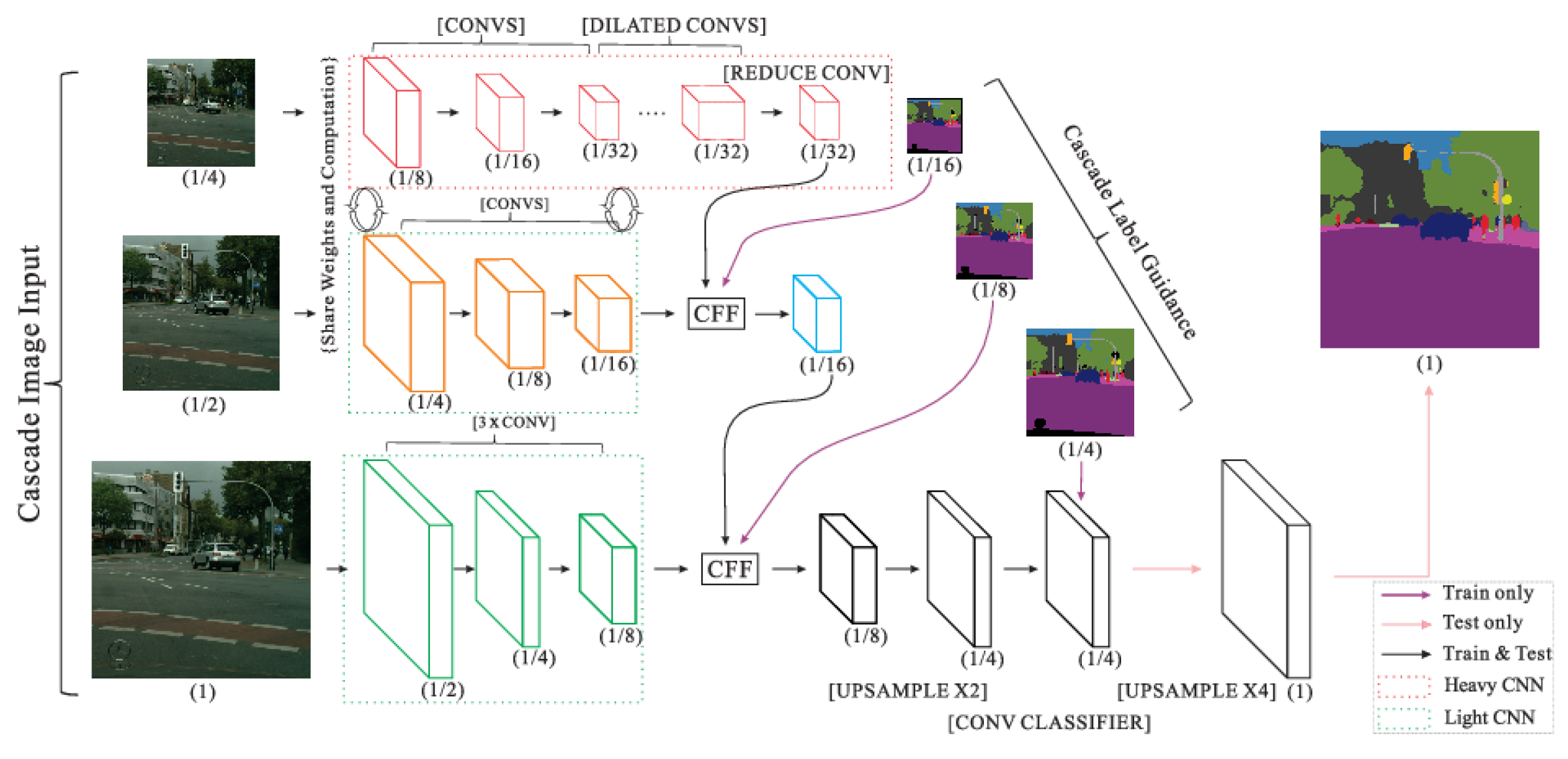
2.7. Two-Branch Networks
2.8. Block-Based Processing with Convolutional Neural Networks
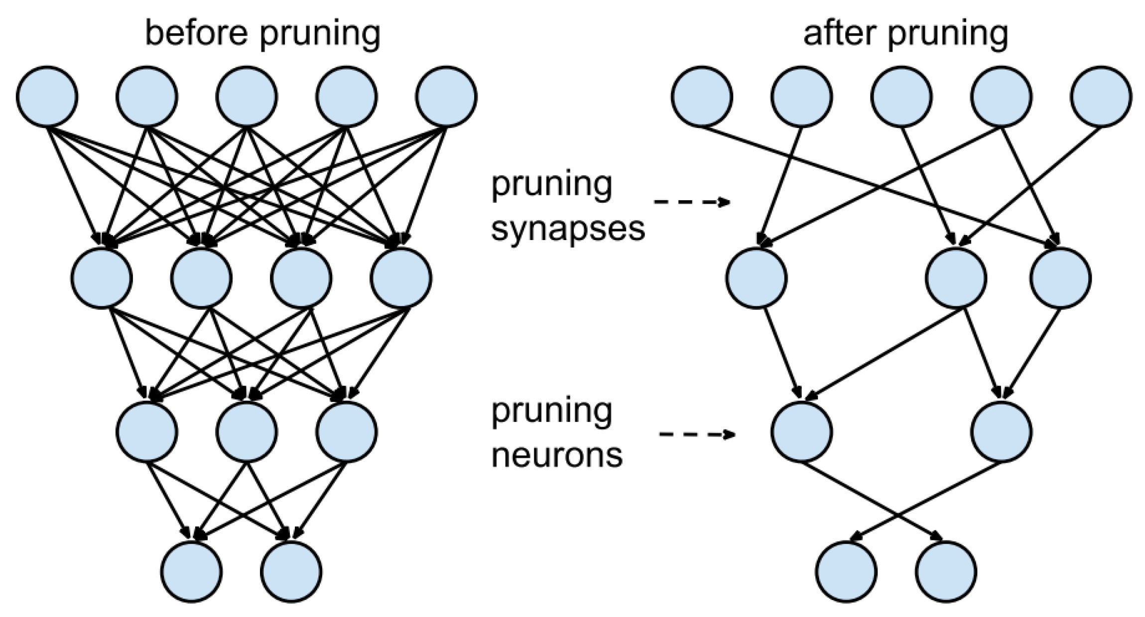
2.9. Pruning
2.10. Quantization
3. State-of-the-Art Deep-Learning Models
4. Evaluation Framework
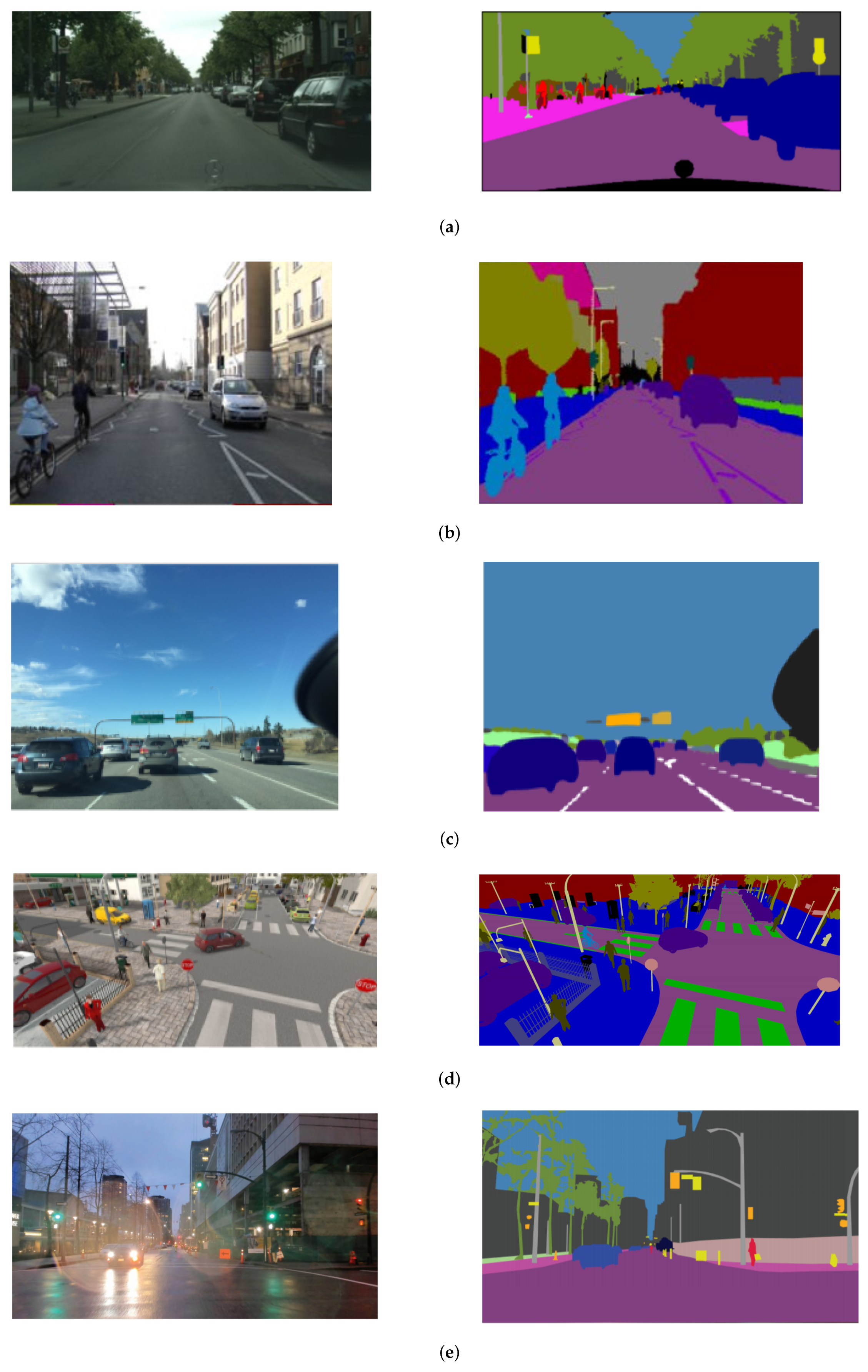
4.1. Datasets
4.1.1. Cityscapes
4.1.2. CamVid
4.1.3. MS COCO—Common Objects in Context
4.1.4. KITTI
4.1.5. KITTI-360
4.1.6. SYNTHIA
4.1.7. Mapillary Vistas
4.1.8. ApolloScape
4.1.9. RaidaR
4.2. Metrics
4.2.1. Metrics Related to Effectiveness
- Pixel Accuracy: is defined as the ratio of correctly classified pixels divided by their total number.
- Mean Pixel Accuracy: is an extension of Pixel Accuracy, which calculates the ratio of correct pixels in a per-class basis and then averaged over the total number of classes.
- Intersection over Union (IoU): is a very popular metric used in the field of semantic image segmentation. IoU is defined the intersection of the predicted segmentation map and the ground truth, divided by the area of union between the predicted segmentation map and the ground truth.
- mean Intersection over Union (mIoU): is the most widely used metric for semantic segmentation. It is defined as the average IoU over all classes.
4.2.2. Metrics Related to Efficiency
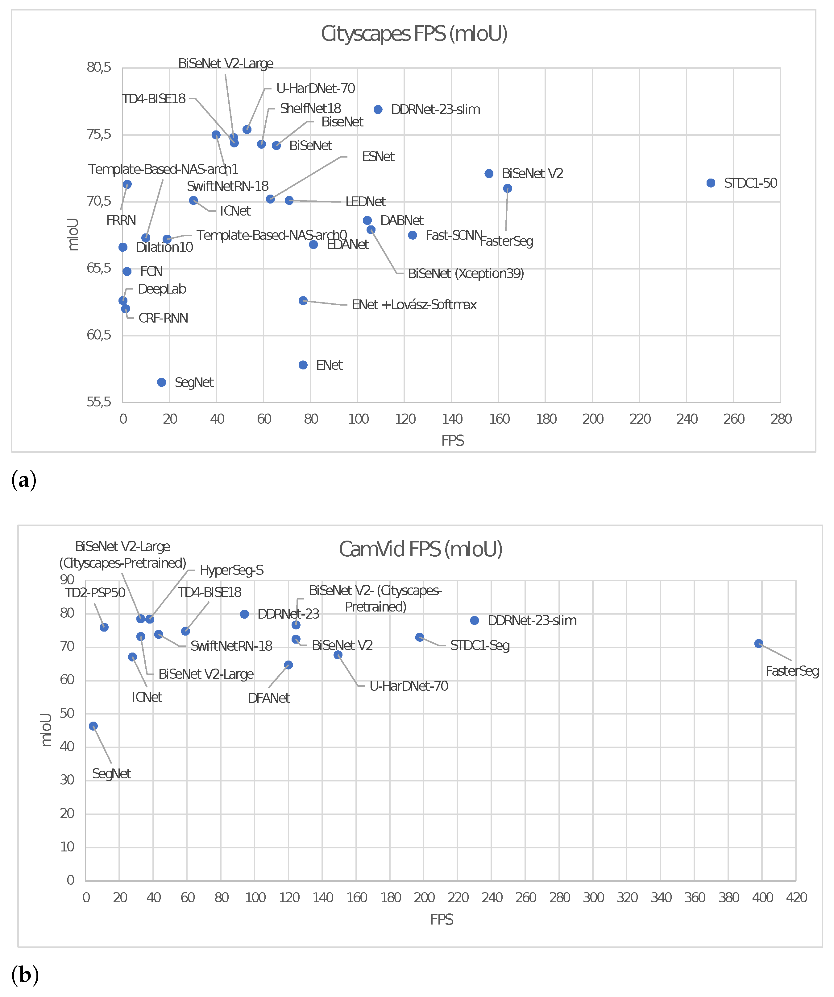
- Frames per second: A standard metric for evaluating the time needed for a deep-learning model to process a series of image frames of a video is “Frames per second”. Especially in real-time semantic segmentation applications, such as autonomous driving, it is crucial to know the exact number of frames a model can process below the time of a second. It is a very popular metric, and it can be really helpful for comparing different segmentation methods and architectures.
- Inference time: is another standard metric for evaluating the speed of semantic segmentation. It is the inverse of FPS (Frame Rate), and it measures the execution time for a frame.
- Memory usage: it is also a significant parameter to be taken into consideration when comparing deep-learning models in terms of speed and efficiency. Memory usage can be measured in different ways. Some researchers use the number of parameters of the network. Another way is to define the memory size to represent the network and lastly, a metric used frequently is to measure the number of floating-point operations (FLOPs) required for the execution.
5. Discussion
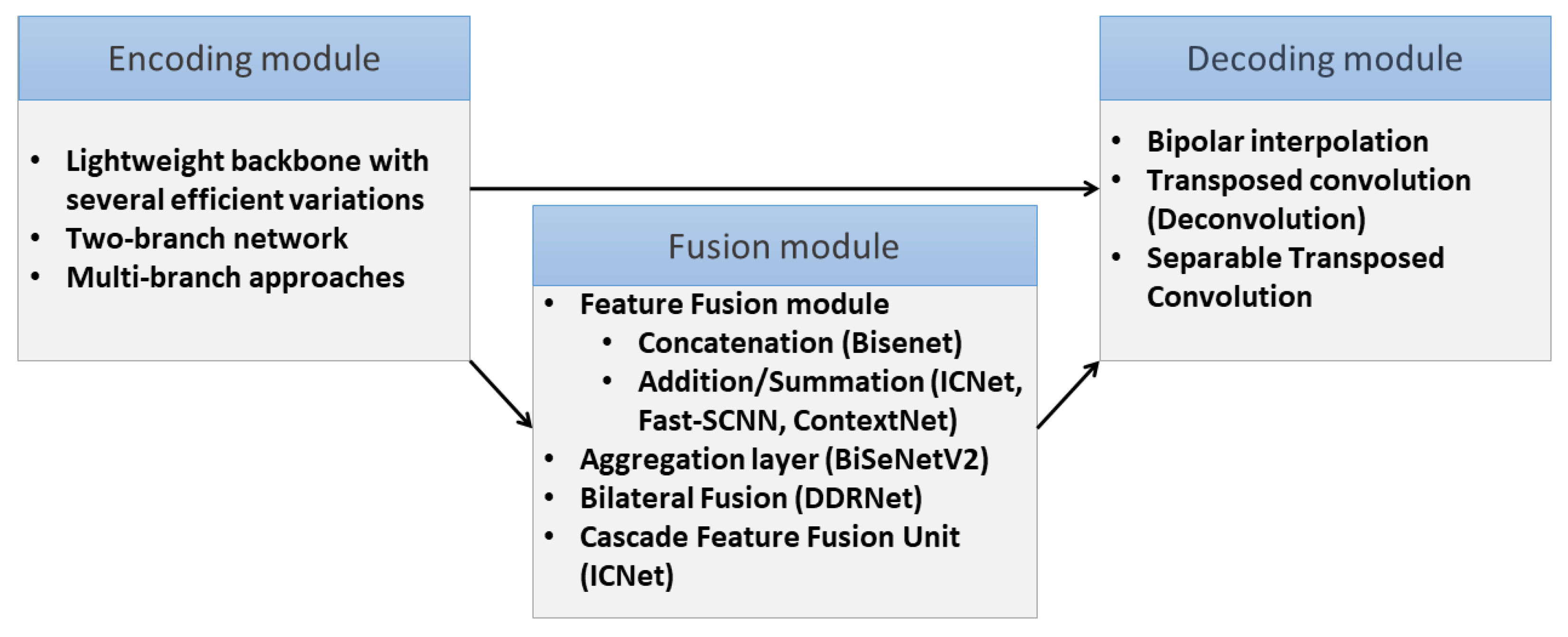
5.1. Common Operational Pipeline
5.2. Comparative Performance Analysis
5.2.1. Dataset-Oriented Performance
5.2.2. The Influence of Hardware
6. Future Research Trends
- Transfer learning: Transfer learning transfers the knowledge (i.e., weights) from the source domain to the target domain, leading to a great positive effect on many domains that are difficult to improve because of insufficient training data [66]. By the same token, transfer learning can be useful in real-time semantic segmentation by reducing the amount of the needed training data, therefore the time required. Moreover, as [47] proposes, transfer learning offers a greater regularization to the parameters of a pre-trained model. In [67,68], the use of transfer learning improved the semantic segmentation performance in terms of accuracy.
- Domain adaptation: Domain adaptation is a subset of transfer learning. Domain adaptation’s goal is to ameliorate the model’s effectiveness on a target domain using the knowledge learned in a different, yet coherent source domain [69]. In [70] the use of domain adaptation, achieved a satisfactory increase in mIoU on unseen data, without the adding extra computational burden, which is one of the great goals of real-time semantic segmentation. Thus, domain adaptation might be a valuable solution for the future of autonomous driving, by giving accurate results on unseen domains while functioning in low latency.
- Self-supervised learning: Human-crafting large-scale data has a high cost, is time-consuming and sometimes is an almost impracticable process. Especially in the field of autonomous driving, where millions of data are required due to the complexity of the street scenes, many hurdles arise in the annotation of the data. Self-supervised learning is a subcategory of unsupervised learning introduced to learn representations from extensive datasets without providing manually labeled data. Thus, any human actions (and involvements) are avoided, reducing the operational costs [71].
- Weakly supervised learning: Weakly supervised learning is related to learning methods which are characterized by coarse-grained labels or inaccurate labels. As reported in [71], the cost of obtaining weak supervision labels is generally much cheaper than fine-grained labels for supervised methods. In [72], a superior performance compared to other methods has been achieved in terms of accuracy, for a benchmark that uses the “Cityscapes” and “CamVid” datasets. Additionally, ref. [73] with the use of classifier heatmaps and a two-stream network shows greater performance in comparison to the other state-of-the-art models that use additional supervision.
- Transformers: ref. [74] allows the modeling of a global context already at the first layer and throughout the network, contrary to the ordinary convolutional-based methods. Segmenter approach reaches a mean IoU of 50.77% on ADE20K [75], surpassing all previous state-of-the-art convolutional approaches by a gap of 4.6%. Thus, transformers appear to be promising methods for the future of semantic segmentation.
7. Conclusions
Author Contributions
Funding
Acknowledgments
Conflicts of Interest
References
- Janai, J.; Güney, F.; Behl, A.; Geiger, A. Computer Vision for Autonomous Vehicles: Problems, Datasets and State of the Art. Found. Trends Comput. Graph. Vis. 2020, 12, 85. [Google Scholar] [CrossRef]
- Wang, M.; Liu, B.; Foroosh, H. Factorized Convolutional Neural Networks. In Proceedings of the 2017 IEEE International Conference on Computer Vision Workshops (ICCVW), Venice, Italy, 22–29 October 2017; pp. 545–553. [Google Scholar] [CrossRef]
- Guo, Y.; Li, Y.; Feris, R.; Wang, L.; Simunic, T. Depthwise Convolution Is All You Need for Learning Multiple Visual Domains; AAAI: Honolulu, HI, USA, 2019. [Google Scholar]
- Chollet, F. Xception: Deep Learning with Depthwise Separable Convolutions. In Proceedings of the 2017 IEEE Conference on Computer Vision and Pattern Recognition (CVPR), Honolulu, HI, USA, 21–26 July 2017; pp. 1800–1807. [Google Scholar]
- Szegedy, C.; Liu, W.; Jia, Y.; Sermanet, P.; Reed, S.E.; Anguelov, D.; Erhan, D.; Vanhoucke, V.; Rabinovich, A. Going deeper with convolutions. In Proceedings of the 2015 IEEE Conference on Computer Vision and Pattern Recognition (CVPR), Boston, MA, USA, 7–12 June 2015; pp. 1–9. [Google Scholar]
- Howard, A.G.; Zhu, M.; Chen, B.; Kalenichenko, D.; Wang, W.; Weyand, T.; Andreetto, M.; Adam, H. MobileNets: Efficient Convolutional Neural Networks for Mobile Vision Applications. arXiv 2017, arXiv:abs/1704.04861. [Google Scholar]
- Zhang, X.; Zhou, X.; Lin, M.; Sun, J. ShuffleNet: An Extremely Efficient Convolutional Neural Network for Mobile Devices. arXiv 2017, arXiv:cs.CV/1707.01083. [Google Scholar]
- Paszke, A.; Chaurasia, A.; Kim, S.; Culurciello, E. ENet: A Deep Neural Network Architecture for Real-Time Semantic Segmentation. arXiv 2016, arXiv:abs/1606.02147. [Google Scholar]
- Badrinarayanan, V.; Kendall, A.; Cipolla, R. SegNet: A Deep Convolutional Encoder-Decoder Architecture for Image Segmentation. IEEE Trans. Pattern Anal. Mach. Intell. 2017, 39, 2481–2495. [Google Scholar] [CrossRef]
- Szegedy, C.; Vanhoucke, V.; Ioffe, S.; Shlens, J.; Wojna, Z. Rethinking the Inception Architecture for Computer Vision. In Proceedings of the 2016 IEEE Conference on Computer Vision and Pattern Recognition (CVPR), Las Vegas, NV, USA, 27–30 June 2016; pp. 2818–2826. [Google Scholar] [CrossRef] [Green Version]
- Fan, M.; Lai, S.; Huang, J.; Wei, X.; Chai, Z.; Luo, J.; Wei, X. Rethinking BiSeNet For Real-time Semantic Segmentation. arXiv 2021, arXiv:cs.CV/2104.13188. [Google Scholar]
- Simonyan, K.; Zisserman, A. Very Deep Convolutional Networks for Large-Scale Image Recognition. arXiv 2014, arXiv:1409.1556. [Google Scholar]
- Nekrasov, V.; Shen, C.; Reid, I. Template-Based Automatic Search of Compact Semantic Segmentation Architectures. In 2020 IEEE Winter Conference on Applications of Computer Vision (WACV); IEEE: Los Alamitos, CA, USA, 2020. [Google Scholar]
- Yu, C.; Wang, J.; Peng, C.; Gao, C.; Yu, G.; Sang, N. BiSeNet: Bilateral Segmentation Network for Real-Time Semantic Segmentation; Computer Vision–ECCV 2018; Ferrari, V., Hebert, M., Sminchisescu, C., Weiss, Y., Eds.; Springer International Publishing: Cham, Switzerland, 2018; pp. 334–349. [Google Scholar]
- Yu, C.; Gao, C.; Wang, J.; Yu, G.; Shen, C.; Sang, N. BiSeNet V2: Bilateral Network with Guided Aggregation for Real-time Semantic Segmentation. arXiv 2020, arXiv:abs/2004.02147. [Google Scholar]
- Hong, Y.; Pan, H.; Sun, W.; Jia, Y. Deep Dual-resolution Networks for Real-time and Accurate Semantic Segmentation of Road Scenes. arXiv 2021, arXiv:abs/2101.06085. [Google Scholar]
- Verelst, T.; Tuytelaars, T. SegBlocks: Block-Based Dynamic Resolution Networks for Real-Time Segmentation. arXiv 2020, arXiv:abs/2011.12025. [Google Scholar]
- Han, S.; Pool, J.; Tran, J.; Dally, W. Learning both Weights and Connections for Efficient Neural Network. arXiv 2015, arXiv:abs/1506.02626. [Google Scholar]
- Han, S.; Mao, H.; Dally, W. Deep Compression: Compressing Deep Neural Network with Pruning, Trained Quantization and Huffman Coding. arXiv 2016, arXiv:1510.00149. [Google Scholar]
- Li, H.; Kadav, A.; Durdanovic, I.; Samet, H.; Graf, H.P. Pruning Filters for Efficient ConvNets. arXiv 2017, arXiv:cs.CV/1608.08710. [Google Scholar]
- He, Y.; Zhang, X.; Sun, J. Channel Pruning for Accelerating Very Deep Neural Networks. In Proceedings of the 2017 IEEE International Conference on Computer Vision (ICCV), Venice, Italy, 22–29 October 2017; pp. 1398–1406. [Google Scholar]
- Takos, G. A Survey on Deep Learning Methods for Semantic Image Segmentation in Real-Time. arXiv 2020, arXiv:abs/2009.12942. [Google Scholar]
- Wu, Z.; Shen, C.; van den Hengel, A. Real-time Semantic Image Segmentation via Spatial Sparsity. arXiv 2017, arXiv:cs.CV/1712.00213. [Google Scholar]
- Poudel, R.P.K.; Bonde, U.D.; Liwicki, S.; Zach, C. ContextNet: Exploring Context and Detail for Semantic Segmentation in Real-Time; BMVC: Newcastle, UK, 2018. [Google Scholar]
- Poudel, R.P.K.; Liwicki, S.; Cipolla, R. Fast-SCNN: Fast Semantic Segmentation Network. arXiv 2019, arXiv:cs.CV/1902.04502. [Google Scholar]
- Sandler, M.; Howard, A.; Zhu, M.; Zhmoginov, A.; Chen, L.C. MobileNetV2: Inverted Residuals and Linear Bottlenecks. In Proceedings of the 2018 IEEE/CVF Conference on Computer Vision and Pattern Recognition, Salt Lake City, UT, USA, 18–23 June 2018; pp. 4510–4520. [Google Scholar] [CrossRef] [Green Version]
- Chen, W.; Gong, X.; Liu, X.; Zhang, Q.; Li, Y.; Wang, Z. FasterSeg: Searching for Faster Real-time Semantic Segmentation. In Proceedings of the International Conference on Learning Representations, Addis Ababa, Ethiopia, 30 April 2020. [Google Scholar]
- Elsken, T.; Metzen, J.H.; Hutter, F. Neural Architecture Search: A Survey. J. Mach. Learn. Res. 2019, 20, 1–21. [Google Scholar]
- Elsken, T.; Metzen, J.H.; Hutter, F. Neural Architecture Search. In Automated Machine Learning: Methods, Systems, Challenges; Hutter, F., Kotthoff, L., Vanschoren, J., Eds.; Springer International Publishing: Cham, Switzerland, 2019; pp. 63–77. [Google Scholar]
- Liu, C.; Chen, L.C.; Schroff, F.; Adam, H.; Hua, W.; Yuille, A.; Li, F.-F. Auto-DeepLab: Hierarchical Neural Architecture Search for Semantic Image Segmentation. In Proceedings of the 2019 IEEE/CVF Conference on Computer Vision and Pattern Recognition (CVPR), Long Beach, CA, USA, 16–20 June 2019; pp. 82–92. [Google Scholar]
- Gou, J.; Yu, B.; Maybank, S.; Tao, D. Knowledge Distillation: A Survey. Int. J. Comput. Vis. 2021, 129, 1789–1819. [Google Scholar] [CrossRef]
- Wang, Y.; Zhou, Q.; Wu, X. ESNet: An Efficient Symmetric Network for Real-Time Semantic Segmentation; PRCV: Xi’an, China, 2019. [Google Scholar]
- Zhuang, J.; Yang, J.; Gu, L.; Dvornek, N. ShelfNet for Fast Semantic Segmentation. In Proceedings of the 2019 IEEE/CVF International Conference on Computer Vision Workshop (ICCVW), Seoul, Korea, 27–28 October 2019; pp. 847–856. [Google Scholar]
- Zhao, H.; Qi, X.; Shen, X.; Shi, J.; Jia, J. ICNet for Real-Time Semantic Segmentation on High-Resolution Images. In Computer Vision—ECCV 2018; Ferrari, V., Hebert, M., Sminchisescu, C., Weiss, Y., Eds.; Springer International Publishing: Cham, Switzerland, 2018; pp. 418–434. [Google Scholar]
- Bergman, A.W.; Lindell, D.B. Factorized Convolution Kernels in Image Processing; Stanford University: Stanford, CA, USA, 2019. [Google Scholar]
- Mehta, S.; Rastegari, M.; Caspi, A.; Shapiro, L.; Hajishirzi, H. ESPNet: Efficient Spatial Pyramid of Dilated Convolutions for Semantic Segmentation. In Computer Vision—ECCV 2018; Ferrari, V., Hebert, M., Sminchisescu, C., Weiss, Y., Eds.; Springer International Publishing: Cham, Switerland, 2018; pp. 561–580. [Google Scholar]
- Mehta, S.; Rastegari, M.; Shapiro, L.; Hajishirzi, H. ESPNetv2: A Light-Weight, Power Efficient, and General Purpose Convolutional Neural Network. In Proceedings of the 2019 IEEE/CVF Conference on Computer Vision and Pattern Recognition (CVPR), Long Beach, CA, USA, 16–20 June 2019; pp. 9182–9192. [Google Scholar] [CrossRef] [Green Version]
- Vallurupalli, N.; Annamaneni, S.; Varma, G.; Jawahar, C.V.; Mathew, M.; Nagori, S. Efficient Semantic Segmentation Using Gradual Grouping. In Proceedings of the 2018 IEEE/CVF Conference on Computer Vision and Pattern Recognition Workshops (CVPRW), Salt Lake City, UT, USA, 18–22 June 2018; pp. 711–7118. [Google Scholar]
- Li, G.; Yun, I.; Kim, J.; Kim, J. DABNet: Depth-Wise Asymmetric Bottleneck for Real-Time Semantic Segmentation; BMVC: Cardiff, UK, 2019. [Google Scholar]
- Li, H.; Xiong, P.; Fan, H.; Sun, J. DFANet: Deep Feature Aggregation for Real-Time Semantic Segmentation. In Proceedings of the 2019 IEEE/CVF Conference on Computer Vision and Pattern Recognition (CVPR), Long Beach, CA, USA, 16–20 June 2019; pp. 9514–9523. [Google Scholar]
- Gamal, M.; Siam, M.; Abdel-Razek, M. ShuffleSeg: Real-time Semantic Segmentation Network. arXiv 2018, arXiv:cs.CV/1803.03816. [Google Scholar]
- Chao, P.; Kao, C.; Ruan, Y.; Huang, C.; Lin, Y. HarDNet: A Low Memory Traffic Network. In Proceedings of the 2019 IEEE/CVF International Conference on Computer Vision (ICCV), Seoul, Korea, 27 October–2 November 2019; pp. 3551–3560. [Google Scholar] [CrossRef] [Green Version]
- Romera, E.; Álvarez, J.M.; Bergasa, L.M.; Arroyo, R. ERFNet: Efficient Residual Factorized ConvNet for Real-Time Semantic Segmentation. IEEE Trans. Intell. Transp. Syst. 2018, 19, 263–272. [Google Scholar] [CrossRef]
- Wang, Y.; Zhou, Q.; Liu, J.; Xiong, J.; Gao, G.; Wu, X.; Latecki, L. Lednet: A Lightweight Encoder-Decoder Network for Real-Time Semantic Segmentation. In Proceedings of the 2019 IEEE International Conference on Image Processing (ICIP), Taipei, Taiwan, 22–25 September 2019; pp. 1860–1864. [Google Scholar]
- Lo, S.Y.; Hang, H.; Chan, S.; Lin, J.J. Efficient Dense Modules of Asymmetric Convolution for Real-Time Semantic Segmentation. In Proceedings of the ACM Multimedia Asia, Beijing, China, 15–18 December 2019. [Google Scholar]
- Nirkin, Y.; Wolf, L.; Hassner, T. HyperSeg: Patch-wise Hypernetwork for Real-time Semantic Segmentation. arXiv 2020, arXiv:abs/2012.11582. [Google Scholar]
- Oršic, M.; Krešo, I.; Bevandic, P.; Šegvic, S. In Defense of Pre-Trained ImageNet Architectures for Real-Time Semantic Segmentation of Road-Driving Images. In Proceedings of the 2019 IEEE/CVF Conference on Computer Vision and Pattern Recognition (CVPR), Long Beach, CA, USA, 16–20 June 2019; pp. 12599–12608. [Google Scholar] [CrossRef] [Green Version]
- Hu, P.; Caba, F.; Wang, O.; Lin, Z.; Sclaroff, S.; Perazzi, F. Temporally Distributed Networks for Fast Video Semantic Segmentation. In Proceedings of the 2020 IEEE/CVF Conference on Computer Vision and Pattern Recognition (CVPR), Seattle, WA, USA, 13–19 June 2020; pp. 8815–8824. [Google Scholar] [CrossRef]
- Treml, M.; Arjona-Medina, J.; Unterthiner, T.; Durgesh, R.; Friedmann, F.; Schuberth, P.; Mayr, A.; Heusel, M.; Hofmarcher, M.; Widrich, M.; et al. Speeding up Semantic Segmentation for Autonomous Driving. In Proceedings of the 2016 Machine Learning for Intelligent Transportation Systems (MLITS) in Conjunction with the Thirtieth Conference on Neural Information Processing Systems (NIPS), Barcelona, Spain, 5–10 December 2016. [Google Scholar]
- Chaurasia, A.; Culurciello, E. LinkNet: Exploiting encoder representations for efficient semantic segmentation. In Proceedings of the 2017 IEEE Visual Communications and Image Processing (VCIP), St. Petersburg, FL, USA, 10–13 December 2017; pp. 1–4. [Google Scholar] [CrossRef] [Green Version]
- DSNet for Real-Time Driving Scene Semantic Segmentation. arXiv 2018, arXiv:abs/1812.07049.
- Nekrasov, V.; Shen, C.; Reid, I.D. Light-Weight RefineNet for Real-Time Semantic Segmentation. arXiv 2018, arXiv:abs/1810.03272. [Google Scholar]
- Emara, T.; Munim, H.E.A.E.; Abbas, H.M. LiteSeg: A Novel Lightweight ConvNet for Semantic Segmentation. In Proceedings of the 2019 Digital Image Computing: Techniques and Applications (DICTA), Perth, Australia, 2–4 December 2019; pp. 1–7. [Google Scholar] [CrossRef] [Green Version]
- Berman, M.; Triki, A.; Blaschko, M.B. The Lovasz-Softmax Loss: A Tractable Surrogate for the Optimization of the Intersection-Over-Union Measure in Neural Networks. In Proceedings of the 2018 IEEE/CVF Conference on Computer Vision and Pattern Recognition, Salt Lake City, UT, USA, 18–23 June 2018; pp. 4413–4421. [Google Scholar]
- Cordts, M.; Omran, M.; Ramos, S.; Rehfeld, T.; Enzweiler, M.; Benenson, R.; Franke, U.; Roth, S.; Schiele, B. The Cityscapes Dataset for Semantic Urban Scene Understanding. In Proceedings of the 2016 IEEE Conference on Computer Vision and Pattern Recognition (CVPR), Las Vegas, NV, USA, 27–30 June 2016; pp. 3213–3223. [Google Scholar]
- Brostow, G.J.; Fauqueur, J.; Cipolla, R. Semantic object classes in video: A high-definition ground truth database. Pattern Recognit. Lett. 2009, 30, 88–97. [Google Scholar] [CrossRef]
- Lin, T.Y.; Maire, M.; Belongie, S.; Hays, J.; Perona, P.; Ramanan, D.; Dollár, P.; Zitnick, C.L. Microsoft COCO: Common Objects in Context. In Computer Vision—ECCV 2014; Fleet, D., Pajdla, T., Schiele, B., Tuytelaars, T., Eds.; Springer International Publishing: Cham, Switzerland, 2014; pp. 740–755. [Google Scholar]
- Geiger, A.; Lenz, P.; Stiller, C.; Urtasun, R. Vision meets robotics: The KITTI dataset. Int. J. Robot. Res. 2013, 32, 1231–1237. [Google Scholar] [CrossRef] [Green Version]
- Xie, J.; Kiefel, M.; Sun, M.T.; Geiger, A. Semantic Instance Annotation of Street Scenes by 3D to 2D Label Transfer. In Proceedings of the Conference on Computer Vision and Pattern Recognition (CVPR), Las Vegas, NV, USA, 27–30 June 2016. [Google Scholar]
- Ros, G.; Sellart, L.; Materzynska, J.; Vazquez, D.; Lopez, A.M. The SYNTHIA Dataset: A Large Collection of Synthetic Images for Semantic Segmentation of Urban Scenes. In Proceedings of the 2016 IEEE Conference on Computer Vision and Pattern Recognition (CVPR), Las Vegas, NV, USA, 27–30 June 2016; pp. 3234–3243. [Google Scholar] [CrossRef]
- Neuhold, G.; Ollmann, T.; Bulò, S.R.; Kontschieder, P. The Mapillary Vistas Dataset for Semantic Understanding of Street Scenes. In Proceedings of the 2017 IEEE International Conference on Computer Vision (ICCV), Venice, Italy, 22–29 October 2017; pp. 5000–5009. [Google Scholar] [CrossRef]
- Wang, P.; Huang, X.; Cheng, X.; Zhou, D.; Geng, Q.; Yang, R. The ApolloScape Open Dataset for Autonomous Driving and Its Application. IEEE Trans. Pattern Anal. Mach. Intell. 2020, 42, 2702–2719. [Google Scholar] [CrossRef] [PubMed] [Green Version]
- Jin, J.; Fatemi, A.; Lira, W.P.; Yu, F.; Leng, B.; Ma, R.; Mahdavi-Amiri, A.; Zhang, H.R. RaidaR: A Rich Annotated Image Dataset of Rainy Street Scenes. arXiv 2021, arXiv:abs/2104.04606. [Google Scholar]
- Garcia-Garcia, A.; Orts-Escolano, S.; Oprea, S.; Villena-Martinez, V.; Martinez-Gonzalez, P.; Garcia-Rodriguez, J. A survey on deep learning techniques for image and video semantic segmentation. Appl. Soft Comput. J. 2018, 70, 41–65. [Google Scholar] [CrossRef]
- Faniadis, E.; Amanatiadis, A. Deep Learning Inference at the Edge for Mobile and Aerial Robotics. In Proceedings of the 2020 IEEE International Symposium on Safety, Security, and Rescue Robotics (SSRR), Abu Dhabi, United Arab Emerites, 4–6 November 2020; pp. 334–340. [Google Scholar] [CrossRef]
- Tan, C.; Sun, F.; Kong, T.; Zhang, W.; Yang, C.; Liu, C. A Survey on Deep Transfer Learning. In Artificial Neural Networks and Machine Learning—ICANN 2018; Kůrková, V., Manolopoulos, Y., Hammer, B., Iliadis, L., Maglogiannis, I., Eds.; Springer International Publishing: Cham, Switzerland, 2018; pp. 270–279. [Google Scholar]
- Ye, J.; Lu, C.; Xiong, J.; Wang, H. Semantic Segmentation Algorithm Based on Attention Mechanism and Transfer Learning. Math. Probl. Eng. 2020, 2020, 1–11. [Google Scholar]
- Sharma, S.; Ball, J.E.; Tang, B.; Carruth, D.W.; Doude, M.; Islam, M.A. Semantic Segmentation with Transfer Learning for Off-Road Autonomous Driving. Sensors 2019, 19, 2577. [Google Scholar] [CrossRef] [Green Version]
- Csurka, G. Deep Visual Domain Adaptation. In Proceedings of the 2020 22nd International Symposium on Symbolic and Numeric Algorithms for Scientific Computing (SYNASC), Timisoara, Romania, 1–4 September 2020; pp. 1–8. [Google Scholar] [CrossRef]
- Sankaranarayanan, S.; Balaji, Y.; Jain, A.; Lim, S.N.; Chellappa, R. Learning from Synthetic Data: Addressing Domain Shift for Semantic Segmentation. In Proceedings of the 2018 IEEE/CVF Conference on Computer Vision and Pattern Recognition, Salt Lake City, UT, USA, 18–23 June 2018; pp. 3752–3761. [Google Scholar]
- Jing, L.; Tian, Y. Self-supervised Visual Feature Learning with Deep Neural Networks: A Survey. IEEE Trans. Pattern Anal. Mach. Intell. 2020. [Google Scholar] [CrossRef] [PubMed]
- Wang, X.; Ma, H.; You, S. Deep clustering for weakly-supervised semantic segmentation in autonomous driving scenes. Neurocomputing 2020, 381, 20–28. [Google Scholar] [CrossRef]
- Saleh, F.S.; Aliakbarian, M.S.; Salzmann, M.; Petersson, L.; Alvarez, J.M. Bringing Background into the Foreground: Making All Classes Equal in Weakly-Supervised Video Semantic Segmentation. In Proceedings of the 2017 IEEE International Conference on Computer Vision (ICCV), Venice, Italy, 22–29 October 2017; pp. 2125–2135. [Google Scholar] [CrossRef] [Green Version]
- Strudel, R.; Garcia, R.; Laptev, I.; Schmid, C. Segmenter: Transformer for Semantic Segmentation. arXiv 2021, arXiv:cs.CV/2105.05633. [Google Scholar]
- Zhou, B.; Zhao, H.; Puig, X.; Fidler, S.; Barriuso, A.; Torralba, A. Scene Parsing through ADE20K Dataset. In Proceedings of the 2017 IEEE Conference on Computer Vision and Pattern Recognition (CVPR), Honolulu, HI, USA, 21–26 July 2017; pp. 5122–5130. [Google Scholar] [CrossRef]


| Layer | Type | Output Channel | Output Resolution |
|---|---|---|---|
| 1 | Downsampling block | 16 | 512 × 256 |
| 2 3–5 5–7 | Downsampling block 3 × Non-bt-1D 2 × Conv-module | 64 128 64 | 256 × 128 128 × 64 256 × 128 |
| 8 9 10 11 12 13 14 15 16 | Downsampling block Non-bt-1d (dilated 2) Non-bt-1d (dilated 4) Non-bt-1d (dilated 8) Non-bt-1d (dilated 16) Conv-module (dilated 2) Conv-module (dilated 4) Conv-module (dilated 8) Conv-module (dilated 16) | 128 128 128 128 128 128 128 128 128 | 128 × 64 128 × 64 28 × 64 128 × 64 128 × 64 128 × 64 128 × 64 128 × 64 128 × 64 |
| 17 18–19 | Deconvolution (upsampling) 2 × Non-bt-1D | 64 64 | 256 × 128 256 × 128 |
| 20 21–22 | Deconvolution (upsampling) 2 × Non-bt-1D | 16 16 | 512 × 256 5125 × 256 |
| 23 | Deconvolution (upsampling) | C | 1024 × 512 |
| Layer | Type | Output Channel | Output Resolution |
|---|---|---|---|
| 1 | Downsampling block | 16 | 512 × 256 |
| 2 3–5 5–7 | Downsampling block 3 × Non-bt-1D 2 × Conv-module | 64 128 64 | 256 × 128 128 × 64 256 × 128 |
| 8 9 10 11 12 13 14 15 16 | Downsampling block Non-bt-1d (dilated 2) Non-bt-1d (dilated 4) Non-bt-1d (dilated 8) Non-bt-1d (dilated 16) Conv-module (dilated 2) Conv-module (dilated 4) Conv-module (dilated 8) Conv-module (dilated 16) | 128 128 128 128 128 128 128 128 128 | 128 × 64 128 × 64 128 × 64 128 × 64 128 × 64 128 × 64 128 × 64 128 × 64 128 × 64 |
| 17 18–19 | Deconvolution (upsampling) 2 × Non-bt-1D | 64 64 | 256 × 128 256 × 128 |
| 20 21–22 | Deconvolution (upsampling) 2 × Non-bt-1D | 16 16 | 512 × 256 5125 × 256 |
| 23 | Deconvolution (upsampling) | C | 1024 × 512 |
| Networks | Backbone | Efficiency-Oriented Approaches |
|---|---|---|
| DDRNet [16] | ResNet | two-branch network |
| STDC1-50 [11] | STDC | feature map size reduction |
| single branch efficient decoder | ||
| U-HarDNet-70 [42] | DenseNet | depthwise separable convolutions |
| HyperSeg [46] | EfficientNet-B1 | pointwise convolutions |
| PSPNet | depthwise convolutions | |
| ResNet18 | small decoder size | |
| SwiftNetRN-18 [47] | ResNet-18 | small decoder size (lightweight decoder) |
| MobileNet V2 | ||
| BiSeNet V2 [15] | VGGnet | two-branch network fast-downsampling |
| Xception | ||
| MobileNet | ||
| TD4-BISE18 [48] | TDNet | Grouped convolutions |
| ShelfNet18 [33] | ResNet | multi-branch network channel reduction |
| Xception | ||
| DenseNet | ||
| BiSeNet [14] | Xception39 | two-branch network |
| ResNet18 | ||
| SegBlocks [17] | - | block-based processing |
| FasterSeg [27] | FasterSeg | multi-branch network |
| ESNet [32] | ESNet | multi-branch network |
| pointwise convolutions (factorized convolutions) | ||
| LEDNet [44] | ResNet | channel shuffling |
| ICNet [34] | image cascade network | multi-branch network |
| SQ [49] | SqueezeNet | decreased kernel size |
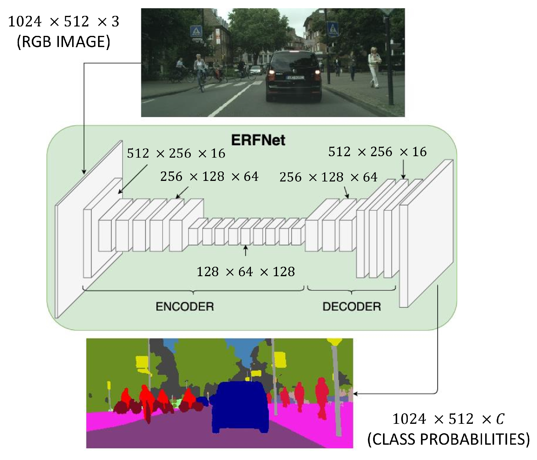
| ERFNet [43] | ERFNet | small decoder size |
| LinkNet [50] | ResNet18 | bypassing spatial information |
| SS [23] | ResNet18 | two-branch network |
| ContextNet [24] | ContextNet | two-branch network |
| depthwise separable convolutions | ||
| pruning | ||
| DSNet [51] | DSNet | channel shuffling |
| ESPNetv2 [37] | ESPNet | group pointwise convolutions |
| depthwise separable convolutions | ||
| ESSGG [38] | ERFNet | depthwise separable convolutions |
| channel shuffling | ||
| LWRF [52] | ResNet | decreasing kernel’s(receptive field) size |
| MobileNetV2 | small decoder size | |
| DABNet [39] | DABNet | depthwise separable convolutions |
| DFANet [40] | Xception | depthwise separable convolutions |
| Fast-SCNN [25] | Fast-SCNN | two-branch network |
| depthwise separable convolutions | ||
| ShuffleSeg [41] | ShuffleNet | Grouped convolutions |
| Channel shuffling | ||
| Template-Based-NAS-arch1 [13] | MobileNetV2 | separable convolutions |
| decreased kernel size | ||
| LiteSeg [53] | MobileNet | depthwise separable convolutions |
| ShuffleNet | ||
| DarkNet19 | ||
| Template-Based-NAS-arch0 [13] | MobileNetV2 | separable convolutions |
| decreased kernel size | ||
| ENet [8] | Enet | early downsampling |
| ResNets | small decoder size | |
| ENet + Lovász-Softmax [54] | - | early downsampling |
| small decoder size | ||
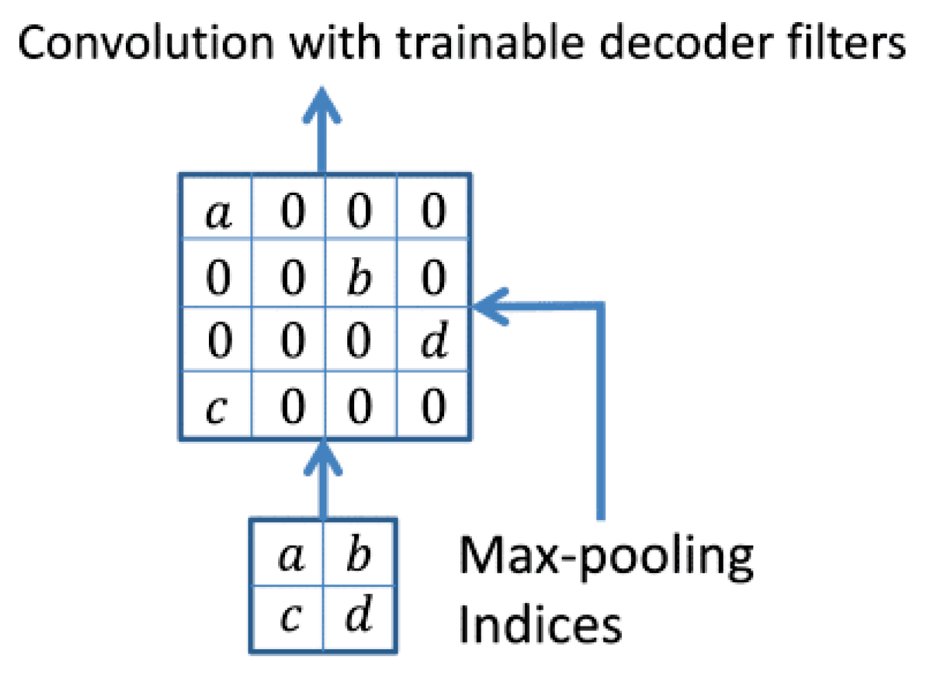
| SegNet [9] | VGG16 | reuse of max-pooling indices |
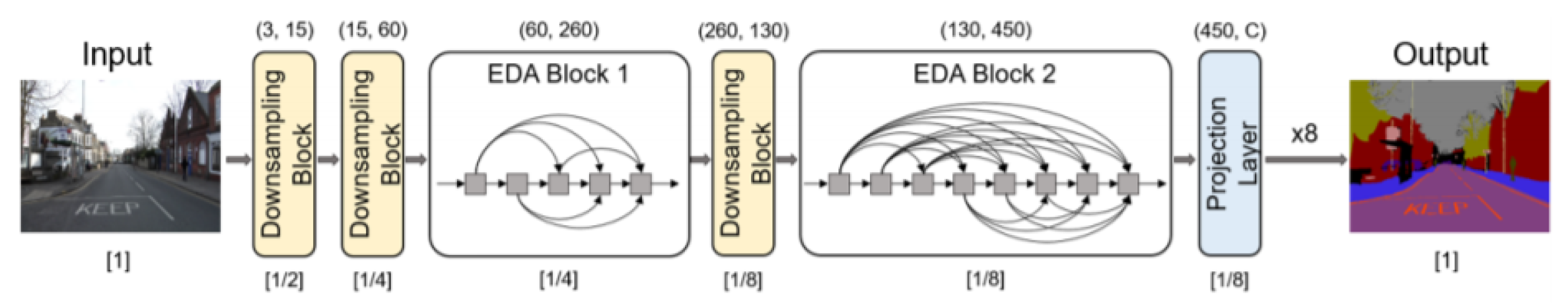
| EDANet [45] | EDA | early downsampling |
| factorized convolutions |
| Networks (Backbone) | Cityscapes | CamVid | ||||
|---|---|---|---|---|---|---|
| mIoU (%) | FPS | Hardware | mIoU (%) | FPS | Hardware | |
| SQ (SqueezeNet) | 84.3 | 16.7 | Jetson TX1 | - | - | - |
| DDRNet-23 | 79.4 | 38.5 | GTX 2080Ti | 79.9 | 94 | GTX 2080Ti |
| HyperSeg-S (EfficientNet-B1) | 78.1 | 16.1 | GTX 1080TI | 78.4 | 38.0 | GTX 1080TI |
| DDRNet-23-slim | 77.4 | 108.8 | GTX 2080Ti | 78.0 | 230 | GTX 2080Ti |
| LinkNet (ResNet18) | 76.4 | 18.7 | Titan X | - | - | - |
| U-HarDNet-70 (DenseNet) | 75.9 | 53 | GTX 1080Ti | 67.7 | 149.3 | Titan V |
| HyperSeg-M (EfficientNet-B1) | 75.8 | 36.9 | GTX 1080Ti | - | - | - |
| SwiftNetRN-18 (ResNet-18, MobileNet V2) | 75.5 | 39.9 | GTX 1080Ti | 73.86 | 43.3 | GTX 1080Ti |
| TD4-BISE18 (TDNet) | 74.9 | 47.6 | Titan Xp | 74.8 | 59.2 | Titan Xp |
| ShelfNet18 (ResNet, Xception, DenseNet) | 74.8 | 59.2 | GTX 1080Ti | - | - | - |
| BiSeNet (ResNet18) | 74.7 | 65.5 | Titan Xp | 68.7 | - | Titan Xp |
| SegBlocks-RN18 (t = 0.4) | 73.8 | 48.6 | GTX 1080Ti | - | - | - |
| SS (ResNet18) | 72.9 | 14.7 | GTX 980 | - | - | - |
| BiSeNet V2 (VGGnet, Xception, MobileNet, ShuffleNet) | 72.6 | 156 | GTX 1080 Ti | 72.4 | 124.5 | GTX 1080 Ti |
| STDC1-50 (STDC) | 71.9 | 250.4 | GTX 1080 Ti | - | - | - |
| FasterSeg (FasterSeg) | 71.5 | 163.9 | GTX 1080Ti | 71.1 | 398.1 | GTX 1080Ti |
| DFANet (Xception) | 71.3 | 100 | Titan X | 64.7 | 120 | Titan X |
| ESNet (ESNet) | 70.7 | 63 | GTX 1080Ti | - | - | - |
| ICNet (image cascade network) | 70.6 | 30.3 | Titan X | 67.1 | 27.8 | Titan X |
| LEDNet (ResNet) | 70.6 | 71 | GTX 1080Ti | - | - | - |
| STDC1-Seg (STDC) | - | - | - | 73.0 | 197.6 | GTX 1080Ti |
| ERFNet (ERFNet) | 69.7 | 41.6 | Titan X | - | - | - |
| DSNet (DSNet) | 69.3 | 36.5 | GTX 1080Ti | - | - | - |
| DABNet (DABNet) | 69.1 | 104.2 | GTX 1080Ti | - | - | - |
| BiSeNet (Xception39) | 68.4 | 105.8 | Titan Xp | 68.7 | - | Titan Xp |
| ESSGG (ERFNet) | 68 | - | - | - | - | - |
| Fast-SCNN (Fast-SCNN) | 68 | 123.5 | Nvidia Titan Xp | - | - | - |
| Template-Based-NAS-arch1 (MobileNetV2) | 67.8 | 10 | GTX 1080Ti | 63.2 | - | GTX 1080Ti |
| LiteSeg (MobileNetV2) | 67.8 | 22 | GTX 1080Ti | - | - | - |
| Template-Based-NAS-arch0 (MobileNetV2) | 67.7 | 19 | GTX 1080Ti | 63.9 | - | GTX 1080Ti |
| EDANet (EDA) | 67.3 | 81.3 | Titan X | 66.4 | - | GTX 1080Ti |
| ESPNetv2 (ESPNet) | 66.2 | 5.55 | GTX 1080 Ti | - | - | - |
| ContextNet (ContextNet) | 66.1 | 23.86 | Titan X | - | - | - |
| ENet + Lovász-Softmax | 63.1 | 76.9 | - | - | - | |
| ShuffleSeg (ShuffleNet) | 58.3 | 15.7 | Jetson TX2 | - | - | - |
| ENet (Enet, ResNets) | 58.3 | 46.8 | Titan X | 51.3 | - | - |
| LWRF (ResNet, MobileNetV2) | 45.8 | - | GTX 1080Ti | - | - | - |
Publisher’s Note: MDPI stays neutral with regard to jurisdictional claims in published maps and institutional affiliations. |
© 2021 by the authors. Licensee MDPI, Basel, Switzerland. This article is an open access article distributed under the terms and conditions of the Creative Commons Attribution (CC BY) license (https://creativecommons.org/licenses/by/4.0/).
Share and Cite
Papadeas, I.; Tsochatzidis, L.; Amanatiadis, A.; Pratikakis, I. Real-Time Semantic Image Segmentation with Deep Learning for Autonomous Driving: A Survey. Appl. Sci. 2021, 11, 8802. https://doi.org/10.3390/app11198802
Papadeas I, Tsochatzidis L, Amanatiadis A, Pratikakis I. Real-Time Semantic Image Segmentation with Deep Learning for Autonomous Driving: A Survey. Applied Sciences. 2021; 11(19):8802. https://doi.org/10.3390/app11198802
Chicago/Turabian StylePapadeas, Ilias, Lazaros Tsochatzidis, Angelos Amanatiadis, and Ioannis Pratikakis. 2021. "Real-Time Semantic Image Segmentation with Deep Learning for Autonomous Driving: A Survey" Applied Sciences 11, no. 19: 8802. https://doi.org/10.3390/app11198802
APA StylePapadeas, I., Tsochatzidis, L., Amanatiadis, A., & Pratikakis, I. (2021). Real-Time Semantic Image Segmentation with Deep Learning for Autonomous Driving: A Survey. Applied Sciences, 11(19), 8802. https://doi.org/10.3390/app11198802