Quantitative Interpretation of TOC in Complicated Lithology Based on Well Log Data: A Case of Majiagou Formation in the Eastern Ordos Basin, China

Abstract

Source rock evaluation plays a key role in studies of hydrocarbon accumulation and resource potential. Total organic carbon (TOC) is the basis of source rock evaluation and it is a key parameter that influences petroleum resource assessment. The Majiagou formation in the eastern Ordos Basin has complicated lithology and low abundance of organic matters. There are different opinions over the existence of scale source rocks. Due to inadequate laboratory data of TOC in the Ordos Basin, it is difficult to accurately describe source rocks in the region; thus, log interpretation of TOC is needed. In this study, the neural network model in the artificial intelligence (AI) field was introduced into the TOC logging interpretation. Compared with traditional ΔlogR methods, sample optimization, logging correlation analysis and comparative optimization of computational methods were carried out successively by using measured TOC data and logging data. Results show that the neural network model has good prediction effect in complicated lithologic regions and it can identify variations of TOC in continuous strata accurately regardless of the quick lithologic changes.

1. Introduction

Total organic carbon (TOC) content is an important index to evaluate source rock in oil–gas exploration. On the one hand, there are limited measured data of TOC. Measured data of TOC are from laboratory coring analysis and the limited core samples and experimental cost leads to the inadequate TOC data. On the other hand, source rock shows strong heterogeneity. There’s a substantial error between TOC data gained by traditional methods and the real TOC data. Such errors cannot meet requirements of source rock evaluation.

Schmoker et al. [1] pointed out that TOC content has linear relations with density logging (Schmoker, 1979) and gamma-ray logging (Schmoker, 1981), and TOC content can be calculated by density and gamma logging. Chen et al. [2] calculated TOC of source rock in carbonate formation by establishing an interpretation formula between natural gamma-ray logging and TOC of source rock, which achieved a good interpretation effect. When studying the Pearl River Mouth Basin, Xu et al. [3] found that the interpretation effect of TOC based on multiple logging parameters was significantly better than that based on a single logging parameter. Du et al. [4] calculated TOC contents by using the single logging parameter interpretation method and multi-logging parameter interpretation method. They also concluded that the interpretation effect based on multiple logging parameters was better than that based on single logging parameter and the multi-parameter regressive calculation accuracy increased with the increase of logging parameter types. Exxon and Esso proposed the overlapping method of interval transit time and resistivity curve in 1979, that is, ΔlogR analytical method. The porosity curve and resistivity curve were overlapped to identify source rocks through the amplitude differences between two curves. Passey et al. [5] proposed the calculation formula of TOC based on data statistics:

TOC = (ΔlogR) × 10^α

(1)

α = 2.297 − 0.1688 LOM

(2)

ΔlogR = lg(R/R_base) + K·(Δt − Δt_base)

(3)

where R_base and Δt_base are baseline values of resistivity and interval transit time, respectively. K is the proportionality coefficient and LOM is the maturity of organic matters. This is the relatively common Δlog R method present being used. Although the Δlog R method has strong applicability, it needs artificial determination of logging baselines. Baselines vary significantly in different wells as well as different strata and sedimentary environments [6].

More and more scholars believe that the linear relationship between TOC of source carbon and logging parameters is not simple and it is difficult to be reflected by an explicit function [7,8,9]. The neural network model possesses remarkable advantages in addressing nonlinear problems, which cannot be expressed in explicit functions. Hence, neural network modelling becomes a new way for TOC logging interpretation of source rock [10,11]. Neural networks have obvious advantages in TOC logging interpretation of source rock. Its interpretation result not only conforms well to laboratory analysis data, but also can retain detailed changes of TOC. However, TOC logging interpretation of source rock based on neural networks has complicated principles and requires professional software programming, which determines the high threshold of applications. The operation is completed automatically by software, without any disclosure of details. As a result, TOC logging interpretation of source rock based on neural networks is difficult to be promoted.

Recently, many new TOC log interpretation methods have been proposed. Li [12], Rui [13], Amosu [14] and Liu [15] carried out TOC log interpretation using SVM. Zhao [16] and Yin Mei et al. [17] introduced the optimal estimation and Bayesian discriminant into TOC log interpretation. Yu [6] and Rui [18] interpreted TOC of source rock through Gaussian regression. Although there are many TOC log interpretation methods of source rock, no method is universally applicable. The optimal TOC log interpretation method shall be chosen according to practical conditions of the study area.

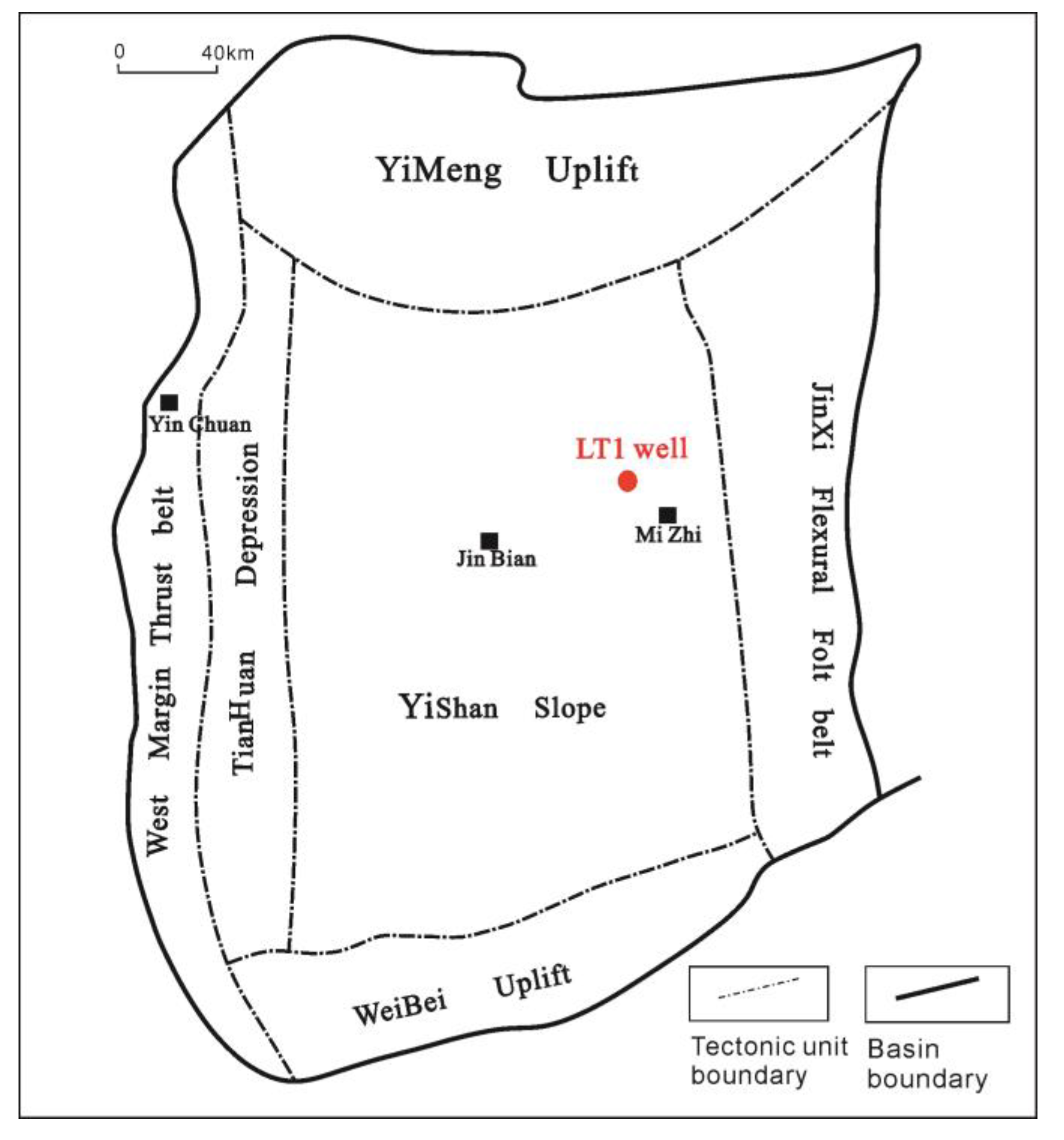
2. Geological Background

The Ordos Basin is the second largest sedimentary basin in China, with a basin area of about 25 × 10⁴ km². This basin is a multicycle sedimentary Craton petroliferous basin with stable sedimentation, migrating depression and obvious torsion. It is a polybasic compound sedimentary basin of Meso–Cenozoic and Proterozoic and Paleozoic rocks [19].

The Ordos Basin has two sets of source rocks, including the Upper Paleozoic marine-continental transitional coal series and Lower Paleozoic marine carbonate rocks. There are sufficient gas sources [20].

The study area is in the LT1 well area in the east of the Ordos Basin (Figure 1).

The target strata in this study are Ma 3 and submembers 6–10 of Ma 5 (Ma 5₆, Ma 5₇, Ma 5₈, Ma 5₉ and Ma 5₁₀) in the Ordovician Majiagou Formation. Major lithologic rocks include dolomite, limestone, salt rock, gypsum rock and mudstone.

Ma 1 and Ma 3 are characteristics of anhydrite centered at salt rocks and evaporation lacustrine deposits of dolomite. The Ma 5₆, Ma 5₈ and Ma 5₁₀ are secondary regressive sediments, which mainly include gypsum-bearing dolomite and gypsum rocks. Ma 5₇ and Ma 5₉ are secondary transgressive deposits, which is mainly composed of carbonate rocks (Figure 2). The Majiagou Formation has mainly experienced three large-scale changes in sea level from the M1 to M6. The sea level dropped and part of the water remained on the land during the deposition period of M1, M3 and M5. A large amount of gypsum salt rock was formed by evaporation and concentration. The salinization process makes water anoxic and forms a reducing environment favorable for organic matter preservation. A large amount of organic matter is enriched and high-abundance source rocks can be formed.

3. Data Preparation

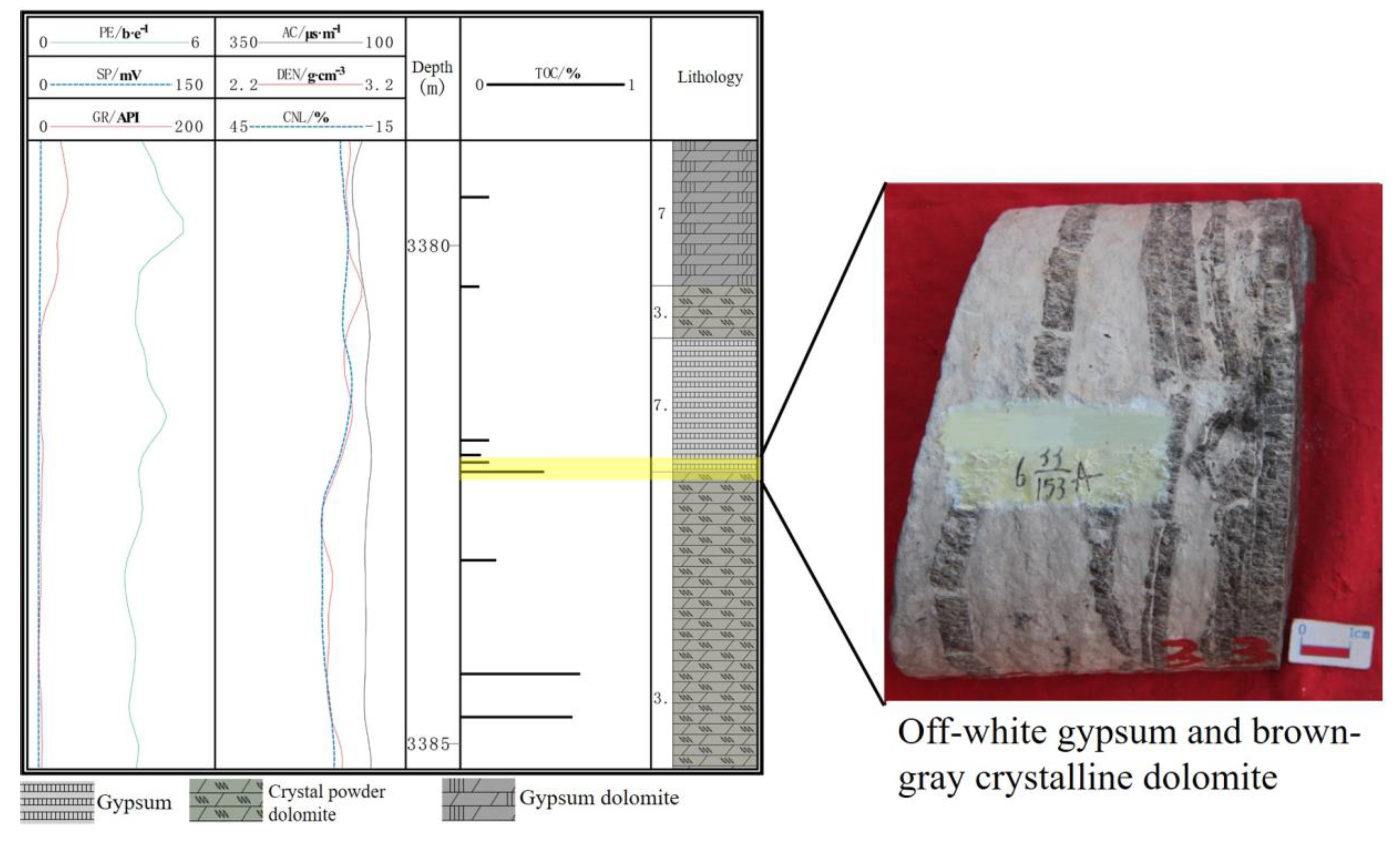
3.1. Optimal Sampling

Source rocks in the Majiagou Formation in the Ordos Basin mainly include the thin-layered dark dolomite mudstones and argillaceous dolomite. The LT1 well has full-section coring and plenty of TOC measured data. There are relatively complete conventional logging data, including natural gamma, interval transit time, neutron porosity, density and resistivity. Therefore, the core of LT1 well in the eastern Ordos Basin was chosen and logging data were used as the basic data. After core location and logging normalization, 309 TOC measured data and corresponding logging data were gained.

During the sedimentary period of the Majiagou Formation in the eastern Ordos Basin, sea level changed frequently, thus resulting in the very complicated lithology and common thin interbedded formations. It can be seen from Figure 3 that gypsum rock and dolomite are in thin alternating deposit and thickness of some lithologic strata is smaller than 1 cm, lower than the logging resolution. Although core lithology changes, the logging curve shows no obvious responses, thus causing mismatching rock–electricity relations. Although there’s relatively high TOC in some thin strata, they are too thin to generate obvious logging responses (Figure 3).

Moreover, TOC logging responses are not significant due to the general inadequate TOC measured data of source rock in the study area. Moreover, external factors (e.g., lithology) influence logging response greatly. As a result, the correlation between TOC measured data and logging data is very poor (Figure 4). It is necessary to process TOC sample data.

To assure consistency of resolution between core data and logging data and increase the correlation between TOC measured data and corresponding logging data, the laboratory TOC measured data were processed by observing the following of two principles.

1. For the section with relatively homogenous lithology, actual core lithology and the mean TOC was used.

2. For the section with thin complicated lithology, and due to a thin stratum being difficult to be used as an effective source rock (although there’s a very high TOC content), the core lithology in this section was used to represent the lithology and TOC of this section was the mean after exclusion of singular values.

Based on above principles, 158 sample points were chosen as the sample data to construct the TOC quantitative log interpretation model.

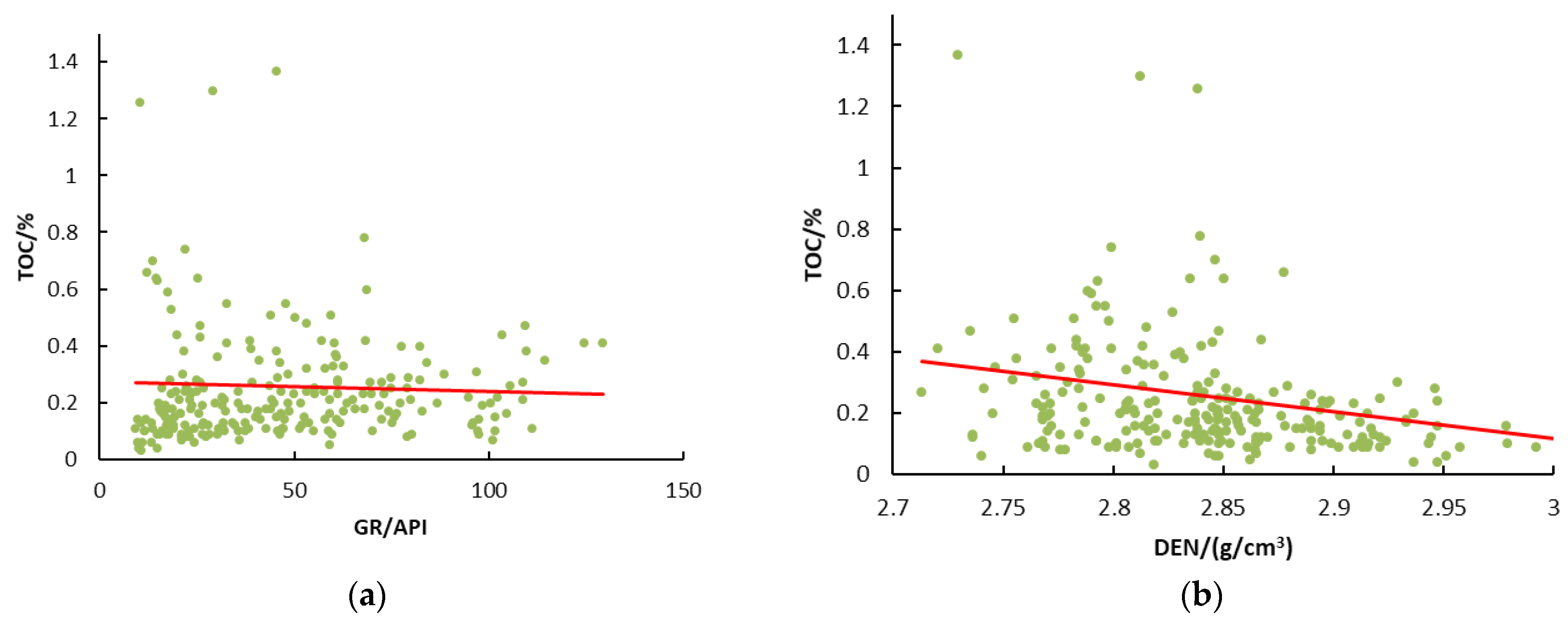
3.2. Correlation Analysis of Logging Curves

Correlation analysis result is an important basis for the TOC quantitative prediction model to select logging data. Through correlation analysis, logging data that are highly related with TOC sample data were chosen to establish the TOC quantitative prediction model. The most sensitive logging parameters to TOC changes were determined according to the correlation analysis between 158 TOC measured samples and logging data (Figure 5).

Radioactivity of source rocks mainly comes from clay minerals and organic carbon. In the deposition process, radioactive elements are adsorbed by clay minerals and organic matters, thus increasing the radioactivity of source rocks. The reducing environment which is formed by kerogen in source rock is beneficial for sedimentation of the radioactive element Uranium (U). In addition, source rock is characteristic of fine particles and a large surface area. Organic matters in source rock have strong absorptivity of radioactive elements [21,22]. Hence, organic content influences the numerical value of natural gamma-ray logging. The radioactivity of source rock is strengthened with the increase of TOC content. The TOC content is positively related with natural gamma (Figure 5a).

Organic matters in source rock belong to a medium to high interval transit time. The interval transit time increases due to the existence of organic matters. TOC content is positively related with interval transit time (Figure 5b).

Solid organic matters are lighter than protolith and their density is close to that of water [23]. Moreover, the density of source rock is negatively related with maturity. With the increase of organic content, density of source rocks decreases (Figure 5c).

Macerals of organic matters in source rock are rich of element hydrogen, which influence the neutron logging value and bring abnormal high values of neutron logging. Therefore, neutron porosity is positively related with TOC content (Figure 5d).

Since kerogen and oil gas have relatively poor conductivity, the formation resistivity increases when there’s organic enrichment. In practical data, resistivity is influenced by TOC slightly due to the low TOC of source rock in the study area. This implies the insignificant correlation between resistivity and TOC (Figure 5e).

Radioactivity in source rock is mainly attributed to radioactive elements (e.g., U), which were adsorbed in the process of sedimentation. Hence, natural gamma spectrometry is positively related with TOC content (Figure 5f–h).

The correlations between re-selected TOC sample data and logging curves are improved significantly. At the 99% confidence level, the T critical value is 2.3578, and the T statistic value of each log data is greater than it (

Table 1. Correlation analysis and significance test of each logging data.

	GR	AC	DEN	CNL	RT	TH	K	U
T	8.9300	5.8818	8.5079	6.5592	3.9892	7.7918	7.9166	4.8520
R	0.5509	0.4144	0.5344	0.4484	0.3059	0.5058	0.5101	0.3579
R2	0.3035	0.1717	0.2856	0.2011	0.0936	0.2548	0.2602	0.1281

), which proves that the variables are significantly correlated at the 99% confidence level. According to correlation analysis, natural gamma spectrometry (K), natural gamma-ray (GR) and density (DEN) are more correlated with TOC.

4. Methods and Results

In this experiment, TOC was predicted by using 158 groups of measured data and corresponding logging data. The traditional ΔlogR method and neural network method were compared and optimized in M3 and M5_6–10 layers. On this basis, it determines that the complicated lithologic TOC interpretation in the study area is applicable to the linear model or nonlinear model. Calculation results were evaluated by the determination coefficient (R²), mean absolute error (MAE), mean relative error (MRE) and root-mean-square error (RMSE). The calculation effect is better if R² approaches to 1 and MAE, MRE and RMSE approach to 0.

4.1. ΔlogR Method

4.1.1. Traditional ΔlogR Method

The TOC calculation formulas of source rock based on the traditional ΔlogR method are the empirical formulas proposed by Passey et al. (Equations (1)–(3)). After combination, the complete TOC calculation formula of traditional ΔlogR method is:

$$\mathrm{TOC}=\lg \left(\mathrm{R}/R_{base}\right)+K·\left(\mathsf{\Delta }\mathrm{t}-\mathsf{\Delta }{t}_{base}\right)·{10}^{2.297-0.1688\mathrm{LOM}}$$

(4)

where R_base and Δt_base are baseline values of resistivity and interval transit time. K is a proportionality coefficient and LOM is maturity of organic matters.

Baseline values are extremely subjective since they have to be determined manually. In addition, it is very difficult to calculate maturity accurately. Therefore, the traditional ΔlogR method has several disadvantages. Moreover, some parameters in the traditional ΔlogR method were gained by Passey et al. according to practical experiences [5]. The traditional ΔlogR method is only applicable to formations with interval transit time of 260~460 μs/m [24]. However, the interval transit time of practical formations in this study area was 130~220 μs/m. Therefore, the formula of traditional ΔlogR method is not applicable to the study area.

4.1.2. Improved ΔlogR Method

For source rocks in the same formation in practical working areas, R_base and Δt_base in the traditional ΔlogR formula (Equation (4)) can be viewed as constant; maturity of source rocks is basically consistent. The coefficient K can be gained through fitting of practical data; therefore, the original TOC formula can be simplified into:

TOC = a·lgR + b·Δt + c

(5)

where a, b and c can be gained through fitting of practical data of working areas.

Sample data were brought into Equation (5) for parameter fitting using SPSS software. The TOC log interpretation formulas corresponding to different target formations are gained.

Ma 5: TOC = 0.323 − 0.107 LgR + 0.0089 Δt

(6)

Ma 3: TOC = −0.268 − 0.071 LgR + 0.0043 Δt

(7)

where R is the value of resistivity curve and Δt is the value of interval transit time.

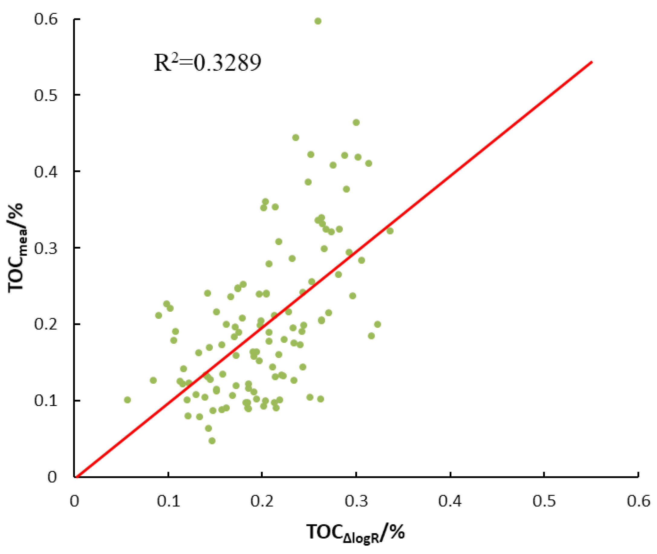
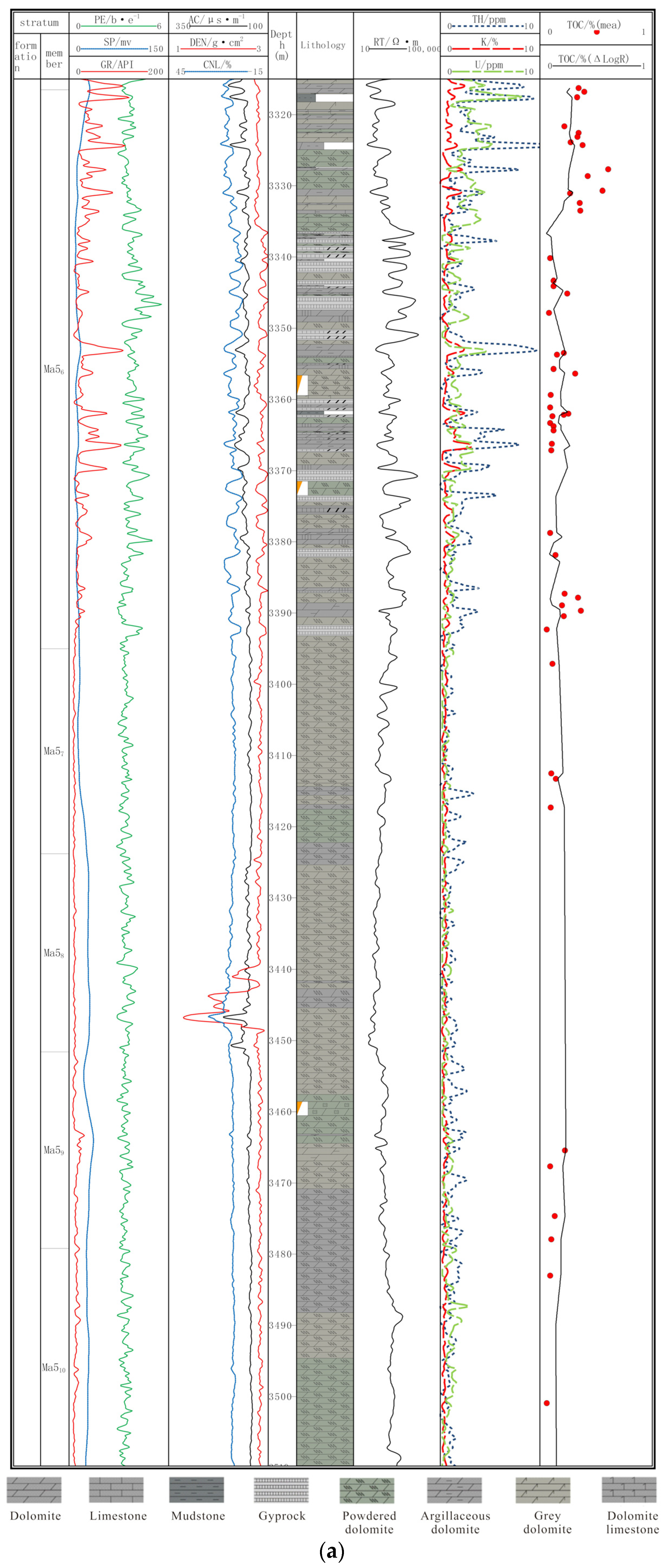
4.1.3. Interpretation Effect Analysis of the ΔlogR Method

Scatter plot of predicted TOC and measured TOC was gained from the prediction model (Figure 6). Meanwhile, the R², MAE, MRE and RMSE were calculated 0.3289, 0.0671, 33.02% and 8.406%, respectively.

The TOC of LT1 well was interpreted by the ΔlogR method and the linear relationship between interpreted TOC and measured TOC was poor (Figure 6). Furthermore, interpretation results were input into the software and a continuous TOC curve was plotted. It found that the curve could not match well with the laboratory measured TOC of core and it could only reflect the general variation trend (Figure 7).

4.2. Neural Network Method

4.2.1. Basic Principle

The BP (back propagation) neural network decreases the error between the output data and sample results by correcting weights of internal layers of existing learning samples, finally getting a relatively perfect neural network. This network is mainly composed of three parts (Figure 8). Part 1 is responsible for inputting original data for the next training; this part is called the input layer. Part 2 is the core of neural network, which is responsible for processing of input data and analyzing characteristics of data. However, specific operation of this process is kept within the network and this part is called the hidden layer. Part 3 is responsible for outputting data processed by the previous part and is called the output layer. In every part of the neural network, each layer is composed of several neural nodes and they are connected mutually into the neural network.

The training process of the BP neural network is a transmission process of data among different neural nodes. After data input, data firstly transmits from the input layer to the output layer, during which each layer is endowed with certain weights. After the processed input data arrive at the output layer, they will be compared with the expected data and differences are calculated. If the error is in the preset permissible range, data can be output. At this moment, neural network training is finished. If error exceeds the permissible range, the error propagates from the input layer to the output layer, during which weights of each layer are modified continuously. After finishing the correction, the processed data are compared with the expected data again and their error is calculated. This process repeats until the error reaches the permissible range.

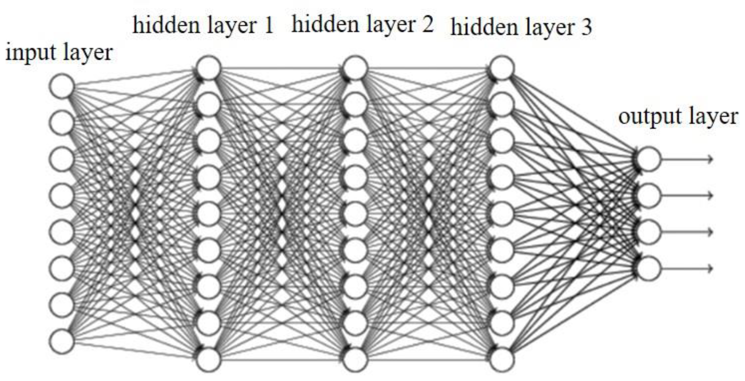
4.2.2. Construction of Neural Network

A BP neural network was built using the MATLAB software. A large sample size can assure that the neural network learns data features to the maximum extent and thus increases accuracy of the neural network. To construct the BP neural network, it usually needs data processing, data input, parameter setting and algorithm selection. The whole process is introduced as follows:

1. Data normalization

Since different logging data have different units that may influence training of the model, it is necessary to implement normalization of TOC data and logging data before the logging data are input into the model in order to improve accuracy of the model and shorten operation time. The normalization uses the range method and its formula is:

$$X_n=\frac{X-X_{min}}{X_{max}-X_{min}}$$

(8)

where X_n is the sample normalization result of logging curve, X is the original logging value, X_min is the minimum and X_max is the maximum.

2. Data input

According to correlation analysis results, the normalized K, GR and DEN logging data were input into the neural network.

To avoid overfitting and assure training quality, a cross-training verification mode was used in the training process of the neural network. Training set, verification set and test set were allocated randomly according to proportions of 70%, 15% and 15%, respectively. Data in the training set (110 groups) were used for the neural network to learn and identify data characteristics. Data in the verification set (24 groups) were used to test whether overfitting occurs (if the error between data used for learning that are output by the neural network and real results decreases, but the error between the current data group after neural network output and the real result is unchanged, overfitting occurs). Data in the test set (24 groups) were used to test unknown sample prediction capacity of the neural network.

3. Parameter setting of the hidden layer

Increasing hidden layers can decrease the error of the neural network and increase the interpretation accuracy. Nevertheless, excessive hidden layers may cause more operations during data transmission in the neural network, so it takes more time for assignment of each layer. Moreover, increasing hidden layers is conducive to explore data characteristics more carefully. With limitations of sample size, some characteristics might exist in learning samples only and they are not applicable to whole data. Hence, overfitting occurs. The BP neural network still can approach any function by adjusting training times or number of nodes in the hidden layer even though it contains only one hidden layer. To decrease calculation while assuring accuracy of the neural network, the number of hidden layers was set 1 during construction of the BP neural network.

Setting the number of nodes in the hidden layer is crucial to construction of the neural network. If the number of nodes is too high, it increases computational loads during data transmission in the neural network. If the number of nodes is too low, it is impossible to learn data features accurately so that the trained neural network cannot recognize the unlearned samples. To determine number of nodes in the hidden layer, several studies have been carried out and many empirical formulas have been proposed.

According to the Kolmogorov theorem, when there’s only one hidden layer, the number of nodes meets:

N_hid = 2N_in + 1

(9)

where N_hid is the number of nodes in the hidden layer and N_in is the number of nodes in the input layer.

The number of nodes in the hidden layer, proposed by Jadid et al. [25], meets:

N_hid ≤ N_train/R × (N_in + N_out)

(10)

where N_train is number of training samples and N_out is number of nodes in the output layer, 5 ≤ R ≤ 10.

Different scholars use different methods to calculate number of nodes in the hidden layer. There’s no uniform formula to calculate the number of nodes in the hidden layer. The distribution range of the number of nodes in the hidden layer is usually calculated according to the empirical formula and then verifies and determines a specific number according to practical data. To optimize the neural network structure and save the learning time of characteristics, it is suggested to use the least nodes while assuring precision. Based on the above formula, the number of nodes in the hidden layer of the neural network shall be 3~13. The neural network was trained with data of practical working areas. When there were 9 nodes in the hidden layer, the training error was the lowest and the correlation among samples was the maximum (

Table 2. The MSE and correlation of different node quantities in the hide layer.

Number of Nodes	3	4	5	6	7	8	9	10	11	12	13
Error/10−3	9.13	8.62	8.44	6.52	6.89	5.75	5.26	5.82	6.14	5.97	6.25
Correlation/10−1	7.27	7.26	7.34	8.51	7.45	9.01	9.39	8.82	9.16	8.78	8.24

). Therefore, the number of nodes in the hidden layer of the constructed neural network was determined to be 9 in this study area.

4. Algorithm selection

The Levenberg–Marquardt algorithm, Bayesian regularization algorithm and quantitative conjugate gradient algorithm are three common algorithms during data training [26].

The Levenberg–Marquardt algorithm is characteristic of quick calculation, but it incurs a operation machine requirement. The Bayesian regularization algorithm avoids overfitting of a characteristic variable by retaining all characteristic variable, which takes a longer operation time. The quantitative conjugate gradient algorithm doesn’t need linear searching, has quick operation and requires a small computational memory, but is not applicable to all datasets. According to practical verification, the Levenberg–Marquardt algorithm can complete neural network training the most quickly and accurately; this algorithm was chosen for data training for the neural network in this study.

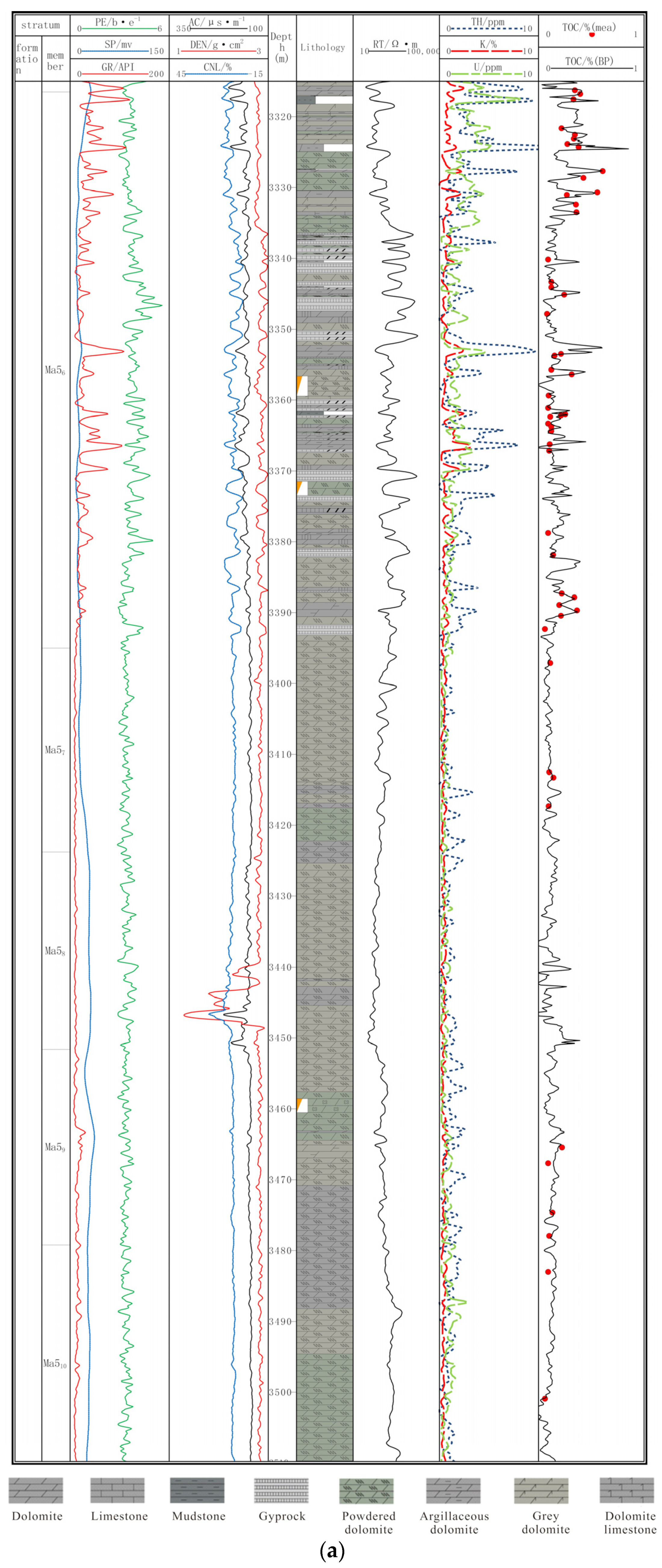
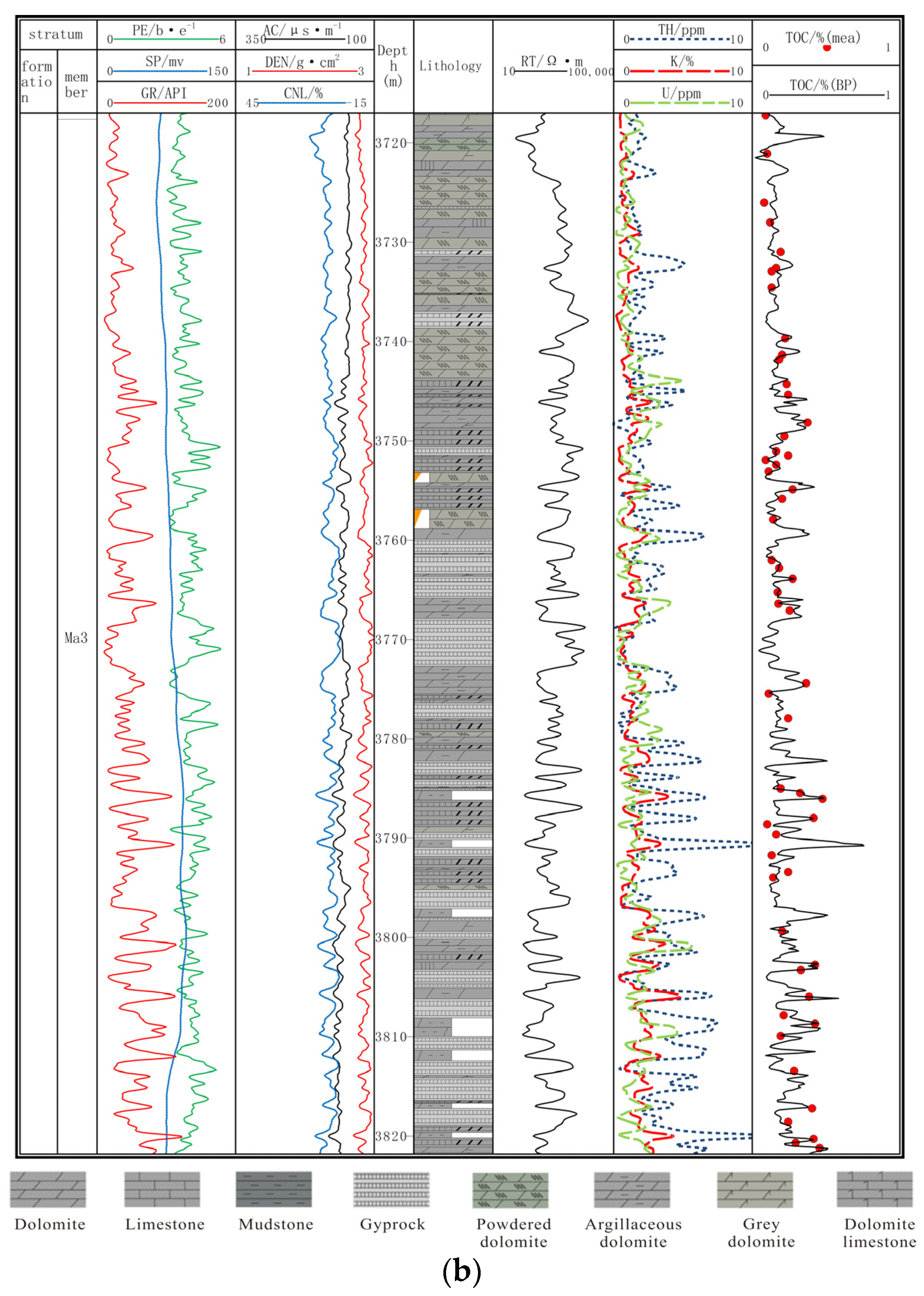
4.2.3. Interpretation Effect Analysis of Neural Network Method

The scatter plot between predicted TOC and measured TOC was gained according to output results of the neural network (Figure 9). Meanwhile, the R², MAE, MRE and RMSE were calculated 0.8254, 0.0322, 15.88% and 4.297%, respectively.

Interpretation results were input into the software and a continuous TOC curve was plotted (Figure 10). Clearly, the fitting degree between the predicted TOC and measured TOC is high, indicating the relatively good prediction effects.

5. Discussion

The predicted parameters of the ΔLogR method and the neural network method are summarized in

Table 3. Summary table of evaluation parameters.

	R2	MAE	MRE	RMSE
ΔLogR method	0.33	0.0671	33.02%	8.41%
Neural network method	0.83	0.0322	15.88%	4.30%

.

Calculated results of the ΔlogR model and neural network model were compared (Table 3). R² of the neural network model is closer to 1 and RMSE is closer to 0 compared to those of the ΔlogR model, indicating that calculated results of the neural network are closer to measured TOC. Moreover, the neural network shows the better TOC calculation efficiency in the level of mathematical indexes. According to practical calculation effects of TOC (Figure 11), the neural network model is more applicable to accurate calculation of TOC in the background of quick changing lithology. On the contrary, the ΔlogR model can only reflect the overall variation trend of TOC, but cannot depict detailed changes of TOC.

The ΔlogR method used only two kinds of logging information during identification of source rocks. However, GR logging and DEN logging also can reflect information of source rock, which are not used in the ΔlogR method. This might be one of the reasons for the poor application effects of the ΔlogR method in the study area. According to previous analysis of correlation between the measured TOC and logging curves, it also found that the correlation between TOC of source rocks and resistivity in the study area is extremely small with almost no correlations. This might be another reason of poor application effects of the ΔlogR method in the study area. The ΔlogR method usually has good application effects in regions with stable lithology. In the study area, there’s complicated and quick changing lithology, which also leads to the poor application effect of the ΔlogR method in this study area.

According to research results in this study, neural network is significantly superior to the traditional ΔlogR method in terms of TOC calculation effect in regions with complicated and changing lithology. The predicted TOC distribution of neural network is closer to practical geological conditions. The neural network method has important significance to further petroleum exploration and development in the future.

6. Conclusions

In this study, the neural network in the AI field was introduced into the TOC logging calculation. The traditional ΔlogR method and neural network method were used for TOC log interpretations of source rock, which has low abundance and complicated lithology in the Majiagou Formation in the LT1 well of the eastern Ordos Basin. Some major conclusions could be drawn:

1. There’s low abundance of source rock in the study area and logging response to TOC is not significant. The complicated and changing lithology also weakens influences of TOC variations on logging, thus resulting in the generally poor correlations between logging data and measured TOC. Therefore, the ΔlogR method, which calculates TOC based on linear relationship is difficult to get the ideal outcomes. The calculated results of ΔlogR method can only reflect the general longitudinal variation trend of TOC but cannot provide a thorough depiction of TOC changes.

2. When calculating TOC in lithologic alternating regions, the neural network model can retain details of TOC changes and thereby reflect TOC changes truly. Furthermore, the neural network model has higher prediction accuracy and stronger adaptation due to the remarkable nonlinear mapping capacity and flexible network structure. It can provide more real references for petroleum exploration and development in the future.

References

1. Schmokerj, W. Determination of Organic-Matter Content of Appalachian Devonian Shales from Gamma-Ray Logs. AAPG Bull. 1981, 65, 1285–1298. [Google Scholar]
2. Chen, Z.; Hao, S.; Xi, S. Logging Evaluation Method for Organic Matter Abundance of Carbonate Source Rock. J. Univ. Pet. (Ed. Nat. Sci.) 1994, 18, 16–19. [Google Scholar]
3. Xu, S.; Zhu, Y. Well logs response and prediction model of organic carbon content in source rocks—a case study from the source rock of Wenchang formation in the pearl mouth basin. Pet. Geol. Exp. 2010, 32, 290. [Google Scholar]
4. Du, W.; Wang, P.; Liang, M. Well logs response characteristics and quantitative prediction model of organic carbon content of hydrocarbon source rocks in coal-bearing strata measures. J. China Coal Soc. 2016, 41, 954–963. [Google Scholar]
5. Passey, Q.R.; Creaney, S.; Kulla, J.B.; Stroud, J.D. A Practical Model for Organic Richness from Porosity and Resistivity Logs. AAPG Bull. 1990, 74, 1777–1794. [Google Scholar]
6. Yu, H.; Rezaee, R.; Wang, Z.; Han, T.; Zhang, Y.; Arif, M.; Johnson, L. A new method for TOC estimation in tight shale gas reservoirs. Int. J. Coal Geol. 2017, 179, 269–277. [Google Scholar] [CrossRef] [Green Version]
7. Yan, J.; Cai, J.; Zhao, M.H.; Zheng, D.S. Advances in the study of source rock evaluation by geophysical logging and its significance in resource assessment. Prog. Geophys. 2009, 24, 270–279. [Google Scholar]
8. Meng, Z.; Guo, Y.; Liu, W. Relationship between organic carbon content of shale gas reservoir and logging parameters and its prediction model. J. China Coal Soc. 2015, 40, 247–253. [Google Scholar]
9. Tan, M.; Bai, Y.; Wang, Q.; Wu, J.; Shi, Y.J.; Li, G.R.; Wei, X.P. Proceedings of the 2019 Oil and Gas Geophysics Annual Conference; Oil and Gas Geophysics Professional Committee of the Chinese Geophysical Society: Nanjing, China, 2019. [Google Scholar]
10. Alizadeh, B.; Najjari, S.; Kadkhodaie-Ilkhchi, A. Artificial neural network modeling and cluster analysis for organic facies and burial history estimation using well log data: A case study of the South Pars Gas Field, Persian Gulf, Iran. Comput. Geosci. 2012, 45, 261–269. [Google Scholar] [CrossRef]
11. Bakhtiar, H.A.; Telmadarreie, A.; Shayesteh, M.; Fard, M.H.H.; Talebi, H.; Shirband, Z. Estimating Total Organic Carbon Content and Source Rock Evaluation, Applying ΔlogR and Neural Network Methods: Ahwaz and Marun Oilfields, SW of Iran. Liq. Fuels Technol. 2011, 29, 1691–1704. [Google Scholar] [CrossRef]
12. Li, Z.; Du, W.; Hu, J.; Li, D. Prediction of shale organic carbon content support vector machine based on logging parameters. Coal Sci. Technol. 2019, 47, 199–204. [Google Scholar]
13. Rui, J.; Zhang, H.; Zhang, D.; Han, F.; Guo, Q. Total organic carbon content prediction based on support-vector-regression machine with particle swarm optimization. J. Pet. Sci. Eng. 2019, 180, 699–706. [Google Scholar] [CrossRef]
14. Amosu, A.; Imsalem, M.; Sun, Y. Effective machine learning identification of TOC-rich zones in the Eagle Ford Shale. J. Appl. Geophys. 2021, 188, 104–113. [Google Scholar] [CrossRef]
15. Liu, X.; Lei, Y.; Luo, X.; Wang, X.; Chen, K.; Cheng, M.; Yin, J. TOC determination of Zhangjiatan shale of Yanchang formation, Ordos Basin, China, using support vector regression and well logs. Earth Sci. Inform. 2021, 14, 22–34. [Google Scholar] [CrossRef]
16. Zhao, W.; Gao, H.; Yan, G.; Guo, T. TOC prediction technology based on optimal estimation and Bayesian statistics. Lithol. Reserv. 2020, 32, 86–93. [Google Scholar]
17. Yin, M.; Cen, C.; Ruan, J.; He, W.W. Classification and prediction method of total organic carbon content in shale gas reservoir based on Bayesian discrimination. J. Geol. 2020, 44, 362–369. [Google Scholar]
18. Rui, J.; Zhang, H.; Ren, Q.; Yan, L.; Guo, Q.; Zhang, D. TOC content prediction based on a combined Gaussian process regression model. Mar. Pet. Geol. 2020, 118, 104–118. [Google Scholar] [CrossRef]
19. Li, G.; Zhao, T.; Shi, Y.; Hu, C.; Chen, Z.; Fan, X.; Li, D.; Lai, J. Diagenetic facies logging recognition and evaluation of carbonate reservoirs in Majiagou Formation, Ordos Basin. Acta Pet. Sin. 2018, 39, 1141–1154. [Google Scholar]
20. Guo, Y.; Zhao, Z.; Zhang, Y.; Xu, W.; Bao, H.; Zhang, Y.; Gao, J.; Song, W. Development characteristics and new exploration areas of marine source rock in Ordos Basin. Acta Pet. Sin. 2016, 37, 939–951. [Google Scholar]
21. Qin, J.Q.; Fu, D.L.; Qian, Y.F.; Yang, F.; Tian, T. Progress of geophysical methods for the evaluation of TOC of source rock. Geophys. Prospect. Pet. 2018, 57, 803–812. [Google Scholar]
22. Dong, H.C. Application of natural gamma spectroscopy logging. Petrochem. Ind. Technol. 2017, 24, 260. [Google Scholar]
23. Zhong, W.J.; Li, H.; Ge, Z.W.; Dong, X.X. Optimum method for calculating organic carbon content from logging data—Taking Longmaxi Formation Shale in X area of southern Sichuan as an example. China Pet. Chem. Stand. Qual. 2020, 40, 12–14. [Google Scholar]
24. Bian, L.; Liu, G.; Sun, M.; Yang, D.; Wan, W.; Zhang, Y. Improved ΔlogR technique and its application to predicting total organic carbon of source rocks with middle and deep burial depth. Pet. Geol. Recovery Effic. 2018, 25, 40–45. [Google Scholar]
25. Jadid, M.N.; Fairbairn, D.R. The application of neural network techniques to structural analysis by implementing an adaptive finite-element mesh generation. AI EDAM 1994, 8, 177–191. [Google Scholar] [CrossRef]
26. Chen, M. Analysis and Compare of BP Neural Network’s Training Arithmetic. Sci. Technol. Plaza 2010, 23, 24–27. [Google Scholar]
Figure 1. Location map of the study area.
Applsci 11 08724 g001
Figure 2. Formation histogram of Majiagou Formation in the eastern Ordos Basin.
Applsci 11 08724 g002
Figure 3. Schematic diagram of core logging.
Applsci 11 08724 g003
Figure 4. Scatter plot of intersection between original TOC data and some logging data: (a) natural gamma ray and (b) organic matter density.
Applsci 11 08724 g004
Figure 5. Correlation between TOC content and (a) natural gamma ray, (b) acoustic time difference, (c) organic matter density, (d) neutron porosity, (e) formation resistivity, (f) uranium, (g) kalium and (h) thorium.
Applsci 11 08724 g005aApplsci 11 08724 g005b
Figure 6. Scatter plot of predicted TOC and measured TOC by ΔLogR method.
Applsci 11 08724 g006
Figure 7. TOC prediction results by Δlog R method in LT1 well: (a) Ma 56–10 and (b) Ma 3.
Applsci 11 08724 g007aApplsci 11 08724 g007b
Figure 8. Neural network structure.
Applsci 11 08724 g008
Figure 9. Scatter plot of predicted TOC and measured TOC by neural network.
Applsci 11 08724 g009
Figure 10. TOC prediction of LT1 well based on the neural network method: (a) Ma 56–10 and (b) Ma 3.
Applsci 11 08724 g010aApplsci 11 08724 g010b
Figure 11. TOC calculation results of different models in well LT1.
Applsci 11 08724 g011