Abstract
Society’s energy consumption has shot up in recent years, making the prediction of its demand a current challenge to ensure an efficient and responsible use. Artificial intelligence techniques have proven to be potential tools in handling tedious tasks and making sense of large-scale data to make better business decisions in different areas of knowledge. In this article, the use of random forests algorithms in a Big Data environment is proposed for household energy demand forecasting. The predictions are based on the use of information from different sources, confirming a fundamental role of socioeconomic data in consumer’s behaviours. On the other hand, the use of Big Data architectures is proposed to perform horizontal and vertical scaling of the solution to be used in real environments. Finally, a tool for high-resolution predictions with great efficiency is introduced, which enables energy management in a very accurate way.
1. Introduction
In recent years, population increase, together with the demands of comfort and the emergence of new technological devices, have been reflected in a rapid intensification in energy consumption. This amount to 39% and of total energy demand and 38% and of carbon dioxide () emissions in the United States and Europe, respectively [1]. That is why forecasting of energy demands in residential buildings is necessary to maximize energy planing, management and resources conservation [2].
Digital progress has also been redesigned in the electrical system through the so-called Smart Grid, which are emerging with the purpose of achieving a more reliable, efficient, safe and sustainable electricity supply, with greater interaction by the consumer [3,4]. This intelligent system allows data exchange between electricity distribution companies, new service providers and users, by combining information and communication technologies with automation and control, through a more flexible distributed network structure [5]. In addition, cloud computing systems, mobile platforms and sensors of various kinds have made it possible to carry out large scale data analysis and offer real time information, including smart electricity meters to control energy flow [5,6]. This knowledge related to the energy behavior of users has a double advantage: it offers greater flexibility, business control and personalized marketing strategies to producers and suppliers, while users can adjust and optimize their consumption and reduce costs.
The large amounts of data generated by these systems have large storage and analysis requirements. Big Data architectures allows to solve this issue through parallel computing, either in cloud systems or distributed computing. These complex architectures provide powerful tools for companies data storage and management, including high availability (data available at all times), scalability (adjustable resources to ingestion and processing processes), redundancy (to prevent data loss) and partitioning (to increase system performance).
These Big Data technologies are combined with artificial intelligence approaches, to maximize knowledge provided by huge amount of data collected, with the purpose of gaining a deeper understanding of household energy consumption and foretell customer’s future behaviours. In this regard, the most recent studies related to energy consumption using Machine Learning and artificial intelligence, Amasyali and El-Gohary [1] found a lack of studies related to residential buildings (only a ) which besides had low precision (only used “sub-hourly” data). Chen et al. [7] found the highest spatio-temporal resolution when using daily data (cumulative daily consumption and average temperature), although the increase of data spatial resolution improved accuracy. In addition, they reviewed the resolution and type of 24 models recently applied to explain the temperature vs. energy consumption, finding 12 applying linear regression, 4 using non-linear regression, and three employing mixed models. From them, only 9 used hourly and one sub-hourly data (which included resolutions at device level for individual households), while only 1 considered data at “sub-city” level and 9 at city level.
Regarding the methodology used for energy demand forecasting, artificial neural networks (ANNs) are becoming very popular, especially for energy planning [8,9,10,11], although many other nonlinear models simpler than ANNs are being used, including decision trees and Random Forest (RF) [10,12,13,14,15], finding both as viable and accurate alternatives Tso and Yau [16]. For instance, Yu et al. [15] developed a model for energy demand prediction in 80 Japanese buildings using a decision tree with an accuracy of for training data and for test data.
With reference to variables governing household energy consumption, climate is one of the most important, although prediction still remains a challenge due to the variety of additional factors that affect, such as the diverse nature of the residential sector, physical properties of the building, installed equipment, energy prices, demographic and socioeconomic factors [17,18], and the type of energy used [7,19,20,21,22]. Furthermore, spatio-temporal variations in electricity consumption is higher compared to other sectors (such as commercial or industry), which adds uncertainty in the prediction [23,24].
The proposal of this paper is to combine meteorological and socioeconomical data with the power of available energy smart meters from The Low Carbon London (LCL) trial project [25] to address the challenge of predicting energy consumption in households, using the tools provided by artificial intelligence in a distributed environment.
Two studies have already analysed these data with two different approaches. Mingyang Sun et al. [17] used a metric widely used in the UK’ planning guidelines called after-diversity maximum demand (ADMD), which determines coincident peak energy demand for a large number of customers [26,27,28]. Their findings were based on ACORN classification using only 2013 data, and considering the number of household occupants as additional variable to determine general household demands for distribution planning practices. In this study, the importance of socioeconomic factors in energy demand is confirmed, as the need of further studies taking into consideration calendar seasons, days and hours, as the work in this paper.
On the other hand, Dong et al. [18] studied the accuracy and computational times of RF for hourly energy prediction using Apache Spark in AWS S3 as scalable distributed storage infrastructure and MongoDB as database. They confirmed, as it has been done in this paper, the need of a distributed architecture to improve computational times and predictive accuracy for large-scale datasets.
With the evidence of the precious studies in analyzing demands at different levels of resolutions and the proposal of Big Data technologies for large-scale datasets, the novelty of this paper lies in the use of artificial intelligence approaches to analysis data with high temporal resolution (hourly), including socioeconomic variables that allow to break up the data-set in groups, increasing resolution of the results. Finally, the use of non-linear models allows more flexibility in contrast to the stiffness of mostly used linear models [16,29].
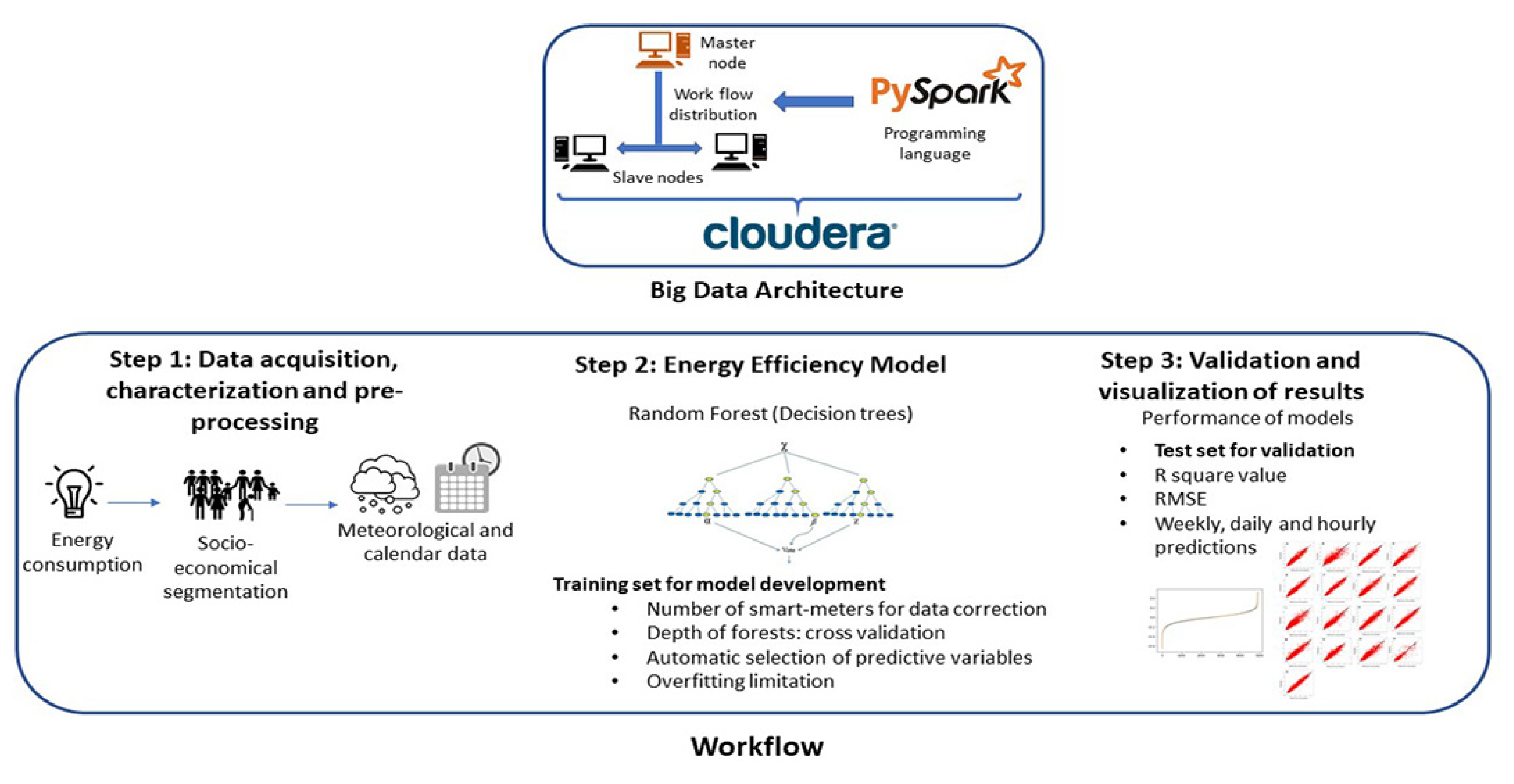
To ensure the scalability and availability of the generated solution for a real application with larger data flows, a Spark distributed Cluster allocated in Cloudera platform is presented as the big data architecture for the querying and data processing, using the native Machine Learning module of Spark (MLlib).
2. Methodology
This section includes a description of the proposed methodology, summarized in the graphical abstract of Figure 1. It is divided in three steps summarizing the main workflow, which will be further developed in the next subsections. The first step, data acquisition, characterization and preprocessing, consists of collection of household energy consumption data and associated variables, including socio-economical factors for clients categorization and meteorological and calendar information to characterize the energy demands. Step 2, energy efficiency model, covers the process for developing the prediction models based on decision trees and the data collected in Step 1. Finally, Step 3, validation and visualization of results, comprises the statistical variables applied to determine models performance and their comparison with existing studies using the same data. Besides, the architecture in which the previous steps are deployed is explained in Section 2.4.

Figure 1.
Main workflow proposed: Data acquisition and preprocessing, Energy eddiciency model and Validation of results.
2.1. Step 1: Data Acquisition, Characterization and Preprocessing
Development of a consistent prediction model includes four main steps as part of a Knowledge Data Discovery (KDD) process: data acquisition, preprocessing, model training and validation.
Regarding data acquisition, home electricity consumption for 4404 households with fix tariffs (not subject to dynamic time of use) were acquired from the Low Carbon London project led by UK Power Networks [25]. The dataset includes smart meter readings (Landis y Gyr (L + G) E470) taken at half hourly intervals for a period between November 2011 and February 2014. All selected households depended solely on electricity, excluding those with gas, prepaid consumption, micro-generation and in vulnerable situations [30].
The customers in the trial were recruited as a balanced sample representative of the Greater London population, based on their CACI Acorn group [31]. Acorn is a segmentation tool that categorizes UK population in 17 groups (A to Q from higher to lower social status) based on post code and demographic variables (life stiles, behaviours and other socio-economic variables obtained from public and private sources) and statistical algorithms, created to help the public and private sector to develop business strategies.
The meteorological data were collected at hourly basis from a local weather station through website Dark-Sky [32], including the following parameters: temperature (°C); dew point (°C); humidity (0–1 decimal percentage); UV index; wind speed (mph); type of precipitation (rain or snow) and summary of the weather in text format (partially/mostly cloudy/cloudy, foggy, windy, clear, and all possible combinations).
Finally, school calendar, bank holidays, time of day and day type, variables commonly used for their relation to occupancy [33,34,35], were also considered to enhance the performance in the predictions. Furthermore, as the number of costumers during the study is not constant, either because of problems with the smart meters functioning or their staggered entry in the project, an additional variable related to the number of active smart meters was included to correct the predictions.
Data preprocessing consisted of a simple transformation of text and calendar variables into categorical classes to fit into the models and a pre-selection of the attributes based on their co-correlation, because the selected models, explained in the following subsection, have no need for elimination of outliers or additional data transformation [36]. Half hourly energy consumption data were grouped to hourly level to meet meteorological registers. Data rejection and transformation has been kept to minimal to provide the models with the most information possible, but number of active smart-meters was introduced as additional variable to diminish the potential bias associated to the number of connected clients at each moment.
2.2. Step 2: Energy Efficiency Model
An approach based on Random Forest (RF) algorithm was used for predictions. This machine learning algorithm, based on the combination of decision trees, consists of obtaining a segmentation of data by empirical means, applying a consecutive series of simple rules (tree). RF does not require excessive computational capacity while it is able to fit complex nonlinear relationships [12,16,36].
RF, developed by Breiman [37], has been highly successfully applied in general problems both as a regression and classification method, being versatile enough to be applied to problems Large scale and easily adapt to various ad hoc learning tasks [38]. This approach combines several random decision trees using perturbation and combination techniques [39] that consist of creating a set of diverse classifiers introducing randomness in the process of construction of said classifiers. The prediction of the considered set is obtained by using the average prediction of the individual classifiers [40].
In this study, the dataset was firstly tested as a whole and in a second experiment split into 18 groups based on the socioeconomical variables, the ACORN categories, as it was understood that they behave differently.
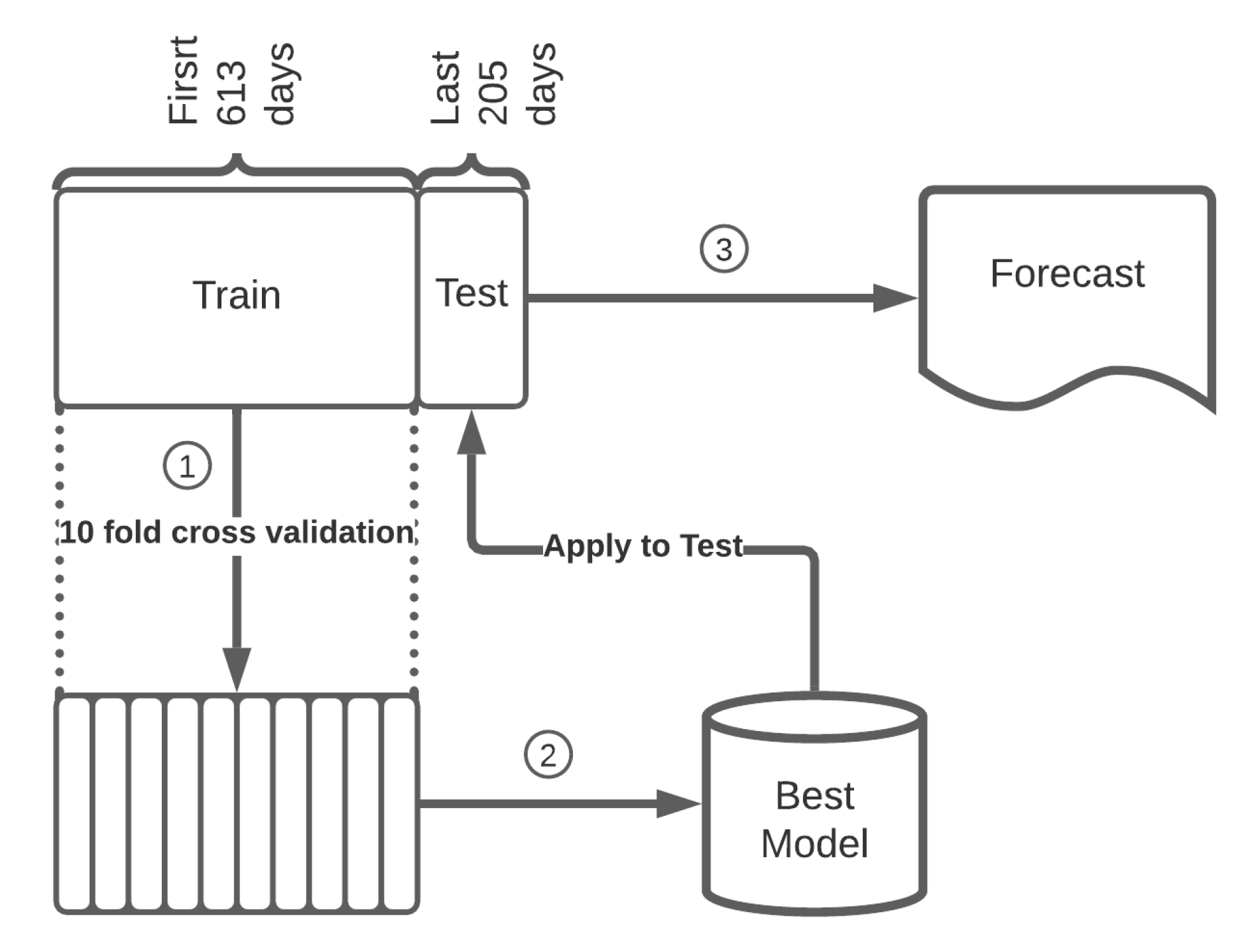
The available data were divided in a 75:25 test:training ratio based on energy sequential observations for each ACORN group (see top left boxes in Figure 2). Thus, the first 613 days of a total of 818 observations of each group were considered for training and the last 205 days for testing. This selection gives a better approximation for a real application, forecasting the energy demand in the next N days after a giving date and under certain conditions, allowing the study of possible deviations that the forecast could suffer over time and the implications this could have in the range of algorithms applicability.

Figure 2.
Diagram of Random Forest empirical model development. Firstly, the training set is used to find the best Random Forest model, applying a cross-validation technique to ensure the optimal maximum depth of trees. Finally, the performance of the forecast is checked using the testing set.
In RF, the more trees assembled, the greater the precision and accuracy, although the results cease to improve significantly beyond a critical number of trees, causing over-fitting. To prevent this phenomenon and ensure the optimal maximum depth of trees, a cross-validation technique was implemented before modeling (see phase number 1 in Figure 2 for more detail), using the training set, 10 random folds and 20, 22, 24, 26, 28 and 30 depths, the maximum number of trees in Spark. With respect to the prediction parameters, the models themselves are able to select the most appropriate ones based on their correlation strength with the explanatory variable and avoid those autocorrelated.
2.3. Step 3: Validation and Visualization of Results
The accuracy of RF trained models was determined using the testing set (more detailed in phases 2 and 3 of Figure 2). This technique is used to ensure that the predictions obtained through the data mining process are independent of the partition between training and test data, was also implemented. Statistical indicators used to evaluate the prediction performance of the models: mean square error (RMSE), coefficient of determination () and normal quantile-quantile (Q-Q) plot. is the most common statistical coefficient used to explain the percentage of the total variance explained by the model [41]. RMSE indicates the variation between the actual and predicted values, and has been widely used as a standard statistical measure of model performance in several fields [42,43,44], being more appropriated than mean absolute error (MAE) when errors follow a normal distribution [45]. A Q-Q plot is a commonly used graphical method to compare empirical and theoretical values of the same model (residuals). This graph provides a fast visualization of trends within the data distribution and can be used to limit the data ranges for which the model can be applied based on residuals deviations [46,47].
2.4. System Recommendation. Big Data Architecture
In terms of computational capacity needed to deploy the machine learning analysis of this study, it was firstly evaluated the number of models and combinations of trees and folds for the cross-validation. In total, 18 models were performed, one for each ACORN group and the combined one for the entire data set. For each of them, six different maximum depths of trees were tested and a 10-fold cross-validation was made to ensure the result. This means 1140 Random Forest Algorithms using a dataset with 167 million rows.
To ensure sufficient computational capacity for this analysis and meet the requirements for a real application in an energy production company [48], a Hadoop Big Data cluster in Cloudera [49,50] was deployed including four nodes of 24 GB each. Apache Spark [51,52] was considered as a good candidate for analytics engine as it offers high data analysis and processing speed capabilities, additional tools and libraries for Machine learning, is designed to easily scale horizontally and can be deployed in numerous Big Data architectures. Besides, Spark allows parallel computing in vertical and horizontal directions, dividing the processes needed for running the multiple Random Forest algorithms in different nodes, including the execution of each algorithm itself, thought map-reduce process. This is a clear advantage for the subsequent application of the results in a real environment with thousands of users connected to the network and sending continuous information. That advantage is used to spread a parallel algorithm for all the cluster but the distributed process has a higher overload to communicate all the results across the network.
In this experiment, the entire dataset was loaded in the cluster and transformed to work in parallel as a Resilient Distributed Dataset (RDD) [53], the basic data type of Spark. The partial results were saved in The Hadoop Distributed File System Mackey et al. [54] (HDFS) while the different algorithms are executed. A PySpark [55] program using Python was executed continuously for two weeks. SparkML [56] was the package chosen to for machine learning algorithms pipelines across the cluster nodes. The optimal depth of trees was explored using a 10-fold cross-validation for each ACORN in a four thread pool, to take full advantage of the cluster’s power. Once this depth was determined, the dataset was divided for training/test.
3. Results and Discussion
The objective of this section is to demonstrate the benefits of our approach in terms of short term predictions, daily and especially hourly level, which provides very high level of detail of what is happening. To do that, we first study the overall group of customers to evidence the need of desegregation in groups of customers to improve predictions. Once the data set is divided by ACORN classification, each group is analyzed to understand what is happening behind the predictions and estimate if RF is able to model hourly behaviour without loosing precision. The raw data used for the predictions, together with the results revised in this section are available at the following repository: https://doi.org/10.5281/zenodo.5483899.
3.1. Importance of Socioeconomic Classification (ACORN)
Table 1 summarizes the performance achieved for each model following the premised from the previous paragraph.

Table 1.
Summary of Random Forest models performance for each Acorn group and ALL data without previous classification.
The row under the name ALL corresponds to the accumulated forecast for the studied population as a whole while the other ones correspond to each ACORN group. Moderate performance is obtained for model ALL attending to , although the value of RMSE is the highest in the table, indicating the model is not able to predict accurately the energy demand of certain part of the population. Therefore, the classification in ACORN groups is seen as an appropriate technique to better cover the consumers’ behaviour. Regarding values for these ACORN models, those with more than of variance explained are ACORN C, H and N. Most ACORN groups have acceptable results around (ACORN A, D, F, G, I, K, L, M, O, P and Q). This technique is not successful for groups E and especially J, with very low values, although they do not have the highest errors based on RMSE. Attending to this last parameter, the lowest errors < 10) are registered for Acorns U, B, C, I, M, N and O while ACORN E has the highest one (110). The other groups register intermediate RMSE values, around 1–30.
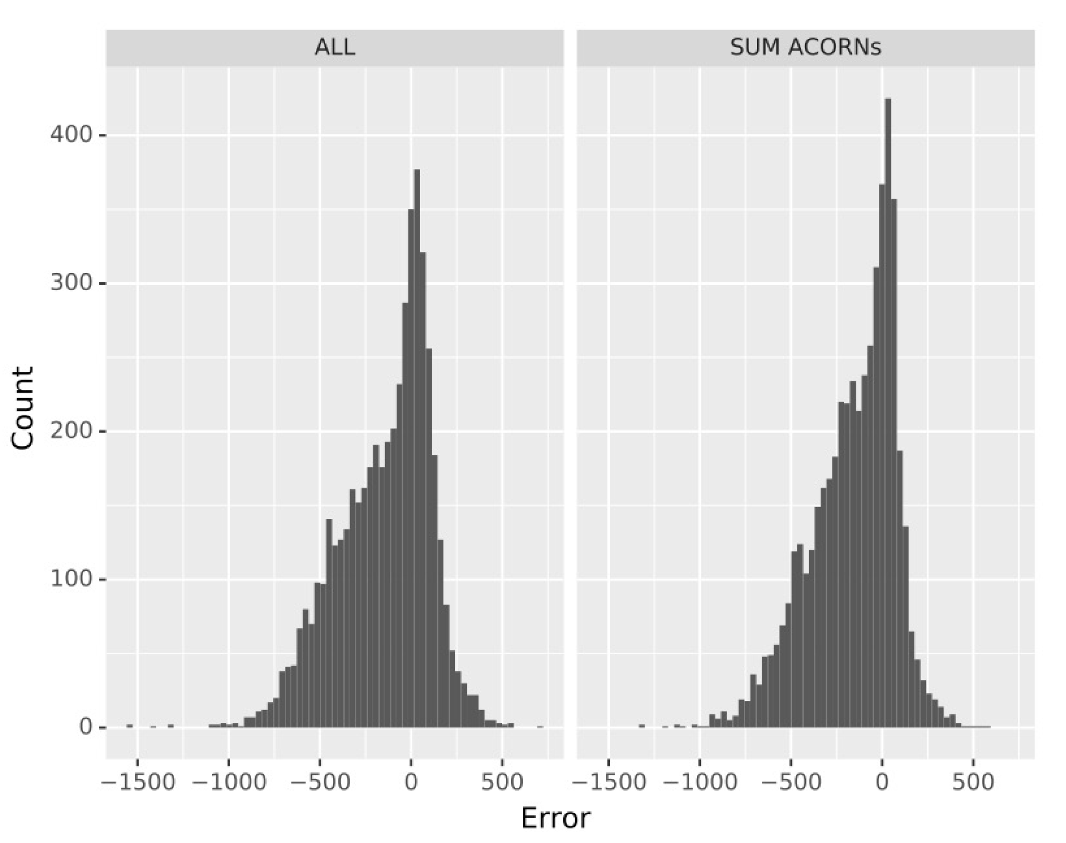
For deeper exploration of results, RF prediction residuals are represented in Figure 3. It was expected that the more grouped the data (ALL), the better the results, as uncertainties and outliers are masked and the common trend stands out. However, the errors in ALL are remarkable, especially in the tails and show a clear bias, which reflects the customers behave differently and a unique model is not suitable for covering the proposed objectives. Therefore, the hypothesis of dividing the customers in groups according to their socioeconomic characteristics (ACORN classes) appears as a wise alternative to reduce uncertainty.
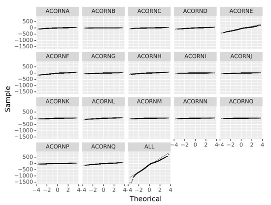
Figure 3.
Residuals q-q Plot for each ACORN group and all the customers (ALL).
When divided by ACORNs, the previous bias disappears and only a slight deviation is detected for most groups, the previous bias disappears, residuals are random and follow a normal distribution and only a slight deviation for extreme data is detected. Therefore, only these grouped data are considered for further analysis.
This becomes clearer when comparing the histogram of the residuals for all the customers and the one for the sum of the residuals of each Figure 4 (ACORN), this last histogram being sharper and with higher values than the first one, indicating the errors are closer to zero. Furthermore, a Kolmogorov–Smirnov non-parametric test of the residuals has been peformed, as the data do not follow a normal distribution, rejecting the null hypothesis and thus confirming the distribution of errors is different in both forecasts.

Figure 4.
Histogram of the residuals for all customers (ALL, left) and the sum of the residuals of each ACORN individually (right).
3.2. Energy Demand Forecasts
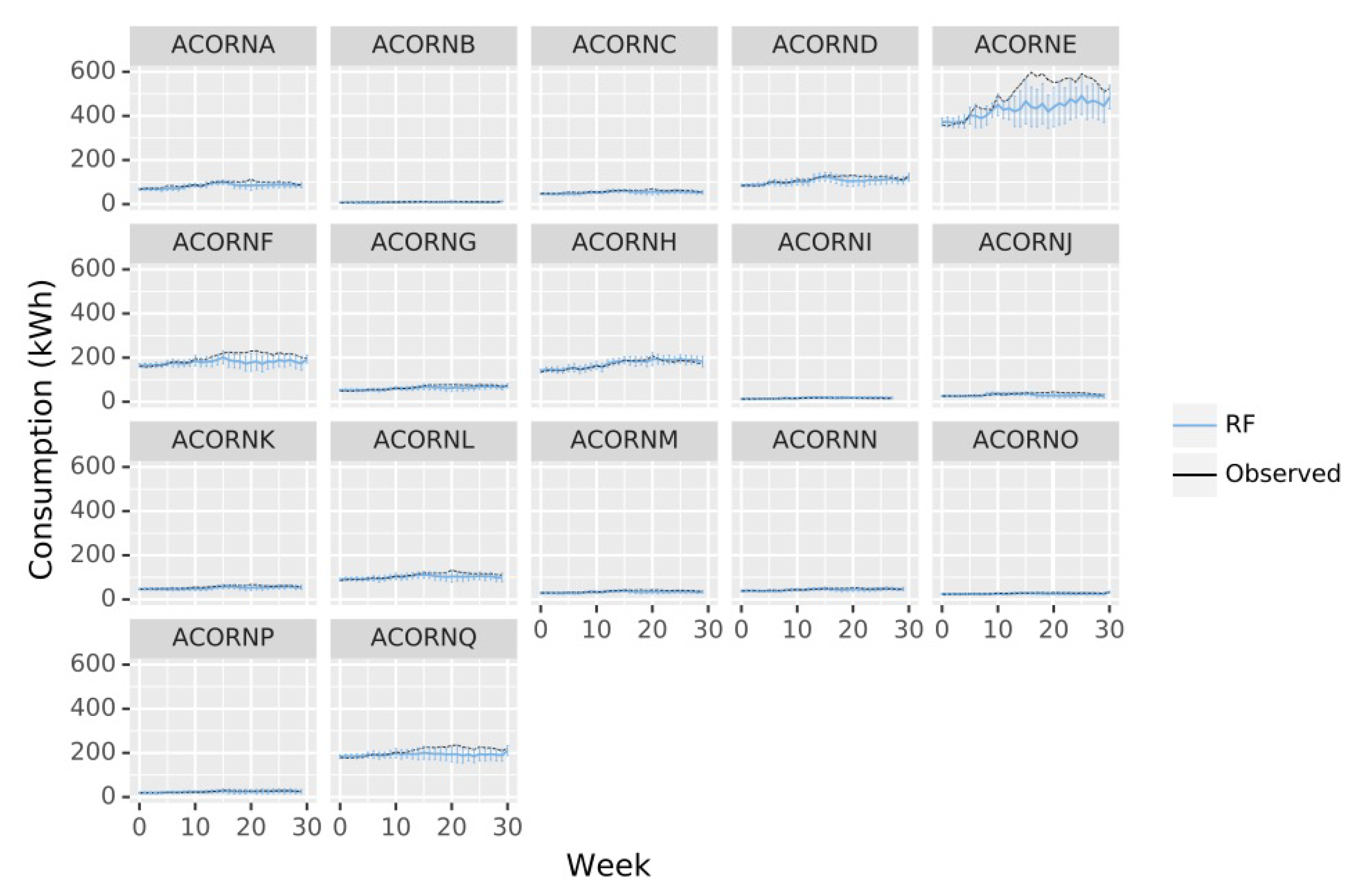
Once the evidence of including socioeconomic variables to improve energy demand predictions is retrieved, three different approaches were considered: weekly, daily and hourly forecasts (Figure 5, Figure 6 and Figure 7).
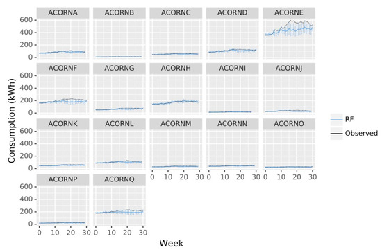
Figure 5.
Energy consumption observations (kWh, black line) across the latest 270 days of data against RF mean predictions by week of the year (average 24 h and 7 days observations) for each ACORN group (blue line). Represented observed data are average values. Error bars represent predictions square deviation of the 24 h and 7 days average observations.
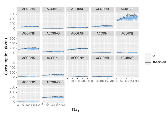
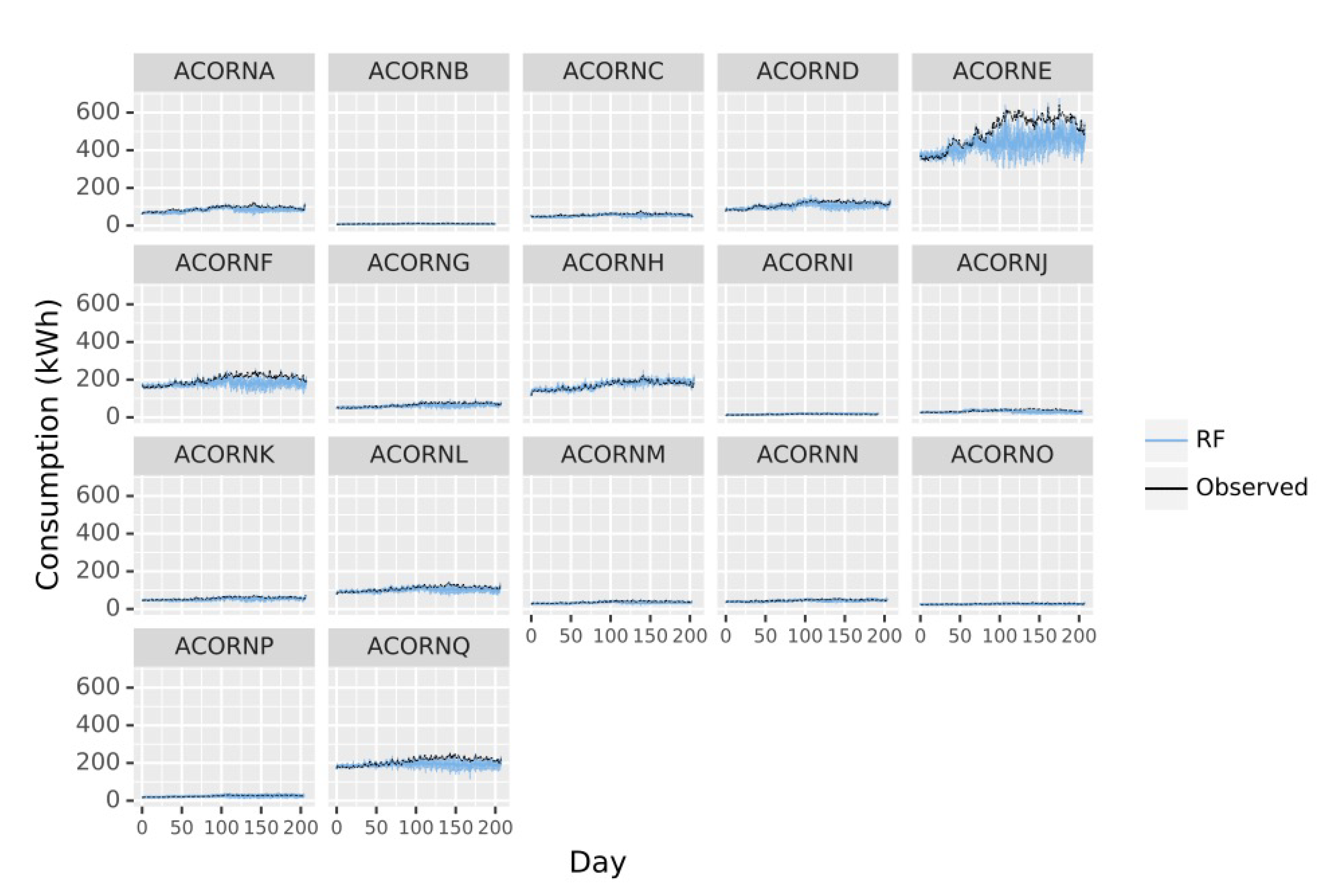
Figure 6.
RF mean predictions by day of the week (average values of 24 h observations) for each ACORN group across the latest 270 days of data. Error bars represent predictions square deviation considering average 24 h errors.

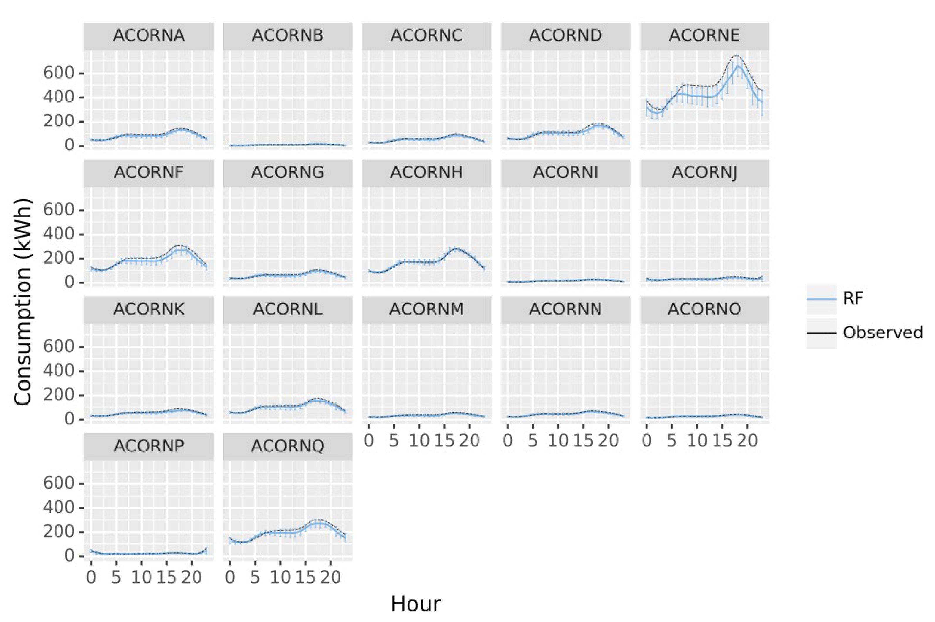
Figure 7.
RF mean predictions by hour of the day for each ACORN group across the latest 270 days of data. Error bars represent predictions square deviation.
Considering the errors made in weekly predictions, it is especially significant how the errors are very low for the first five weeks but they start increasing from then to the week number ten, when there is no only an error increment but also a remarkable deviation between the prediction and the real value, indicating the temporal limit of the algorithms applicability. For both weekly and daily predictions, ACORN E presents very high deviations from observation, which indicates the model does not perform well. ACORN F also suffers a slight deviation, especially for the intermediate period during validation, while the other groups are very adjusted to expected values. ACORN E and F are also the ones with higher demands, which could indicate that the groups of high social status do not have the highest needs as their households are more energetically sustainable, there are additional variables not considered in this study that could be influencing consumption for middle class population.
Hourly forecasts follow a different pattern to the previous predictions for all groups, with a clear variation of consumption along the day, emphasizing daily predictions miss important information for short term applications. In general terms, errors rise during the evening (15.00–20.00) coinciding with the hours of maximum energy demand, due to a more variable behaviour not covered by the meteorological or general socioeconomic variables studied. Nevertheless, the errors remain low for all groups but again ACORN E, emphasizing the need of more information to characterize this group. Heterogeneity of members of ACORN E must be affecting the prediction, which is defined as “Career Climbers”; young people, single couples, and families with young children who own mortgages on apartments, flats, or small houses, living normally in urban locations. It is surprising that in general, energy demand for ACORN E is higher than groups A or B, with higher socioeconomic status, but considering the model uncertainties and the residuals bias, this group must be not well characterized and a deeper analysis should be made to detect undetected subgroups.
4. Conclusions
In this article, Big Data technologies are proposed to predict energy demands in the household. Specifically, the machine learning algorithm Random Forest is run in a horizontal and vertical scaling architecture at different levels of resolution (weekly, daily and hourly forecast), which allows to get the most out of the system in real environments with high detail level.
To analyze the potential of our proposal, the importance of customer’s socioeconomic information is analyzed in the first place. In this sense, it is evidenced that even the quality of the results without using these variables is acceptable in absolute error terms, it is not able of capturing the behaviours of certain customers with demands far from the mean. Thus, the usefulness of ACORN socioeconomic segmentation is accepted to refine the results.
On the other side, the behaviour of the proposal is studied attending to different levels of resolution, weekly, daily and hourly, showing that Random Forest is able to make predictions at very high level of resolution without losing quality in the results and very similar errors. In addition, with this approach it is possible to detect variations in the energy demands resulting from variables not covered by meteorological or socioeconomic data. Likewise, it is evident that the prediction at different resolutions is very close to the real behaviour when the time elapsed between the value to be predicted and the last one recorded is short. However, the error increases with higher differences in time between the prediction and the last observation, which shows a time limit in the application of this kind of algorithm.
With reference to the architecture, a Hadoop Big Data cluster in Cloudera was deployed. Four nodes were needed for the used data load although it is designed to scale vertical and horizontally to improve analysis performance to be applied in real environments.
Author Contributions
Conceptualization, J.I.M. and N.D.-D.; Data curation, L.C.; Formal analysis, L.C.; Funding acquisition, N.D.-D.; Methodology, J.I.M.; Software, J.I.M.; Supervision, N.D.-D.; Validation, N.D.-D.; Visualization, J.I.M.; Writing—original draft, L.C.; Writing—review & editing, J.I.M. and N.D.-D. All authors have read and agreed to the published version of the manuscript.
Funding
This research was partially supported by the Ministry of Economy and Competitiveness, project TIN2015-64776-C3-2-R, and by the Junta de Andalucia, under the Andalusian Plan for Research, Development and Innovation, TIC-239.
Institutional Review Board Statement
Not applicable.
Informed Consent Statement
Not applicable.
Data Availability Statement
Conflicts of Interest
The authors declare no conflict of interest.
References
- Amasyali, K.; El-Gohary, N.M. A review of data-driven building energy consumption prediction studies. Renew. Sustain. Energy Rev. 2018, 81, 1192–1205. [Google Scholar] [CrossRef]
- Wang, Z.; Srinivasan, R.S. A review of artificial intelligence based building energy use prediction: Contrasting the capabilities of single and ensemble prediction models. Renew. Sustain. Energy Rev. 2017, 75, 796–808. [Google Scholar] [CrossRef]
- Kragh-Furbo, M.; Walker, G. Electricity as (Big) Data: Metering, spatiotemporal granularity and value. Big Data Soc. 2018, 5, 1–12. [Google Scholar] [CrossRef] [Green Version]
- Huh, J.H.; Otgonchimeg, S.; Seo, K. Advanced metering infrastructure design and test bed experiment using intelligent agents: Focusing on the PLC network base technology for Smart Grid system. J. Supercomput. 2016, 72, 1862–1877. [Google Scholar] [CrossRef]
- Jo, H.; Yoon, Y.I. Intelligent smart home energy efficiency model using artificial TensorFlow engine. Hum.-Centric Comput. Inf. Sci. 2018, 8, 1–18. [Google Scholar] [CrossRef]
- Aman, S.; Simmhan, Y.; Prasanna, V. Energy Management Systems: State of the Art and Emerging Trends. IEEE Commun. Mag. 2013, 51, 114–119. [Google Scholar] [CrossRef]
- Chen, M.; Ban-Weiss, G.A.; Sanders, K.T. The role of household level electricity data in improving estimates of the impacts of climate on building electricity use. Energy Build. 2018, 180, 146–158. [Google Scholar] [CrossRef]
- Ahmad, T.; Chen, H.; Shah, W.A. Effective bulk energy consumption control and management for power utilities using artificial intelligence techniques under conventional and renewable energy resources. Int. J. Electr. Power Energy Syst. 2019, 109, 242–258. [Google Scholar] [CrossRef]
- Debnath, K.B.; Mourshed, M. Forecasting methods in energy planning models. Renew. Sustain. Energy Rev. 2018, 88, 297–325. [Google Scholar] [CrossRef] [Green Version]
- Ahmad, M.W.; Mourshed, M.; Rezgui, Y. Trees vs. Neurons: Comparison between random forest and ANN for high-resolution prediction of building energy consumption. Energy Build. 2017, 147, 77–89. [Google Scholar] [CrossRef]
- Ahmad, M.W.; Mourshed, M.; Yuce, B.; Rezgui, Y. Computational intelligence techniques for HVAC systems: A review. Build. Simul. 2016, 9, 359–398. [Google Scholar] [CrossRef] [Green Version]
- Genuer, R.; Poggi, J.M.; Tuleau-Malot, C.; Villa-Vialaneix, N. Random Forests for Big Data. Big Data Res. 2017, 9, 28–46. [Google Scholar] [CrossRef]
- Ibarra-Berastegi, G.; Saénz, J.; Esnaola, G.; Ezcurra, A.; Ulazia, A. Short-term forecasting of the wave energy flux: Analogues, random forests, and physics-based models. Ocean. Eng. 2015, 104, 530–539. [Google Scholar] [CrossRef]
- Lahouar, A.; Slama, J.B.H. Day-ahead load forecast using random forest and expert input selection. Energy Convers. Manag. 2015, 103, 1040–1051. [Google Scholar] [CrossRef]
- Yu, Z.; Haghighat, F.; Fung, B.C.; Yoshino, H. A decision tree method for building energy demand modeling. Energy Build. 2010, 42, 1637–1646. [Google Scholar] [CrossRef] [Green Version]
- Tso, G.K.; Yau, K.K. Predicting electricity energy consumption: A comparison of regression analysis, decision tree and neural networks. Energy 2007, 32, 1761–1768. [Google Scholar] [CrossRef]
- Sun, M.; Konstantelos, I.; Strbac, G. Analysis of diversified residential demand in London using smart meter and demographic data. In Proceedings of the 2016 IEEE Power and Energy Society General Meeting (PESGM), Boston, MA, USA, 17–21 July 2016; pp. 1–5. [Google Scholar] [CrossRef]
- Dong, C.; Du, L.; Ji, F.; Song, Z.; Zheng, Y.; Howard, A.; Intrevado, P.; Woodbridge, D.M.; Howard, A.J. Forecasting Smart Meter Energy Usage Using Distributed Systems and Machine Learning. In Proceedings of the 2018 IEEE 20th International Conference on High Performance Computing and Communications, IEEE 16th International Conference on Smart City, IEEE 4th International Conference on Data Science and Systems (HPCC/SmartCity/DSS), Exeter, UK, 28–30 June 2018; pp. 1293–1298. [Google Scholar] [CrossRef]
- Huang, J.; Gurney, K.R. Impact of climate change on U.S. building energy demand: Sensitivity to spatiotemporal scales, balance point temperature, and population distribution. Clim. Chang. 2016, 137, 171–185. [Google Scholar] [CrossRef]
- Kavousian, A.; Rajagopal, R.; Fischer, M. Determinants of residential electricity consumption: Using smart meter data to examine the effect of climate, building characteristics, appliance stock, and occupants’ behavior. Energy 2013, 55, 184–194. [Google Scholar] [CrossRef]
- Psiloglou, B.; Giannakopoulos, C.; Majithia, S.; Petrakis, M. Factors affecting electricity demand in Athens, Greece and London, UK: A comparative assessment. Energy 2009, 34, 1855–1863. [Google Scholar] [CrossRef]
- Lam, J.C. Climatic and economic influences on residential electricity consumption. Energy Convers. Manag. 1998, 39, 623–629. [Google Scholar] [CrossRef]
- Lam, J.C.; Tang, H.; Li, D.H. Seasonal variations in residential and commercial sector electricity consumption in Hong Kong. Energy 2008, 33, 513–523. [Google Scholar] [CrossRef]
- Hirano, Y.; Fujita, T. Evaluation of the impact of the urban heat island on residential and commercial energy consumption in Tokyo. Energy 2012, 37, 371–383. [Google Scholar] [CrossRef]
- UK-Power-Networks. SmartMeter Energy Consumption Data in London Households—London Datastore. 2011. Available online: https://data.london.gov.uk/dataset/smartmeter-energy-use-data-in-london-households (accessed on 27 May 2021).
- McQueen, D.H.O.; Hyland, P.R.; Watson, S.J. Monte Carlo simulation of residential electricity demand for forecasting maximum demand on distribution networks. IEEE Trans. Power Syst. 2004, 19, 1685–1689. [Google Scholar] [CrossRef]
- Barteczko-Hibber, C. After Diversity Maximum Demand (ADMD) Report. In Report for the ‘Customer-Led Network Revolution’ Project; Durham University: Durham, UK, 2015. [Google Scholar]
- Richardson, I.; Thomson, M.; Infield, D.; Clifford, C. Domestic electricity use: A high-resolution energy demand model. Energy Build. 2010, 42, 1878–1887. [Google Scholar] [CrossRef] [Green Version]
- Kuster, C.; Rezgui, Y.; Mourshed, M. Electrical load forecasting models: A critical systematic review. Sustain. Cities Soc. 2017, 35, 257–270. [Google Scholar] [CrossRef]
- Bilton, M.; Carmichael, R.; Dragovic, J.; Schofield, J.; Woolf, M.; Strbac, G. Accessibility and validity of Smart meter data. Report C5 for the Low Carbon London LCNF Project. In Report C5 for the “Low Carbon London” LCNF Project; Imperial College London: London, UK, 2014. [Google Scholar]
- CACI. The Acorn User Guide. The Consumer Classification; CACI: London, UK, 2010. [Google Scholar]
- Dark-Sky. Dark Sky API: Documentation Overview. 2021. Available online: https://darksky.net/dev/docs (accessed on 27 May 2021).
- Leung, M.; Tse, N.C.; Lai, L.; Chow, T. The use of occupancy space electrical power demand in building cooling load prediction. Energy Build. 2012, 55, 151–163. [Google Scholar] [CrossRef]
- Edwards, R.E.; New, J.; Parker, L.E. Predicting future hourly residential electrical consumption: A machine learning case study. Energy Build. 2012, 49, 591–603. [Google Scholar] [CrossRef]
- Escrivá-Escrivá, G.; Álvarez Bel, C.; Roldán-Blay, C.; Alcázar-Ortega, M. New artificial neural network prediction method for electrical consumption forecasting based on building end-uses. Energy Build. 2011, 43, 3112–3119. [Google Scholar] [CrossRef]
- Elith, J.; Leathwick, J.; Hastie, T. A working guide to boosted regression trees. J. Anim. Ecol. 2008, 77, 802–813. [Google Scholar] [CrossRef] [PubMed]
- Breiman, L. Random Forests. Mach. Learn. 2001, 45, 5–32. [Google Scholar] [CrossRef] [Green Version]
- Biau, G.; Scornet, E. A random forest guided tour. Test 2016, 25, 197–227. [Google Scholar] [CrossRef] [Green Version]
- Breriman, L. Arcing classifiers. Ann. Stat. 1998, 26, 801–824. [Google Scholar]
- Garreta, R.; Moncecchi, G. Learning Scikit-Learn: Machine Learning in Python; Packt Publishing Ltd.: Birmingham, UK, 2013. [Google Scholar]
- Cheng, C.L.; Garg, G. Coefficient of determination for multiple measurement error models. J. Multivar. Anal. 2014, 126, 137–152. [Google Scholar] [CrossRef] [Green Version]
- Arthur, E.; Rehman, H.U.; Tuller, M.; Pouladi, N.; Nørgaard, T.; Moldrup, P.; de Jonge, L.W. Estimating Atterberg limits of soils from hygroscopic water content. Geoderma 2021, 381, 114698. [Google Scholar] [CrossRef]
- Liu, D.; Guo, S.; Zou, M.; Chen, C.; Deng, F.; Xie, Z. A dengue fever predicting model based on Baidu search index data and climate data in South China. PLoS ONE 2019, 14, 120. [Google Scholar] [CrossRef] [Green Version]
- McKeen, S.; Wilczak, J.; Grell, G.; Djalalova, I.; Peckham, S.; Hsie, E.; Gong, W.; Bouchet, V.; Menard, S.; Moffet, R.; et al. Assessment of an ensemble of seven realtime ozone forecasts over eastern North America during the summer of 2004. J. Geophys. Res. 2005, 110, D21307. [Google Scholar] [CrossRef]
- Chai, T.; Draxler, R.R. Root mean square error (RMSE) or mean absolute error (MAE)—Arguments against avoiding RMSE in the literature. Geosci. Model Dev. 2014, 7, 1247–1250. [Google Scholar] [CrossRef] [Green Version]
- Borojerdnia, A.; Rozbahani, M.M.; Nazarpour, A.; Ghanavati, N.; Payandeh, K. Application of exploratory and Spatial Data Analysis (SDA), singularity matrix analysis, and fractal models to delineate background of potentially toxic elements: A case study of Ahvaz, SW Iran. Sci. Total Environ. 2020, 740, 140103. [Google Scholar] [CrossRef] [PubMed]
- Aieb, A.; Lefsih, K.; Scarpa, M.; Bonaccorso, B.; Cicero, N.; Mimeche, O.; Madani, K. Statistical modeling of monthly rainfall variability in Soummam watershed of Algeria, between 1967 and 2018. Natural Resour. Model. 2020, 33, e12288. [Google Scholar] [CrossRef]
- Shanmugam, K. Best Practices for Successfully Managing Memory for Apache Spark Applications on Amazon EMR. 2019. Available online: https://aws.amazon.com/es/blogs/big-data/best-practices-for-successfully-managing-memory-for-apache-spark-applications-on-amazon-emr/ (accessed on 5 July 2021).
- Cloudera. Ecosistema de Apache Hadoop. 2021. Available online: https://es.cloudera.com/products/open-source/apache-hadoop.html (accessed on 5 July 2021).
- Shvachko, K.; Kuang, H.; Radia, S.; Chansler, R. The Hadoop Distributed File System. In Proceedings of the 2010 IEEE 26th Symposium on Mass Storage Systems and Technologies (MSST), Incline Village, NV, USA, 3–7 May 2010; pp. 1–10. [Google Scholar] [CrossRef]
- Foundation, T.A.S. ApacheSpark. Lightning-Fast Unified Analytics Engine. 2018. Available online: https://spark.apache.org/ (accessed on 10 July 2021).
- Salloum, S.; Dautov, R.; Chen, X.; Peng, P.X.; Huang, J.Z. Big data analytics on Apache Spark. Int. J. Data Sci. Anal. 2016, 1, 145–164. [Google Scholar] [CrossRef] [Green Version]
- Foundation, T.A.S. RDD Programming Guide. Available online: https://spark.apache.org/docs/latest/rdd-programming-guide.html (accessed on 7 July 2021).
- Mackey, G.; Sehrish, S.; Wang, J. Improving metadata management for small files in HDFS. In Proceedings of the 2009 IEEE International Conference on Cluster Computing and Workshops, New Orleans, LA, USA, 31 August–4 September 2009; pp. 1–4. [Google Scholar] [CrossRef]
- Drabas, T.; Lee, D. Learning PySpark; Packt Publishing: Birmingham, UK, 2017. [Google Scholar]
- Karim, M.; Kaysar, M. Large Scale Machine Learning with Spark; Packt Publishing: Birmingham, UK, 2016. [Google Scholar]

Publisher’s Note: MDPI stays neutral with regard to jurisdictional claims in published maps and institutional affiliations. |
© 2021 by the authors. Licensee MDPI, Basel, Switzerland. This article is an open access article distributed under the terms and conditions of the Creative Commons Attribution (CC BY) license (https://creativecommons.org/licenses/by/4.0/).