Trajectory Tracking with Adaptive Robust Control for Quadrotor

Abstract

This work proposes three robust mechanisms based on the MIT rule and the sliding-mode techniques. These robust mechanisms have to tune the gains of an adaptive Proportional-Derivative controller to steer a quadrotor in a predefined trajectory. The adaptive structure is a model reference adaptive control (MRAC). The robust mechanisms proposed to achieve the control objective (trajectory tracking) are MIT rule, MIT rule with sliding mode (MIT-SM), MIT rule with twisting (MIT-Twisting), and MIT rule with high order sliding mode (MIT-HOSM).

1. Introduction

Unmanned aerial vehicles (UAVs) have a lot of acceptance in the control theory research due to the challenge of getting a stable flight and finding some application to solve some science and engineering problems. Some applications with these unmanned aerial vehicles are: forest fire detection, in civil engineering (topography, analysis structural and others) [1], photogrammetry, and military applications [2], car detection [3] or for landing [4]. We can find different strategies to resolve the trajectory tracking with a quadrotor; for example, ref. [5] was proposed a flight controller with a hierarchical structure designed to control the altitude and the position. The controllers used in [5] are proportional-derivative (PD) and proportional-integral-derivative (PID) with a genetic algorithm method. In [6], a nonlinear system error was proposed for trajectory tracking of a six-degree of freedom quadrotor, and to stabilize the quadrotor attitude a backstepping approach and a nonlinear disturbance observer/sliding mode control approach are used. Likewise, a nonlinear adaptive state feedback technique as presented in [7,8] was applied to an adaptive algorithm for steering a quadrotor in a trajectory with parametric uncertainty. Then, trajectory tracking with a quadrotor is a problem of accuracy in the position, and in [9] a solution based on trajectory planning algorithm with a genetic algorithm (GA) and A${}^{*}$ algorithm is presented. On the other hand, in [10] a novel 3D path planning technique to steer a sinusoidal path for a quadrotor is presented.

Some scientific research, before resolving the problem of trajectory tracking with a quadrotor, first resolves the problem of the disturbances acting in unmanned aerial vehicles such as in [11], where an estimator considers the sliding mode techniques to attenuate the translational disturbance. In [12], an optimal controller in a quadrotor is applied considering external perturbations in the system and a quadrotor linear mathematical model is considered; that is, the control law is working in some quadrotor operating pue with input constraints to avoid the external disturbances and even is demonstrated finite-time convergence. In [13], a backstepping control and integral sliding mode is proposed to eliminate external perturbations. A novel multivariable super-twisting algorithm to avoid the chattering effect generated by the integral sliding mode is presented in [13]. On the other hand, in [14], a robust controller to stabilize a quadrotor is proposed; the control law was based on the proportional-derivative control, and to obtain a better flight performance a disturbance compensation was introduced. The mathematical model that defines the UAV in [14] is rotation in SO(3). It is worth mentioning that in [11,12,13,14,15] do not applying any adaptive controller.

Other authors suggest that adaptable techniques are better to stabilize a quadrotor. For instance, in [16] an adaptive controller applied to attitude tracking is presented for an unmanned aerial vehicle to eliminate the adverse effect of measurement noises. Even in [17], a robust adaptive neural network controller is proposed, and is applied to a quadrotor UAV. This control law is not necessary for the prior information of disturbances to stabilize the quadrotor. Meanwhile, in [18] an adaptive backstepping is presented with an extended state observer applied to a quadrotor to follow and maintain trajectory, even if it is subject to external disturbances. The perturbations in [16,17,18] are considered as a noise in the measurement from the sensors that feedback the control law. On the other hand, Ref [19] presented the adaptive tracking control for a quadrotor in different or multiple operating conditions. These conditions are when the quadrotor deals with system uncertainties or unknown parameters; the control objective is to obtain a uniform update law for the controller parameters based on the Model Reference Adaptive Control (MRAC). Otherwise, MRAC modification in [20] is used to catch possibly dangerous UAVs mid-air using a net carried by two drones. The modification proposed in [20] is adding a compensation with a proportional-derivative-integral action to avoid instability of the system due to abrupt changes in altitude. Besides, a comparative between Proportional-Integral-Derivative and MRAC control for a quadrotor to stabilize the Euler angles roll, pitch, and yaw was analyzed in [21]. On the other hand, in [22] neural networks were employed to design an indirect MRAC to work for any quadrotor system. The neural networks have to learn the system parameters online (during the flight), and the challenge is to keep the quadrotor stable during online learning. In [23], it is shown how to apply the sliding mode control theory, MRAC, and the adaptive sliding mode control to design flight controllers for quadrotors; these proposals are evaluated and compared in numerical simulations. In [24], a study of multivariable output feedback MRAC applied to a quadrotor with parameter uncertainties is presented. The feedback solution requires one-third the number of measurements as full state feedback. In [25], a baseline MRAC controller applied to a quadrotor is shown with parameter changes or uncertainty parameters during the quadrotor flight, and the recursive least squares method is used with a forgetting factor to identify or estimate the unknown parameters. Otherwise, to solve the problem of parametric and nonparametric uncertainties in quadrotors, a decentralized adaptive controller with the methodology of Lyapunov and with an MRAC structure is presented in [26]. The controller is applied to achieve the desired angles (yaw, pitch, roll) and the desired altitude. Even in [27], the MRAC is used to try with the uncertainties, but it involves the adaptive control only in the Euler angles defined by the approximation of the quadrotor dynamics.

Then the general problem is the trajectory tracking with a quadrotor, and this implies, based on the research presented before, that a controller is necessary for attitude, position, and with enough robustness for the quadrotor to achieve the desired trajectory for some applications as mentioned at the beginning of this introduction. Thus, we proposed resolving this problem with a robust mechanism for an adaptive control law to steer a quadrotor UAV in a predefined trajectory by equations to obtain an adequate trajectory and avoid some physics singularity of the system in the position and the quadrotor attitude.

Then, the controller in this work is an adaptive proportional-derivative control, starting from the methodologies MIT rule and sliding modes. The MIT rule is the original approach to model-reference adaptive control; the name is from the Instrumentation Laboratory (now the Draper Laboratory) at MIT [28].

Specifically, the main contribution of this work is the robustness in the design of the adjustment mechanism that has to adjust the adaptive gains. With this, we can obtain better results in time convergence, reduce the oscillations in the steering trajectory, and obtain a stable flight during some applications. Several simulations are presented to show that the adaptive control law with a robust adjustment mechanism is effective. Other contributions of this work are

• The obtention of robust adaptive controller considering a Proportional-Derivative structure.
• Design only two adjustment mechanisms for two gains and achieve the control objective.
• The obtention of a robust adjustment mechanism with the use of the sliding mode theory.
• Achieve the desired trajectory with a reduced aerodynamic model.
• The modification of the MIT rule is different that that presented in [5,6,7,8,9,10,11,12,13,14,15,16,17,18,19,20,21,22,23,24,25,26,27,28].

This work is organized as follows: Section 2 shows the equations that define the dynamical model of the quadrotor; Section 3 presents the equation to obtain the desired trajectory and Section 4 presents the adaptive controller and robust mechanisms design. In Section 4.1, the simulation results and an analysis of the error signals and the efforts of the control inputs are shown. Section 5 presents the discussion of this work. Finally, in the Appendix A the stability proof of the adaptive PD controller is presented.

2. Mathematical Model

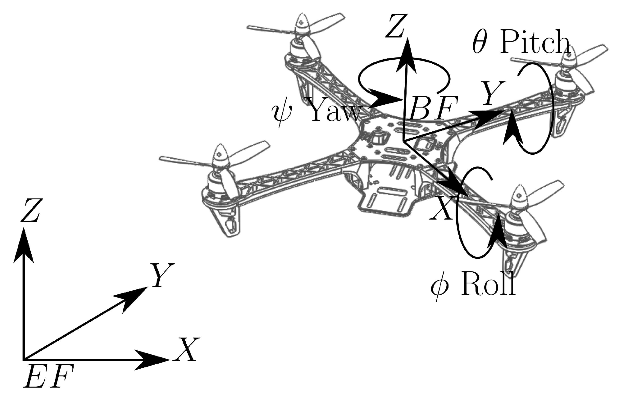
The mathematical model to describe the quadrotor UAV is in three sets of vectors; the first defines the accelerations, the second defines the Euler rates, and the last vector represents the angular accelerations [29]. Then, the accelerations in the body frame (BF) [30] of the unmanned MAV are given by:

$$\overrightarrow{a}=\left(\begin{array}{c}{a}_x\\ a_y\\ a_z\end{array}\right)=\left(\begin{array}{c}gsin\theta \\ -gsin\varphi cos\theta \\ -gcos\varphi cos\theta \end{array}\right)+\left(\begin{array}{c}-2(v_z{w}_y-v_y{w}_z)\\ -2(v_x{w}_z-v_z{w}_x)\\ -2(v_y{w}_x-v_x{w}_y)\end{array}\right)+$$

(1)

$$+\left(\begin{array}{c}2\frac{m_w}{m}(v_y·(w_1+w_2+w_3+w_4))\\ -2\frac{m_w}{m}(v_y·(w_1+w_2+w_3+w_4))\\ 0\end{array}\right)+\left(\begin{array}{c}0\\ 0\\ \frac{1}{m}b(w_1^2+w_2^2+w_3^2+w_4^2)\end{array}\right)$$

(2)

where g is the gravitational constant, $\theta$ is the rotation in the axis-Y, $\psi$ rotation in axis-Z, and $\varphi$ rotation in the axis-X, such rotations correspond to pitch, yaw, and roll, respectively, [29]. The angular velocities are defined as $w_x,w_y,w_z$ and the linear velocity is given by $v_x,v_y,v_z$ about the axis-X, Y and Z, respectively, (see Figure 1). The constant b represents the reaction torque gain coefficient in the Z axis direction, m corresponds to the mass of the vehicle, and $m_w$ is the mass of propellers and rotors is equal to $m_w$.

Thus, the second vector defines the Euler rates; these are used to determine the changes in the quadrotor BF, and local system orientation relative to the auxiliary system is SF:

$$\dot{\overrightarrow{\Theta }}=\left(\begin{array}{c}\dot{\varphi }\\ \dot{\theta }\\ \dot{\psi }\end{array}\right)=\left(\begin{array}{c}{w}_x+w_{y}sin\varphi tan\theta +w_{z}cos\varphi tan\theta \\ w_{y}cos\varphi -w_{z}sin\varphi \\ w_y\frac{sin\varphi }{cos\theta }+w_z\frac{cos\varphi }{cos\theta }\end{array}\right)$$

(3)

The last vector represents the angular accelerations in the unmanned MAV; this vector is given by:

$$\dot{\overrightarrow{\Omega }}=\left(\begin{array}{c}\dot{w_x}\\ \dot{w_y}\\ \dot{w_z}\end{array}\right)=\left(\begin{array}{c}\frac{1}{I_x}l·b(w_4^2-w_2^2)\\ \frac{1}{I_y}l·b(w_3^2-w_1^2)\\ \frac{1}{I_z}d(w_2^2+w_4^2-w_1^2-w_3^2)\end{array}\right)$$

(4)

$$\left(\begin{array}{c}-\frac{1}{I_x}\left(w_y{w}_z(I_z-I_y)\right)\\ -\frac{1}{I_y}\left(w_x{w}_z(I_x-I_z)\right)\\ -\frac{1}{I_z}\left(w_x{w}_y(I_y-I_x)\right)\end{array}\right)\left(\begin{array}{c}-\frac{1}{I_x}\left(w_y{I}_w(w1+w2+w3+w4)\right)\\ -\frac{1}{I_y}\left(w_x{I}_w(w1+w2+w3+w4)\right)\\ 0\end{array}\right)$$

(5)

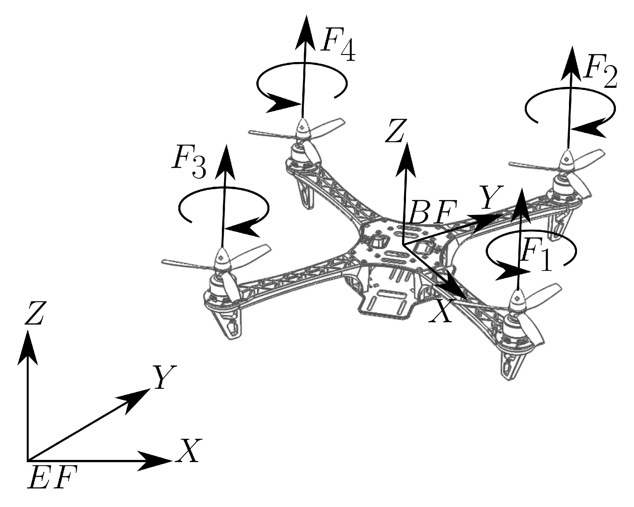
where $I_w$ is the inertia moment in the rotor. $I_x$, $I_y$, and $I_z$ represent the inertia for the x-axis, y-axis, and z-axis, respectively. l is the length of the unmanned aerial vehicle arm [29]. Figure 2 is presented the 4 thrust forces that act in the unmanned aerial vehicle or quadrotor.

Remark 1.

The vector $\overrightarrow{a}$ as well as the vector $\dot{\overrightarrow{\Omega }}$ describe the relationship that exist in the local coordinate system BF. Euler rates vector $\dot{\overrightarrow{\Omega }}$ describes the relationship between systems BF and SF.

3. Trajectory Planner

Before designing the controller is necessary to generate the desired trajectory that must follow the UAV (Unmanned Aerial Vehicle). Then, we have defined a model that represents the acceleration of a particle or solid in the $x-y$ axis given by

$$\begin{array}{ccc}\hfill \ddot{x}& =& g(\theta cos\varphi +\varphi sin\psi )\hfill \end{array}$$

(6)

$$\begin{array}{ccc}\hfill \ddot{y}& =& g(\theta sin\psi -\varphi cos\psi )\hfill \end{array}$$

(7)

Thus, Equations (6) and (7) can be seen as the reference trajectory that the UAV must achieve. To generate the desired trajectory, it is necessary to define two other equations:

$$\begin{array}{ccc}\hfill {\ddot{x}}^c& =& k_{p1}(x_d-x)+k_{d1}({\dot{x}}_d-\dot{x})+{\ddot{x}}_d\hfill \end{array}$$

(8)

$$\begin{array}{ccc}\hfill {\ddot{y}}^c& =& k_{p2}(y_d-y)+k_{d2}({\dot{y}}_d-\dot{y})+{\ddot{y}}_d\hfill \end{array}$$

(9)

with $k_{p1,2},k_{d1,2}>0$. Finally, with Equations (8) and (9), it is possible to obtain the Euler angles that will be the reference inputs for the control law to move the unmanned aerial vehicle toward the desired trajectory. The equations to obtain desired angles are:

$$\begin{array}{ccc}\hfill {\varphi }_c& =& \frac{1}{c}({\ddot{x}}_{c}sin{\psi }^d-{\ddot{y}}_{c}cos{\psi }^d)\hfill \end{array}$$

(10)

$$\begin{array}{ccc}\hfill {\theta }_c& =& \frac{1}{c}({\ddot{x}}_{c}cos{\psi }^d-{\ddot{y}}_{c}sin{\psi }^d)\hfill \end{array}$$

(11)

$$\begin{array}{ccc}\hfill {\psi }_c& =& {\psi }^d\hfill \end{array}$$

(12)

with ${\varphi }_c$ as roll angle reference, ${\theta }_c$ and ${\psi }_c$ are the pitch and yaw angle references, respectively.

4. Adaptive Controller and Robust Mechanisms Design

To achieve the desired trajectory by the quadrotor, we have reduced the mathematical model; this can help demonstrate the effectiveness of the robust mechanisms to achieve the control objective despite the reduced mathematical model. The design of the adjustment mechanisms is with the gradient method used by the MIT rule with sliding mode control theory to give robustness to the adjustment mechanisms. The controller is a PD with adaptive gains, and the critical part of this adaptive law is the adjustment mechanism. Then, the control law is given by

$$u_{\Theta }={\widehat{k}}_{p\Theta }^{al}({\overrightarrow{\Theta }}_c\left(t\right)-\overrightarrow{\Theta }\left(t\right))-{\widehat{k}}_{d\Theta }^{al}({\dot{\overrightarrow{\Theta }}}_c\left(t\right)-\dot{\overrightarrow{\Theta }}\left(t\right))$$

(13)

with ${\overrightarrow{\Theta }}_c\left(t\right)=[{\theta }_c,{\varphi }_c,{\psi }_c]$ and $\overrightarrow{\Theta }\left(t\right)=[\theta ,\varphi ,\psi ]$. Then, $u_{\Theta }=u_{\theta },u_{\varphi },u_{\psi }$ are the adaptive controllers defined to achieve the desired angles and in consequence attain the desired trajectory. The adaptive proportional gain is given as ${\widehat{k}}_{p\Theta }^{al}$ and the adaptive derivative gain is ${\widehat{k}}_{d\Theta }^{al}$. The acronym ”$al$” is used to indicate the adjustment mechanism that schedules the controller gains ($l\in 1,\dots ,4$):

• $a1$: The MIT rule.
• $a2$: The MIT rule with first-order sliding mode (MIT-SM).
• $a3$: The MIT rule with twisting (MIT-Twisting).
• $a4$: The MIT rule with high order sliding mode (MIT-HOSM).

The adaptive controller (13) is applied at a reduced model (pure motion Euler angles) obtained fromf Equations (3) and (4). Then, based on the MIT methodology presented in [28], the mathematical model that represents the unmanned aerial vehicle and the adaptive law is defined in a close-loop transfer function and is given by

$$\overrightarrow{\Theta }\left(t\right)=\frac{({\widehat{k}}_{p\Theta }^{al}+{\widehat{k}}_{d\Theta }^{al}s)C_2}{s^2+(C_2{\widehat{k}}_{d\Theta }^{al}-C_1)s+C_2{\widehat{k}}_{p\Theta }^{al}}{\overrightarrow{\Theta }}_c\left(t\right)$$

(14)

In order to avoid redundancy in the definition of (14), let us define, $C_2=\frac{1}{I_y}·l·b$ when is applied the closed-loop transfer for the pitch angle $C_2=\frac{1}{Ix}·l·b$ for the roll angle, and $C_2=\frac{1}{I_z}·d$ for the yaw angle. Furthermore, $C_1$ is considered such an aerodynamic damping coefficient. Thus, the reference model is:

$${\overrightarrow{\Theta }}_m^c\left(t\right)=\frac{{\omega }_n^2}{s^2+2\zeta {\omega }_{n}s+{\omega }_n^2}{\overrightarrow{\Theta }}_c\left(t\right)$$

(15)

The adjustment mechanism should minimize a cost function that was defined as

$$J=\frac{1}{2}{\overrightarrow{e}}_{{\Theta }_m^c}$$

(16)

with ${\overrightarrow{e}}_{{\Theta }_m^c}={\overrightarrow{\Theta }}_m^c\left(t\right)-\overrightarrow{\Theta }\left(t\right)$, and the vector ${\overrightarrow{\Theta }}_m^c\left(t\right)=[{\theta }_m^c,{\varphi }_m^c,{\psi }_m^c]$ Thus, combining (14) with (15) and calculating the partial derivatives with respect to ${\widehat{k}}_{p\Theta }^{al}$ and ${\widehat{k}}_{d\Theta }^{al}$ it is obtained

$$\begin{array}{ccc}\hfill \frac{\partial e_{{\overrightarrow{\Theta }}_m^c}}{\partial {\widehat{k}}_{p\Theta }^{al}}& =& \left(\frac{C_2}{s^2+(C_2{\widehat{k}}_{d\Theta }^{al}-C_1)s+C_2{\widehat{k}}_{p\Theta }^{al}}\right)(\overrightarrow{\Theta }\left(t\right)-{\overrightarrow{\Theta }}_m^c\left(t\right))\hfill \end{array}$$

(17)

$$\begin{array}{ccc}\hfill \frac{\partial e_{{\overrightarrow{\Theta }}_m^c}}{\partial {\widehat{k}}_{d\Theta }^{al}}& =& \left(\frac{C_{2}s}{s^2+(C_2{\widehat{k}}_{d\Theta }^{al}-C_1)s+C_2{\widehat{k}}_{p\Theta }^{al}}\right)(\overrightarrow{\Theta }\left(t\right)-{\overrightarrow{\Theta }}_m^c\left(t\right))\hfill \end{array}$$

(18)

In general, the expressions (17) and (18) cannot be used due to the unknown parameters $k_{p\Theta }^{al}$ and $k_{d\Theta }^{al}$, but let us defined an optimal case given by

$$s^2+(C_1+C_{2l}{\widehat{k}}_{d\Theta }^{al})s+C_{2l}{\widehat{k}}_{p\Theta }^{al}=s^2+2\zeta {\omega }_{n}s+{\omega }_n^2$$

(19)

After this approximation, the differential equations for the adaptive control law obtained are

$$\begin{array}{ccc}\hfill {\dot{\widehat{k}}}_{p\Theta }^{a1}& =& -{\gamma }_{1l}\left(\frac{C_2}{s^2+2\zeta {\omega }_{n}s+{\omega }_n^2}(\overrightarrow{\Theta }\left(t\right)-{\overrightarrow{\Theta }}_m^c\left(t\right))\right)(e_{{\overrightarrow{\Theta }}_m^c})\hfill \end{array}$$

(20)

$$\begin{array}{ccc}\hfill {\dot{\widehat{k}}}_{v\Theta }^{a1}& =& -{\gamma }_{2l}\left(\frac{s{C}_2}{s^2+2\zeta {\omega }_{n}s+{\omega }_n^2}(\overrightarrow{\Theta }\left(t\right)-{\overrightarrow{\Theta }}_m^c\left(t\right))\right)(e_{{\overrightarrow{\Theta }}_m^c})\hfill \end{array}$$

(21)

From this, we propose a robust adjustment mechanism with the MIT rule and first-order sliding-mode (MIT-SM) [28,31]. Thus, the sliding manifold is defined as ${\sigma }_{\Theta }={\dot{\overrightarrow{\Theta }}}_m^c\left(t\right)-w_l+k_{\Theta }{\overrightarrow{e}}_{{\Theta }_m}$, where $w_l=[w_x,w_y,w_z]$, that is, the sliding-manifold is denoted for the three angle of movement of the unmanned aerial vehicle, thus, $w_x$ corresponds to angular rate in x-axis, $w_y$ corresponds to angular rate in y-axis, and $w_x$ that corresponds to angular rate in z-axis.

$$\begin{array}{ccc}\hfill {\dot{\widehat{k}}}_{p\Theta }^{a2}& =& -{\gamma }_{1l}\left(\frac{C_2}{s^2+2\zeta {\omega }_{n}s+{\omega }_n^2}(\overrightarrow{\Theta }\left(t\right)-{\overrightarrow{\Theta }}_m^c\left(t\right))\right)({\beta }_{p\Theta }sign\left({\sigma }_{\Theta }\right))\hfill \end{array}$$

(22)

$$\begin{array}{ccc}\hfill {\dot{\widehat{k}}}_{d\Theta }^{a2}& =& -{\gamma }_{2l}\left(\frac{s{C}_2}{s^2+2\zeta {\omega }_{n}s+{\omega }_n^2}(\overrightarrow{\Theta }\left(t\right)-{\overrightarrow{\Theta }}_m^c\left(t\right))\right)({\beta }_{v\Theta }sign\left({\sigma }_{\Theta }\right))\hfill \end{array}$$

(23)

where the gains ${\beta }_{p\Theta },{\beta }_{v\Theta }$ are defined as positive. The first-order sliding mode generates the undesired chattering effect. Thus, we propose an MIT rule with twisting (MIT-Twisting) to reduce the chattering effect [31]. The twisting technique needs to know the values of ${\sigma }_{\Theta }$ and ${\dot{\sigma }}_{\Theta }$, to calculate such variables [32]. It is necessary to define a first-order robust differentiator which is given by:

$$\begin{array}{ccc}\hfill {\dot{x}}_0=v_0& =& -{\lambda }_0{|x_0-{\sigma }_{\Theta }|}^{1/2}sign(x_0-{\sigma }_{\Theta })+x_1\hfill \\ \hfill {\dot{x}}_1& =& -{\lambda }_{1}sign(x_1-v_0)\hfill \end{array}$$

where $x_0\to {\sigma }_{\Theta }$ and $x_1\to {\dot{\sigma }}_{\Theta }$. The values of ${\lambda }_1,{\lambda }_2>0$. Then, the differential equations obtained by the MIT rule [28] with twisting technique [31] to obtain a robust adaptive law, are defined as:

$$\begin{array}{ccc}\hfill {\dot{\widehat{k}}}_{p\Theta }^{a3}& =& -{\gamma }_{1l}\left(\frac{C_2}{s^2+2\zeta {\omega }_{n}s+{\omega }_n^2}(\overrightarrow{\Theta }\left(t\right)-{\overrightarrow{\Theta }}_m^c\left(t\right))\right)\left({\delta }_{\Theta }\right)\hfill \end{array}$$

(24)

$$\begin{array}{ccc}\hfill {\dot{\widehat{k}}}_{d\Theta }^{a3}& =& -{\gamma }_{2l}\left(\frac{s{C}_2}{s^2+2\zeta {\omega }_{n}s+{\omega }_n^2}(\overrightarrow{\Theta }\left(t\right)-{\overrightarrow{\Theta }}_m^c\left(t\right))\right)\left({\delta }_{\Theta }\right)\hfill \end{array}$$

(25)

where

$${\delta }_{\Theta }={\beta }_{x}sign\left({\sigma }_{\Theta }\right)+{\delta }_{\Theta x}$$

(26)

and

$${\delta }_{\Theta x}=\left\{\begin{array}{cc}{\dot{\delta }}_{\Theta x}={\delta }_{\Theta }& \mathrm{i}\mathrm{f}|{\sigma }_{\Theta }|>S_x\\ {\dot{\delta }}_{\Theta x}={\alpha }_{x}sign\left({\sigma }_{\Theta }\right)& \mathrm{i}\mathrm{f}|{\sigma }_{\Theta }|\le S_x\end{array}\right.$$

(27)

with ${\alpha }_x$ and $S_x$ are design parameters, and ${\beta }_x>0$. Finally, we propose the MIT rule with high order sliding mode (MIT-HOSM), we need a second-order robust differentiator to calculate ${\sigma }_{\Theta }$, ${\dot{\sigma }}_{\Theta }$ and ${\ddot{\sigma }}_{\Theta }$, such differentiation is given by [32]:

$$\begin{array}{ccc}\hfill {\dot{x}}_0=v_0& =& -{\lambda }_0{|x_0-{\sigma }_{\Theta }|}^{2/3}sign(x_0-{\sigma }_{\Theta })+x_1\hfill \\ \hfill {\dot{x}}_1=v_1& =& -{\lambda }_1{|x_1-v_0|}^{1/2}sign(x_1-v_0)+x_2\hfill \\ \hfill {\dot{x}}_2& =& -{\lambda }_{2}sign|x_2-v_1|\hfill \end{array}$$

where $x_0\to {\sigma }_{\Theta }$, $x_1\to {\dot{\sigma }}_{\Theta }$ and $x_2\to {\ddot{\sigma }}_{\Theta }$, with ${\lambda }_0,{\lambda }_1,{\lambda }_2>0$. Thus, the differential equations in the adaptive law MIT-HOSM are defined by:

$$\begin{array}{ccc}\hfill {\dot{\widehat{k}}}_{p\Theta }^{a4}& =& -{\gamma }_{1l}\left(\frac{C_2}{s^2+2\zeta {\omega }_{n}s+{\omega }_n^2}(\overrightarrow{\Theta }\left(t\right)-{\overrightarrow{\Theta }}_m^c\left(t\right))\right)({\alpha }_{p\Theta }[{\ddot{\sigma }}_{\Theta }+2\left(\right|{\dot{\sigma }}_{\Theta }{|}^3+|{\sigma }_{\Theta }{{|}^2)}^{1/6}\hfill \end{array}$$

$$\begin{array}{ccc}& & \times sign({\dot{\sigma }}_{\Theta }+|{\sigma }_{\Theta }{|}^{2/3}sign\left({\sigma }_{\Theta }\right)\left)\right])\hfill \\ \hfill {\dot{\widehat{k}}}_{d\Theta }^{a4}& =& -{\gamma }_{1l}\left(\frac{C_2}{s^2+2\zeta {\omega }_{n}s+{\omega }_n^2}(\overrightarrow{\Theta }\left(t\right)-{\overrightarrow{\Theta }}_m^c\left(t\right))\right)({\alpha }_{v\Theta }[{\ddot{\sigma }}_{\Theta }+2\left(\right|{\dot{\sigma }}_{\Theta }{|}^3+|{\sigma }_{\Theta }{{|}^2)}^{1/6}\hfill \end{array}$$

(28)

$$\begin{array}{ccc}& & \times sign({\dot{\sigma }}_{\Theta }+|{\sigma }_{\Theta }{|}^{2/3}sign\left({\sigma }_{\Theta }\right)\left)\right])\hfill \end{array}$$

(29)

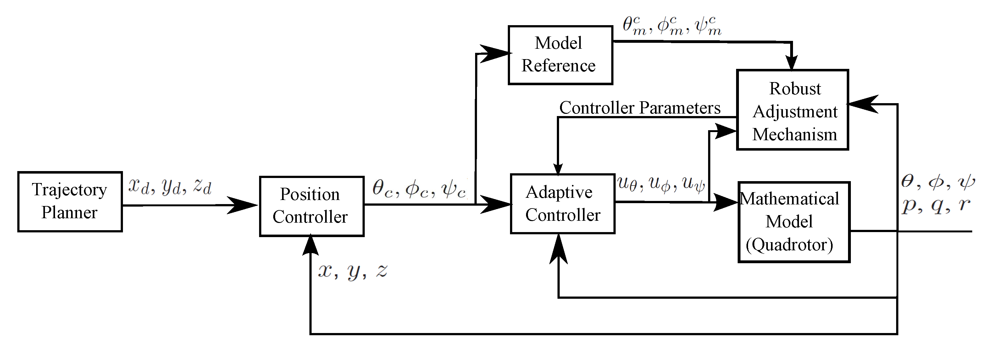
where the gains are ${\alpha }_{p\Theta },{\alpha }_{v\Theta }>0$. Thus, with the MIT-HOSM, a robust adjustment mechanism is obtained and is reduced or almost eliminates the undesired chattering effect. In Figure 3, the block diagram of the adaptive robust system is shown.

Trajectory Following

The control objective is for the quadrotor to follow a predefined trajectory generated by a trajectory planner to develop an adequate flight plan for the quadrotor. In Section 3, the trajectory to follow and the trajectory planner are described mathematically. The angles with more dynamics to follow the desired trajectory are the pitch and roll angles, these angles change between $\pm {10}^{\circ }$, and the yaw angle is $5^{\circ }$ during the trajectory. 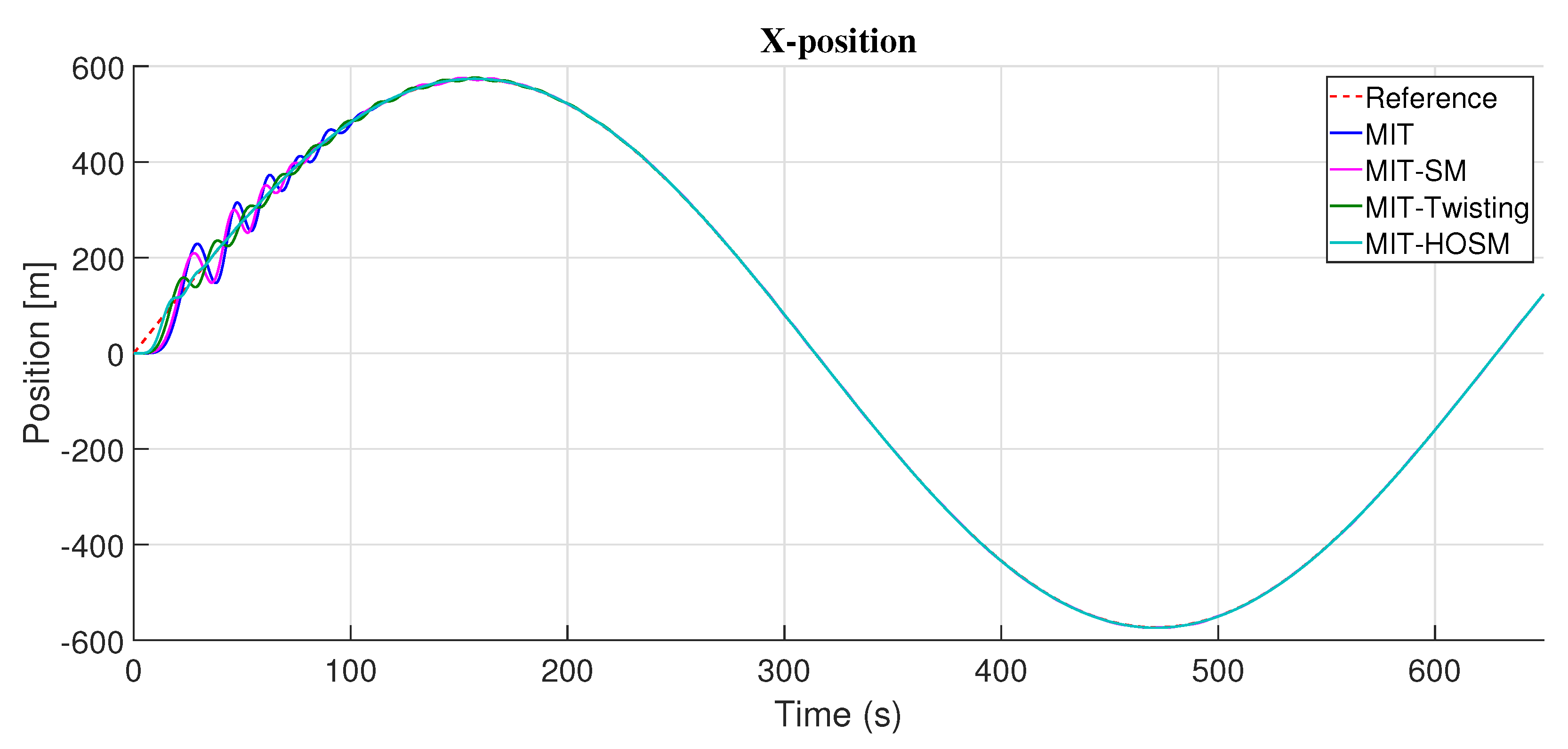Figure 4 presents the response of the adaptive controller with the different adjustment mechanisms proposed in this work; significant oscillations over the desired position are appreciated in axis-x by the adaptive controller based on the MIT, MIT with sliding modes (MIT-SM), and MIT with twisting (MIT-Twisting). The adjustment mechanism MIT with high order sliding mode (MIT-HOSM) presented smaller oscillations, and the convergence time to the desired reference is less than the adjustment mechanism MIT, MIT-SM, and MIT-Twisting; see Figure 4.

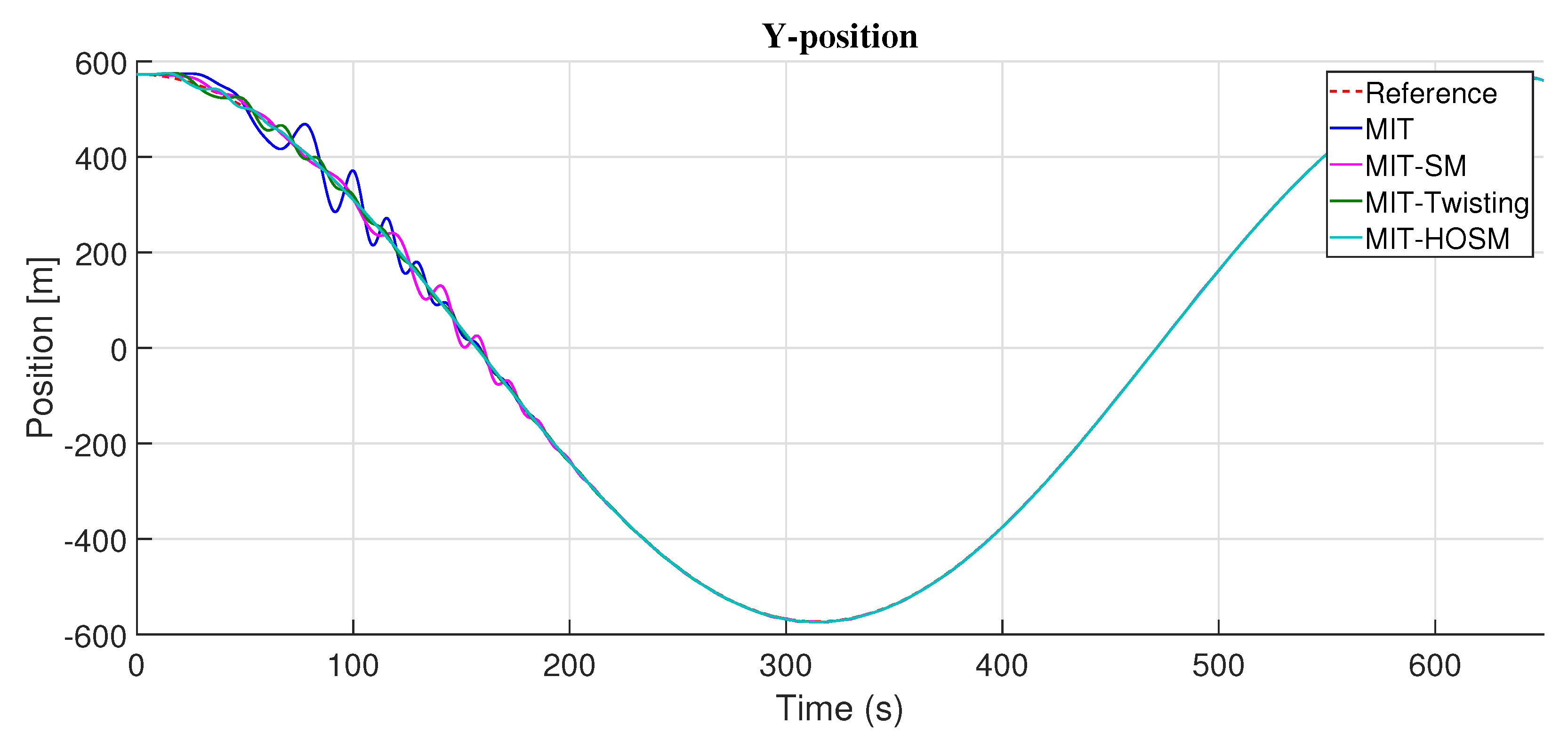
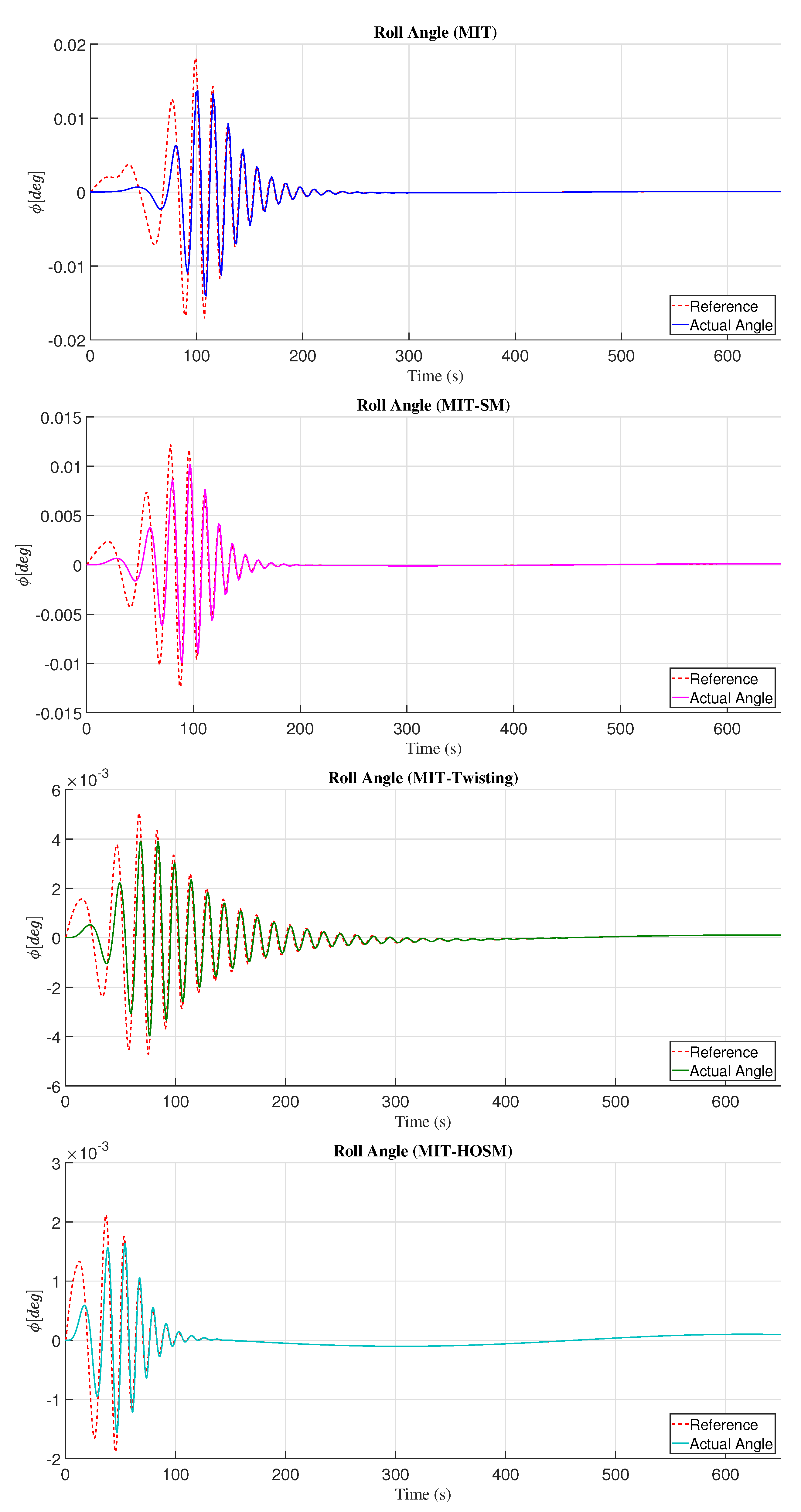
Figure 5 presents the results obtained with the PD adaptive controller and the adjustment mechanism based on the MIT and sliding mode techniques. Oscillations are appreciated before converging to the desired reference with the adjustment mechanism based on MIT, MIT with sliding mode (MIT-SM), and MIT with twisting (MIT-Twisting). On the other hand, the adjustment mechanism MIT with high order sliding mode presented a better response with minor oscillations and convergence to the desired position in less time over the y axis. 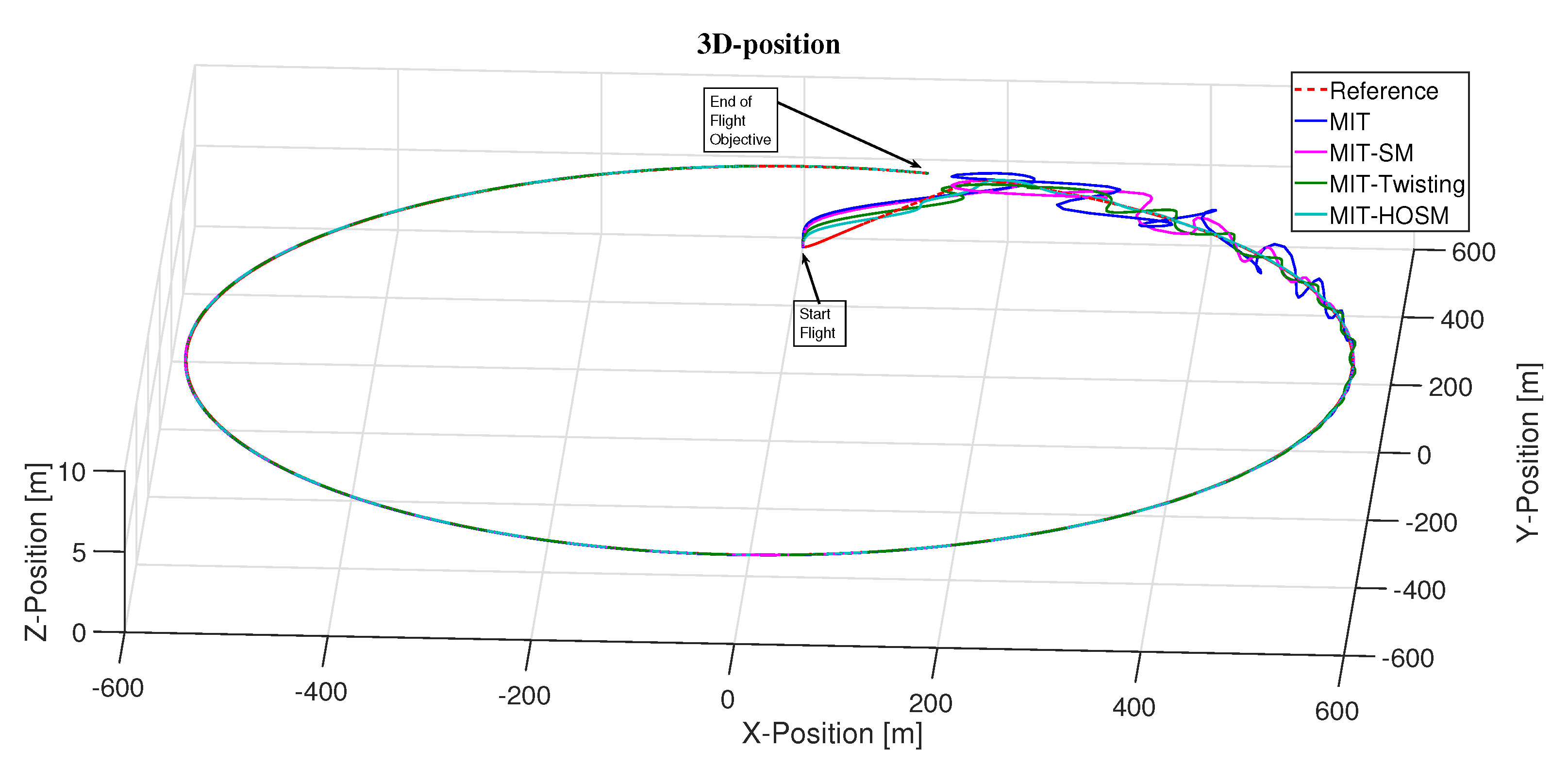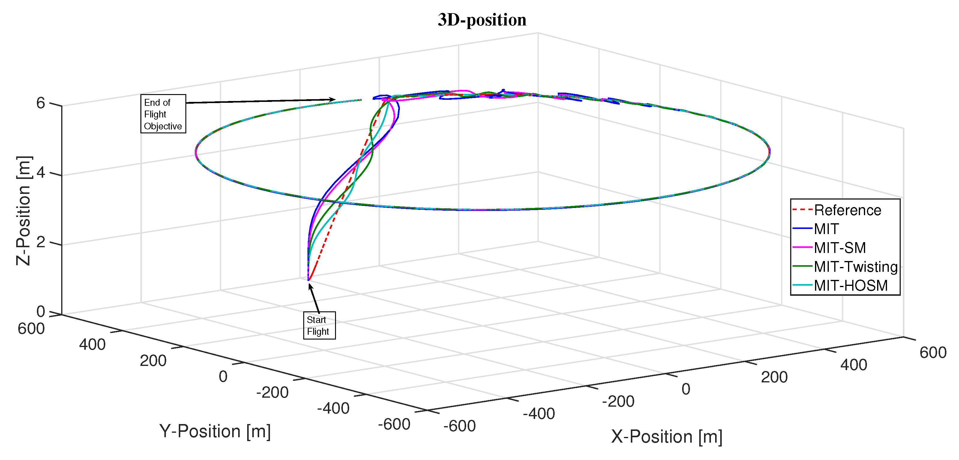In Figure 6, a top perspective or top 3D view is presented to appreciate the oscillations mentioned before the desired trajectory (reference) that is followed by the quadrotor; in this figure, the PD adaptive control with the four different adjustment mechanisms proposed in this work is represented. Figure 7 presents a 3D image that represents the flight of the quadrotor with the PD adaptive controller with the different adjustment mechanisms proposed in this work.

In this work, the ${\mathcal{L}}_2$-norm [33] is used to know the error and control signal response in a numerical form. Thus, the definition of the ${\mathcal{L}}_2\left[{\overrightarrow{e}}_{{\Theta }_m^c}\right]$ correspond to analyze error signals and the ${\mathcal{L}}_2\left[u_{\Theta }\right]$ correspond to controller output signals:

$${\mathcal{L}}_2\left[{\overrightarrow{e}}_{{\Theta }_m^c}\right]=\sqrt{\frac{1}{T-t_0}{\int }_{t_0}^T{\parallel {\overrightarrow{e}}_{{\Theta }_m^c}|}^{2}dt}$$

(30)

$${\mathcal{L}}_2\left[u_{\Theta }\right]=\sqrt{\frac{1}{T-t_0}{\int }_{t_0}^T{\parallel u_{\Theta }\parallel }^{2}dt}$$

(31)

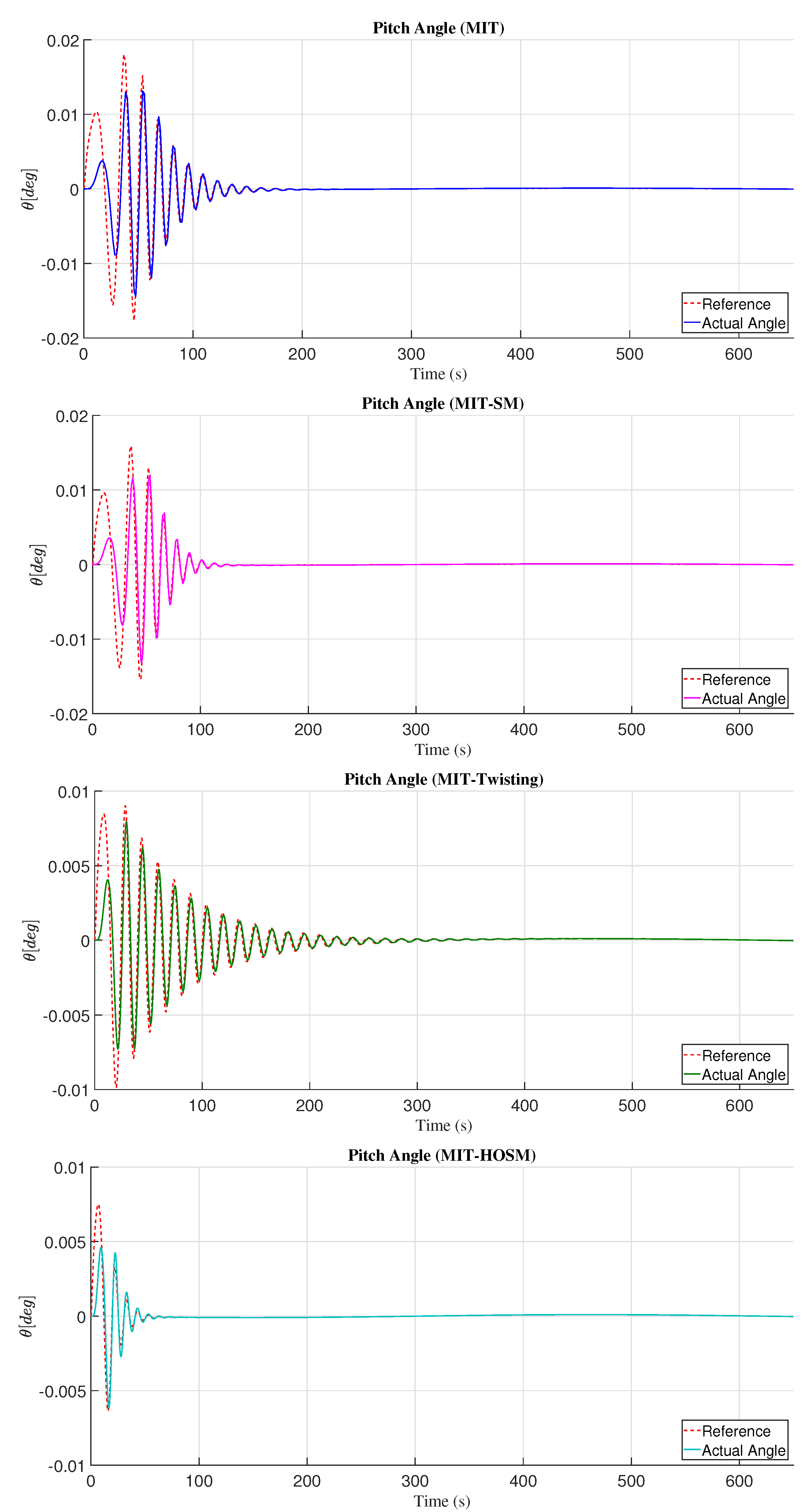
Figure 8 presents the results obtained with the PD adaptive controller with the adjustment mechanism based on the methodology MIT rule and the theory by sliding modes (MIT-SM), twisting (MIT-Twisting), and high order sliding mode (MIT-HOSM). Considering the analysis with the ${\mathcal{L}}_2\left[{\overrightarrow{e}}_{{\Theta }_m^c}\right]$ to know the error presented in the pitch angle, the adjustment mechanism with MIT rule the error in pitch angle is bigger than MIT with sliding mode (MIT-SM), MIT with twisting (MIT-Twisting), and MIT with high order sliding modes (MIT-HOSM). Then, the adaptive controller based on the MIT with high order sliding mode (MIT-HOSM) presented a more minor error than MIT, MIT-SM, and MIT-Twisting (see

Table 1. Numerical results with ${\mathcal{L}}_2$ of the adaptive robust controllers in pitch angle.

Controller	Pitch [deg]
	${\mathcal{L}}_2\left[e_{{\theta }_c}\right]$	${\mathcal{L}}_2\left[u_{\theta }\right]$
MIT	0.5452	0.1565
MIT-SM	0.5333	0.1528
MIT-Twisting	0.0051	0.0170
MIT-HOSM	0.0026	0.0097

).

On the other hand, for pitch angle, the PD adaptive controller, which applied a bigger control response to achieve the control objective, is the adjustment mechanism based on the MIT rule. The controller that applied smaller effort to achieve the control objective is MIT’s adjustment mechanism with high order sliding mode. This is verified by the analysis results obtained with ${\mathcal{L}}_2\left[u_{\Theta }\right]$ in Table 1.

On the other hand, for pitch angle, the PD adaptive controller, which applied a bigger control response to achieve the control objective, is the adjustment mechanism based on the MIT rule. The smaller effort to achieve the control objective is MIT’s adjustment mechanism with high order sliding mode. It is verified by the analysis results obtained with ${\mathcal{L}}_2\left[u_{\Theta }\right]$ in Table 1.

Thus, the adjustment mechanism based on the MIT rule of the control effort ${\mathcal{L}}_2\left[u_{\Theta }\right]$ to achieve the control objective is bigger than the MIT-SM, MIT-Twisting, and MIT-HOSM. On the other hand, the adjustment mechanism based on the MIT-HOSM presented a smaller effort to achieve the desired roll angle than the based on MIT, MIT-SM, and MIT-Twisting. The results obtained are present in

Table 2. Numerical results with ${\mathcal{L}}_2$ of the adaptive robust controllers in roll angle.

Controller	Roll [deg]
	${\mathcal{L}}_2\left[e_{{\varphi }_c}\right]$	${\mathcal{L}}_2\left[u_{\varphi }\right]$
MIT	0.5191	1.15806
MIT-SM	0.3571	1.12103
MIT-Twisting	0.0029	0.0094
MIT-HOSM	0.0011	0.0033

, and in Figure 9 the response of the roll angle is presented with the PD adaptive controller with the different adjustment mechanism proposed in this work.

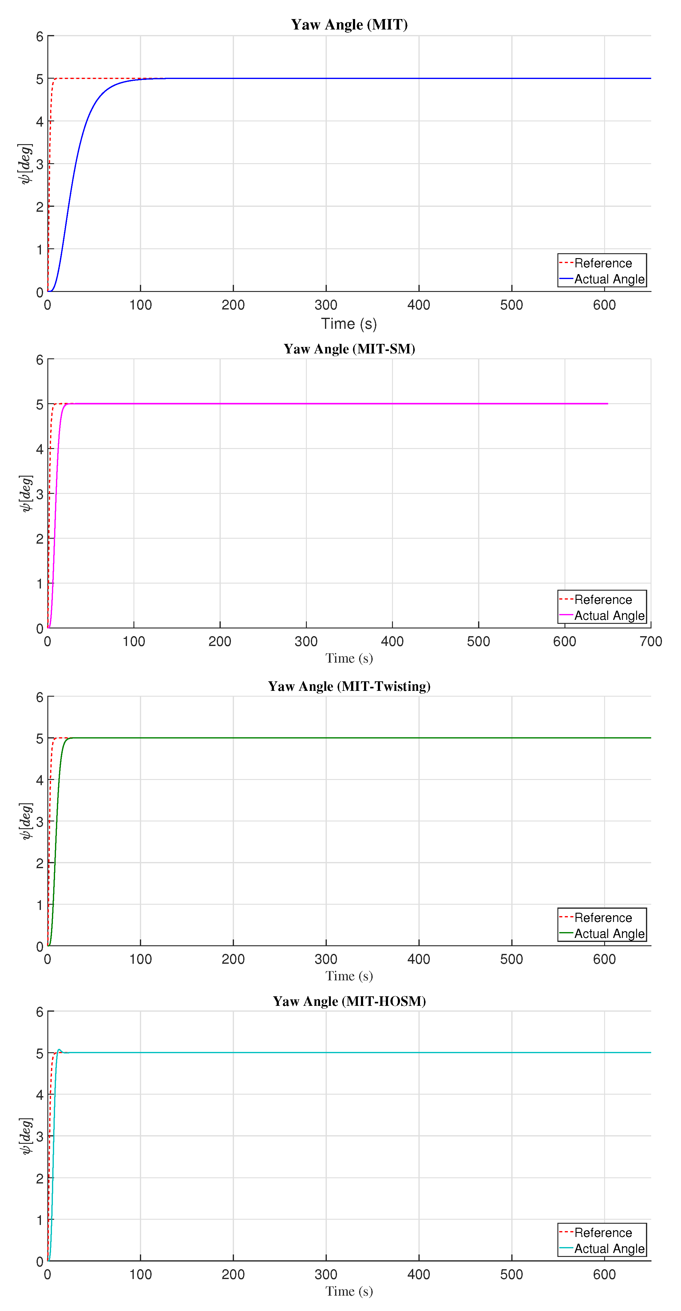
Analyzing the yaw angle with (30) and (31), the PD adaptive controller which presented a smaller error is the adjustment mechanism based on the MIT with sliding modes (MIT-SM) than the MIT, MIT-Twisting, and MIT-HOSM; see

Table 3. Numerical results with ${\mathcal{L}}_2$ of the adaptive robust controllers in yaw angle.

Controller	Yaw [deg]
	${\mathcal{L}}_2\left[e_{{\psi }_c}\right]$	${\mathcal{L}}_2\left[u_{\psi }\right]$
MIT	0.0249	0.0135
MIT-SM	0.0134	0.0292
MIT-Twisting	2.0546	4.8103
MIT-HOSM	1.4752	6.6313

. Furthermore, the adaptive control based on the adjustment mechanism for the yaw angle with a bigger error is the MIT with Twisting (MIT-Twisting). On the other hand, the adaptive controller’s adjustment mechanism, which presented a greater control effort to achieve the control objective, is based on the MIT with high order sliding mode (MIT-HOSM). The MIT rule showed a smaller control effort than the MIT-SM, MIT-Twisting, and MIT-HOSM. In Figure 10 the response of the yaw angle is presented with the PD adaptive controller with the different adjustment mechanism proposed in this work.

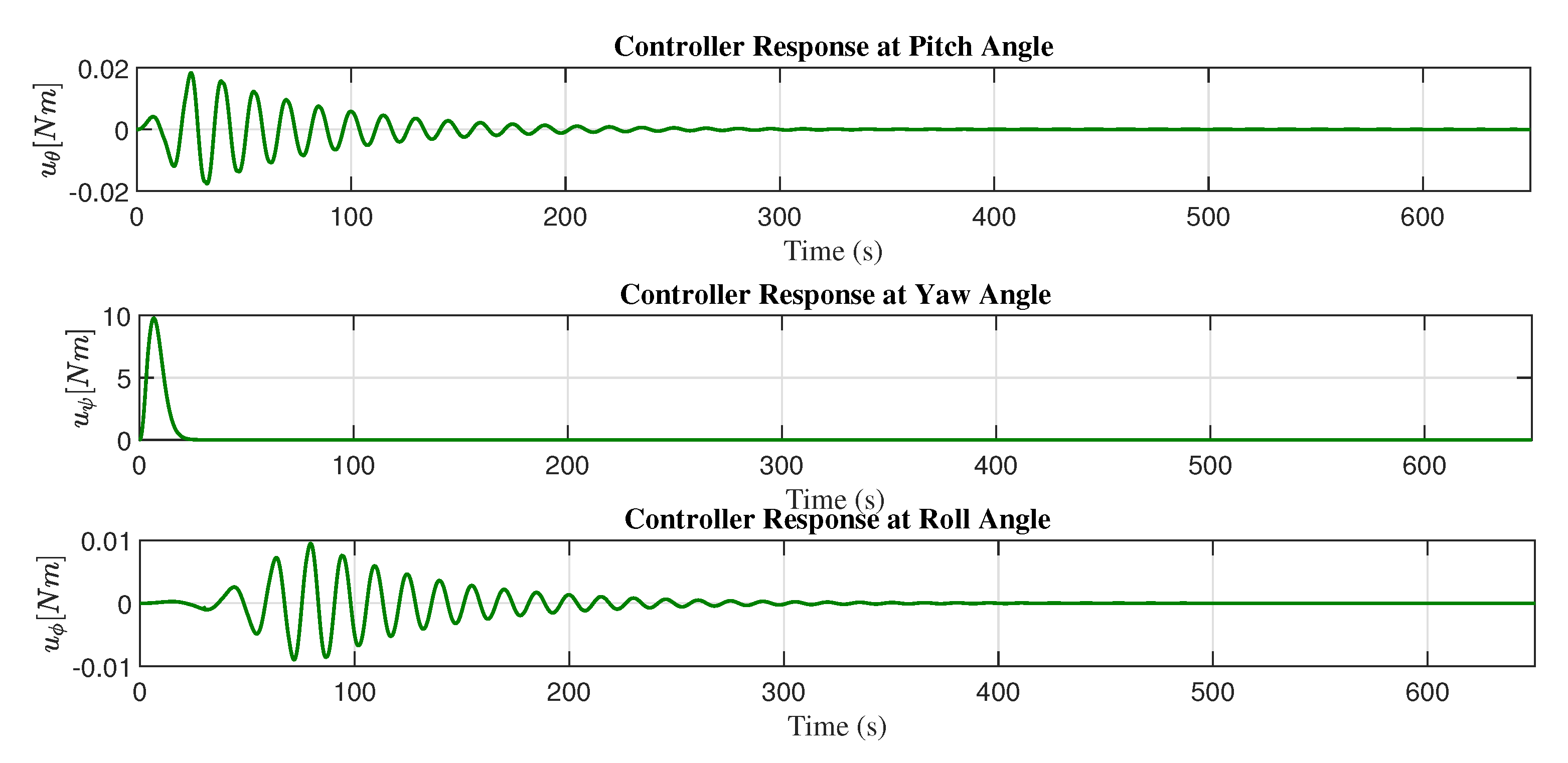
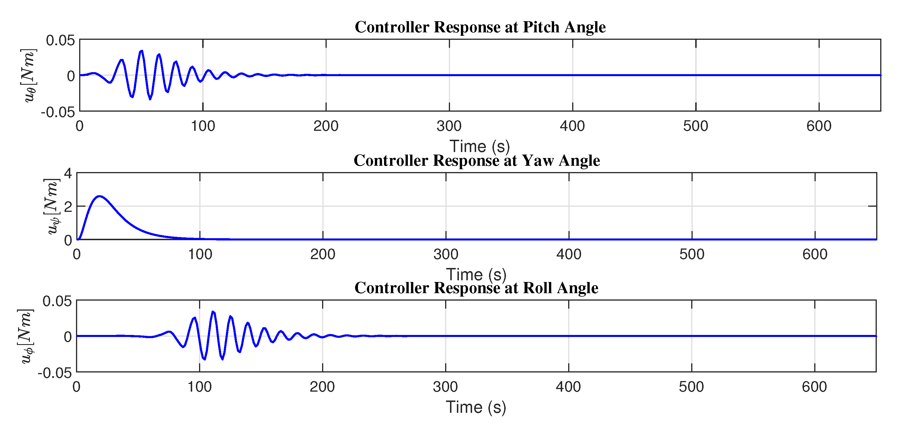
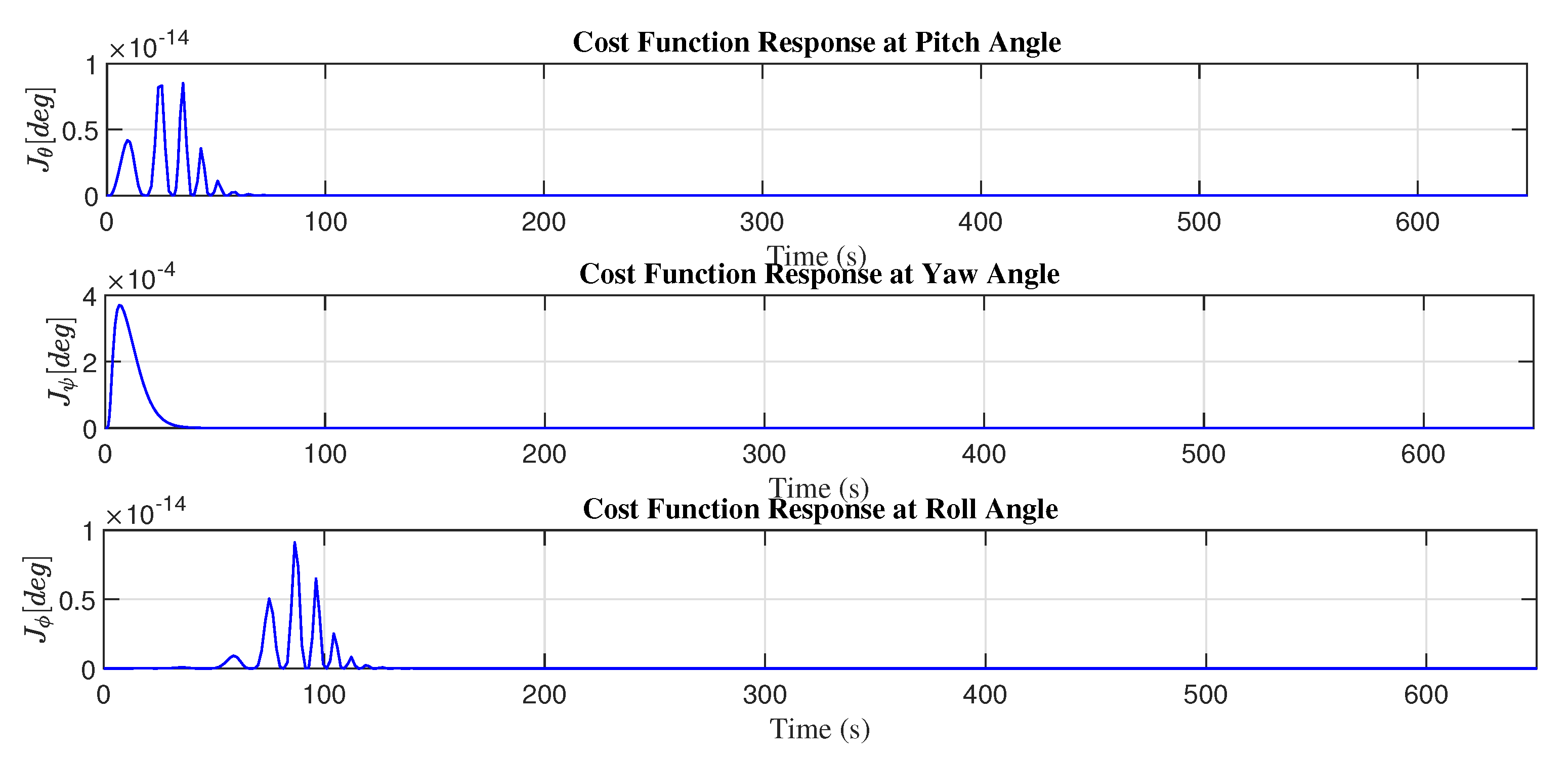
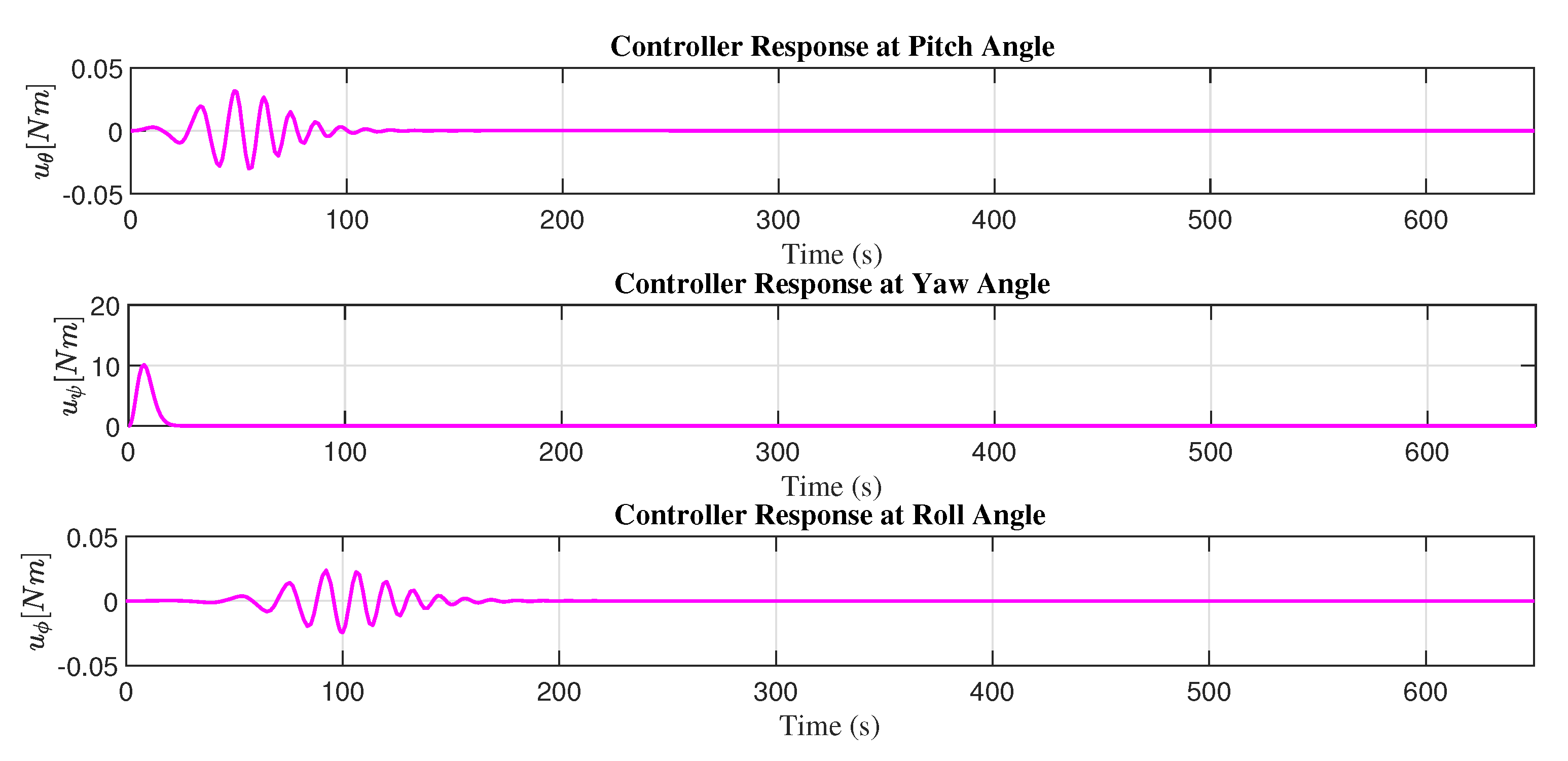
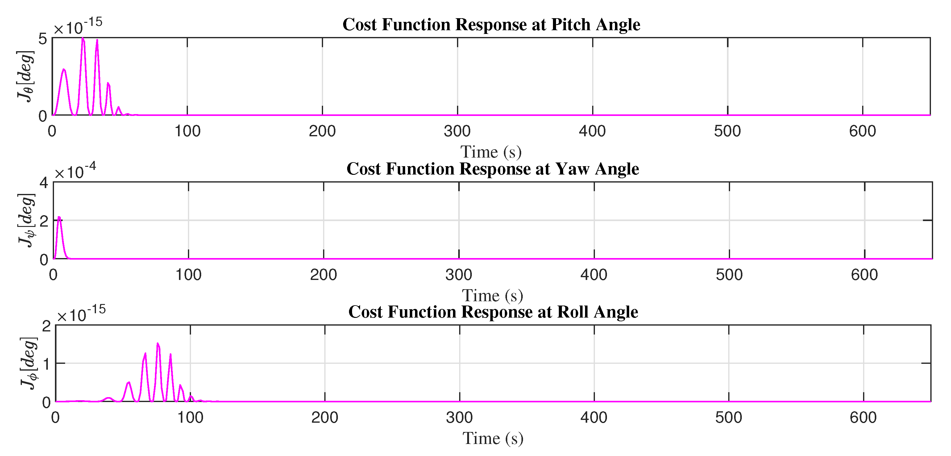
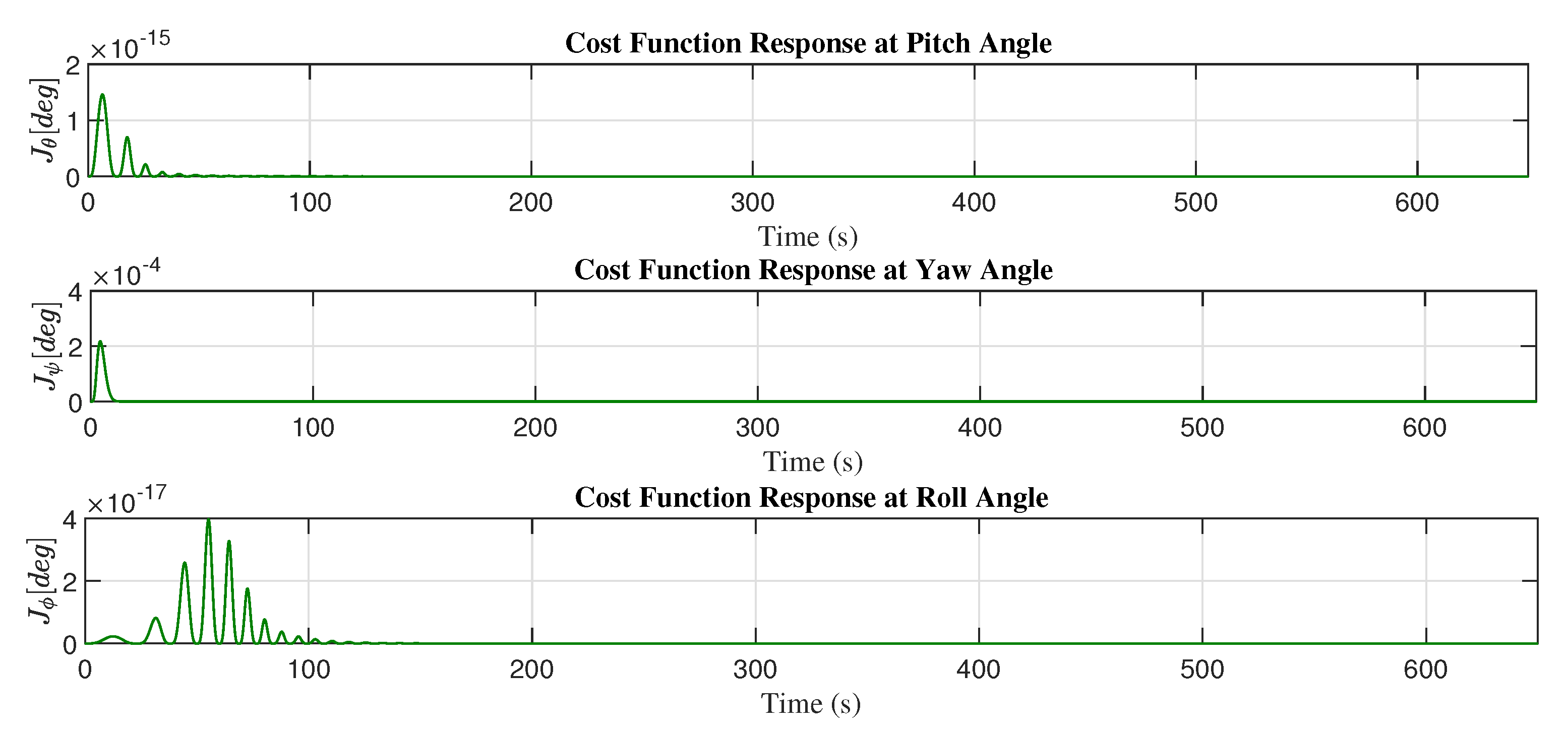
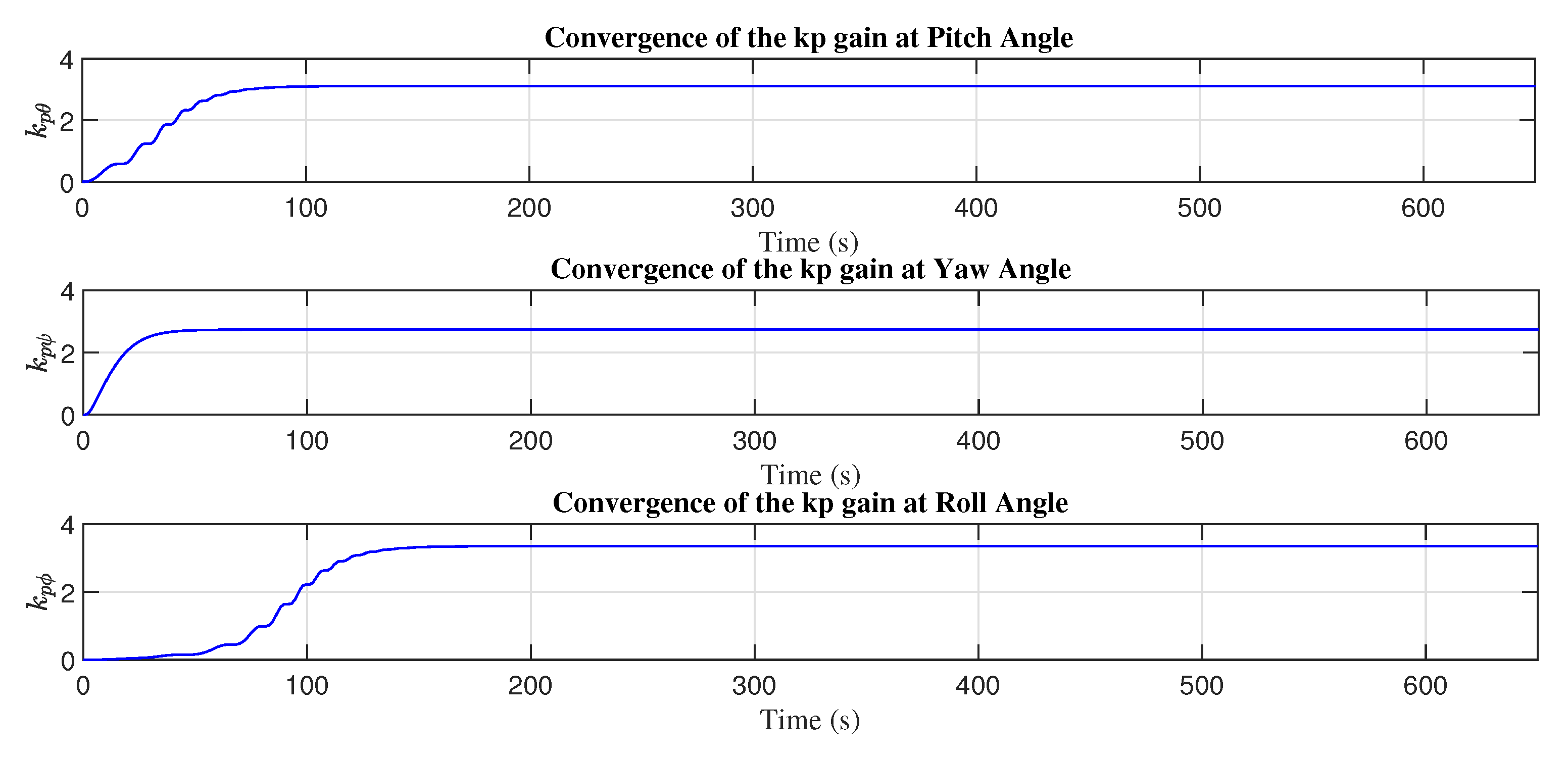
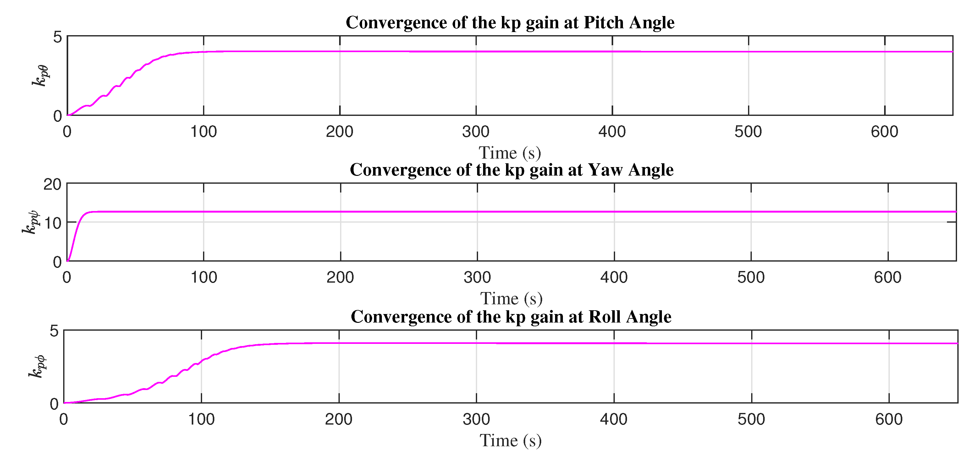
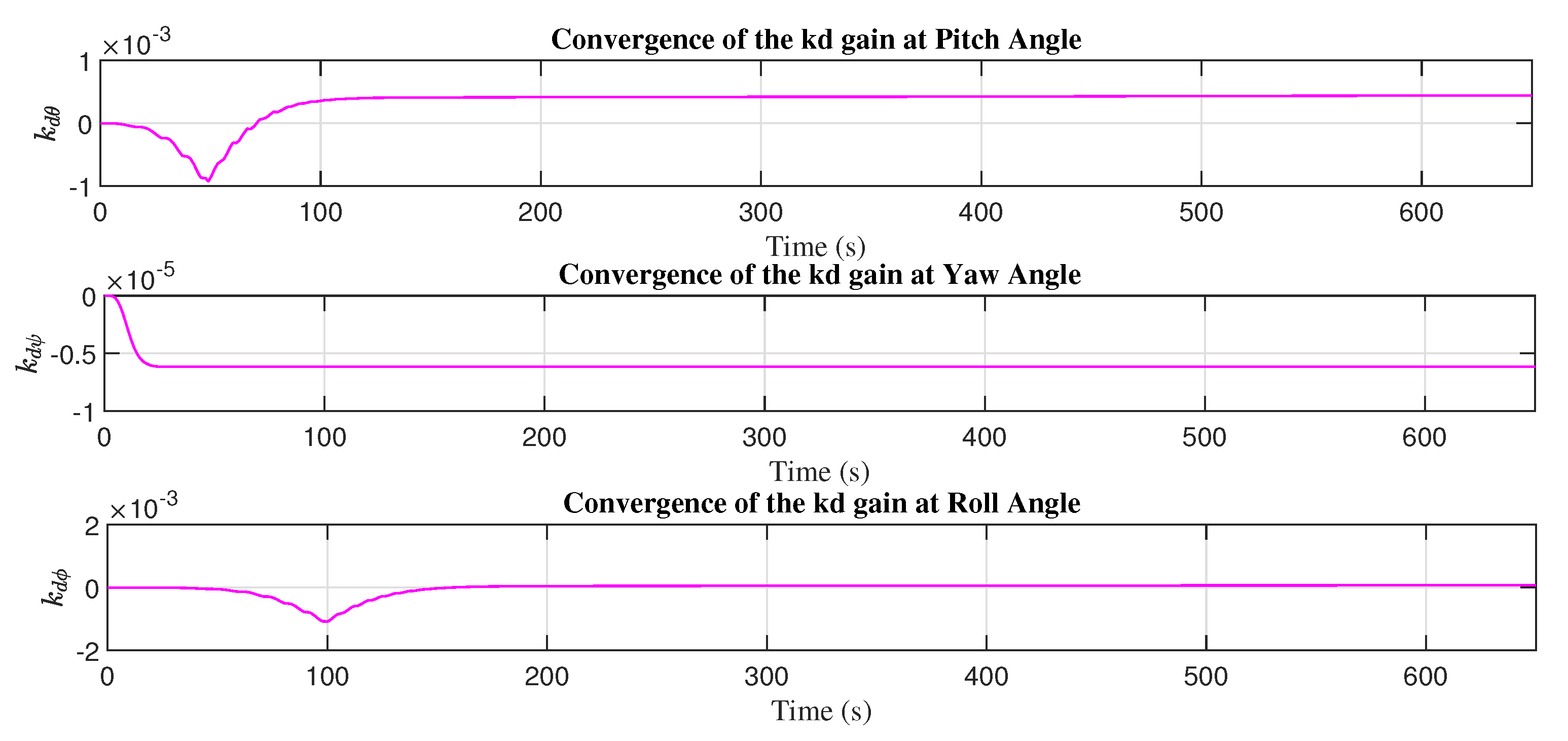
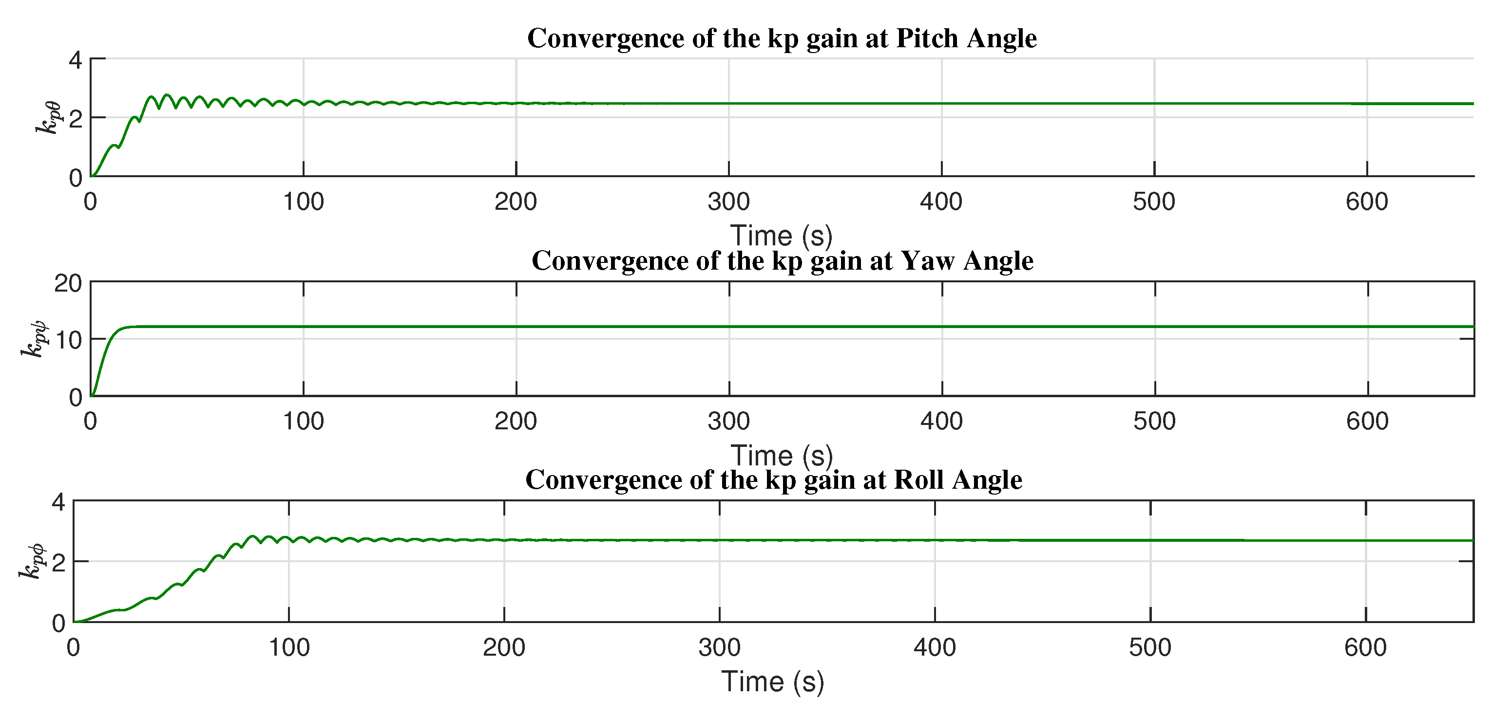
In Figure 11, the control response of the PD adaptive controller is presented with the adjustment mechanism based on the MIT rule, and Figure 12 shows the minimization of the cost function with the adaptive control law and the adjustment mechanism based on the MIT rule. Figure 13 and Figure 14 present the convergence of the adaptive gains with the adjustment mechanism based on the MIT rule.

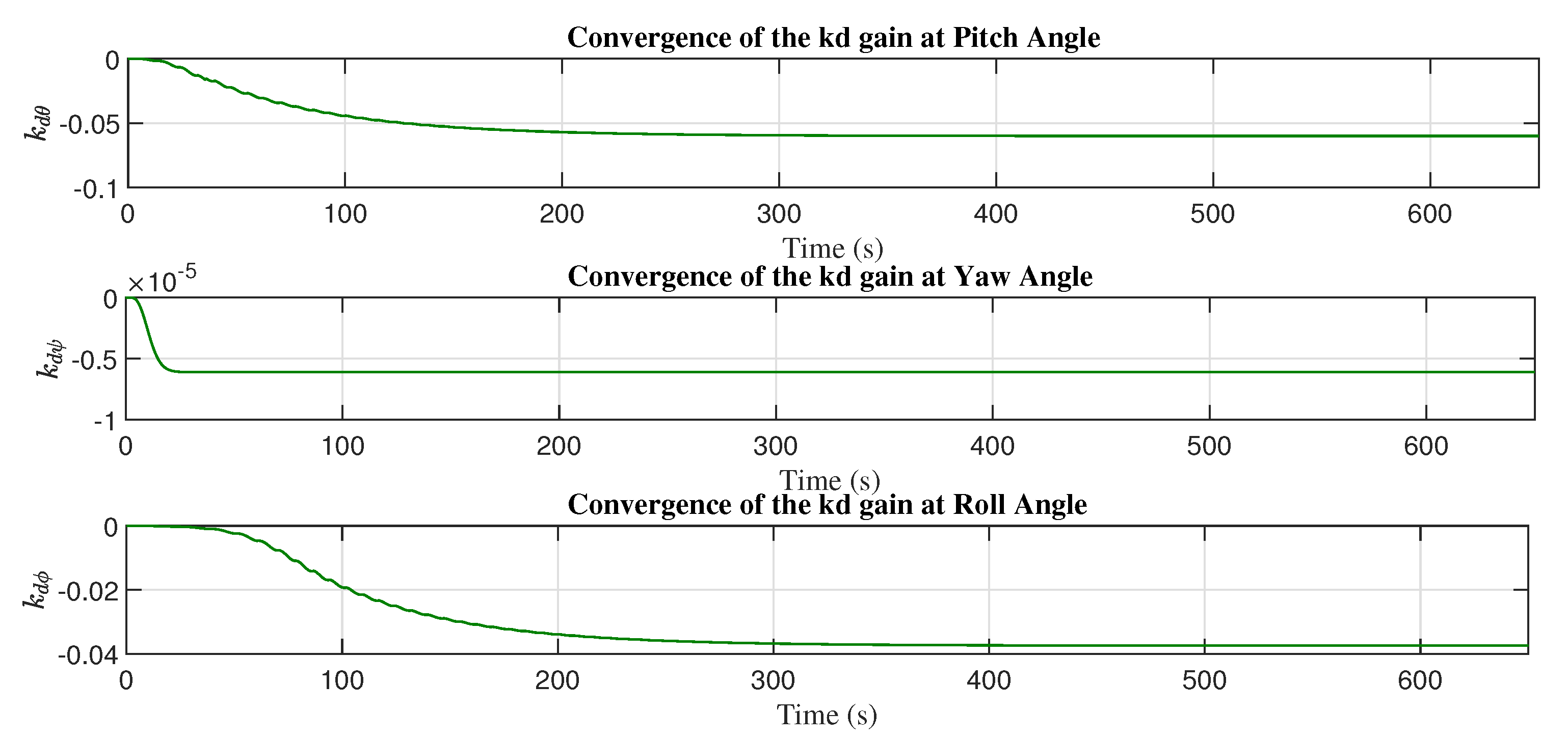
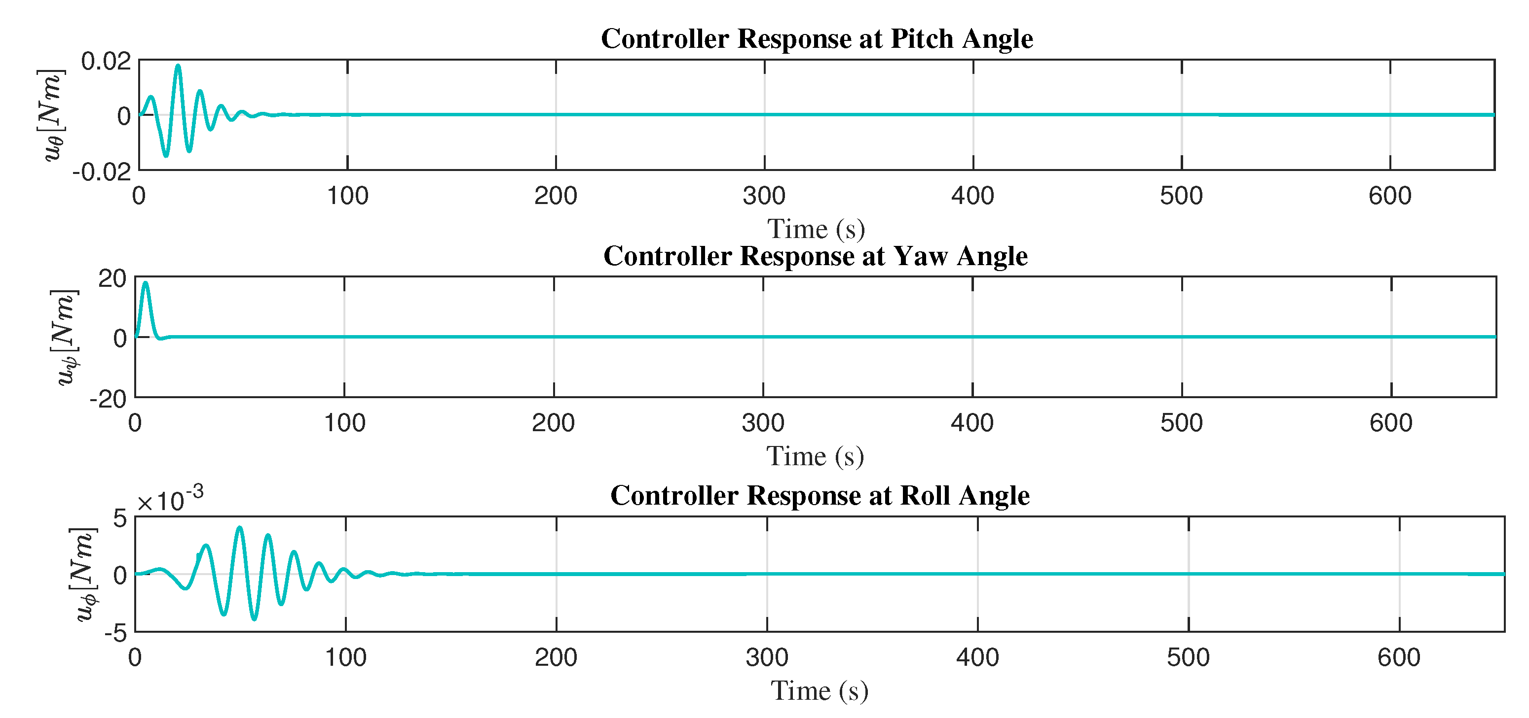
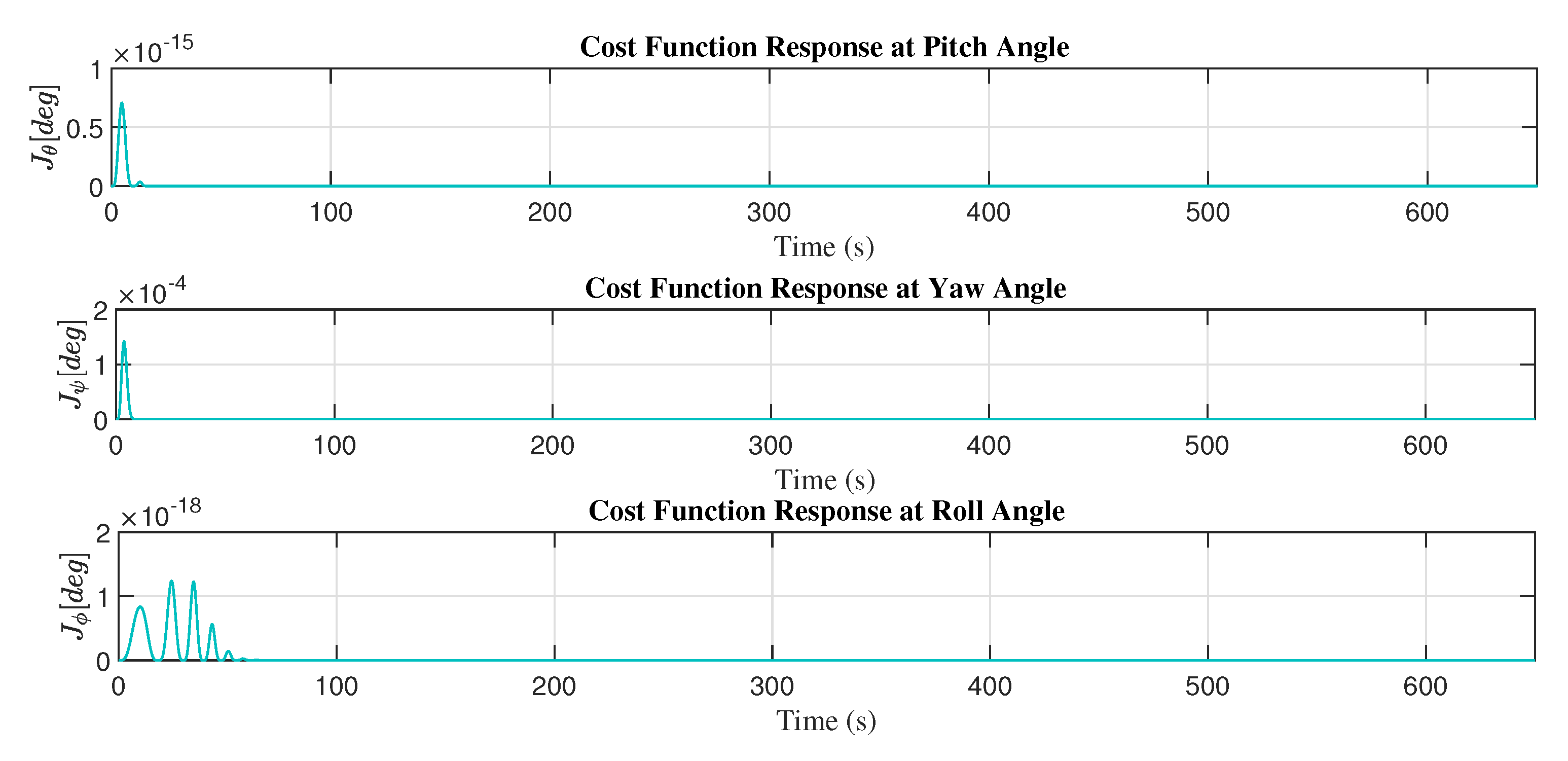
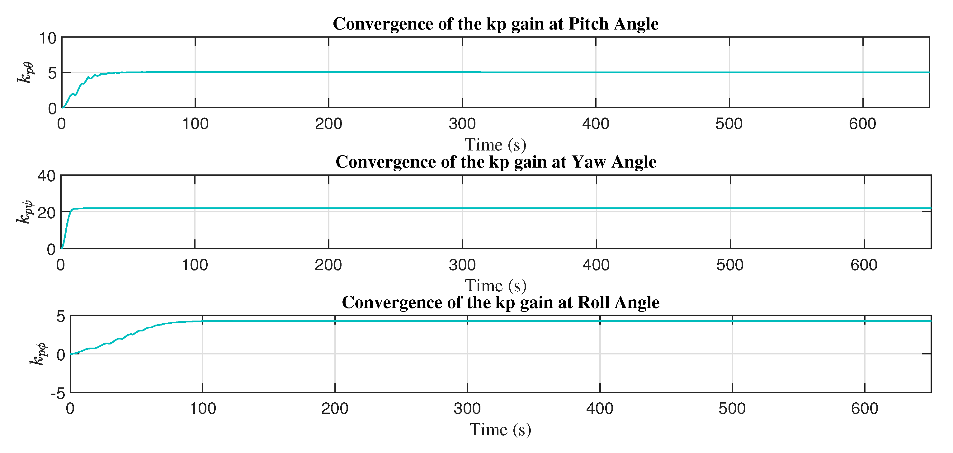
Figure 15 shows the control response of the adaptive controller based on the MIT rule with sliding mode (MIT-SM). Figure 16 presents the minimization of the cost function with MIT-SM, and Figure 17 and Figure 18 presents the convergence of the adaptive gains with the adaptive mechanism based on the MIT rule with sliding mode (MIT-SM).

The control response to achieve the desired trajectory with the adaptive control law with MIT rule with twisting (MIT-Twisting) is presented in Figure 19. The minimization of the cost function with MIT-Twisting illustrates in Figure 20. Figure 21 and Figure 22 present the convergence of the adaptive gains with the adjustment mechanism MIT-Twisting.

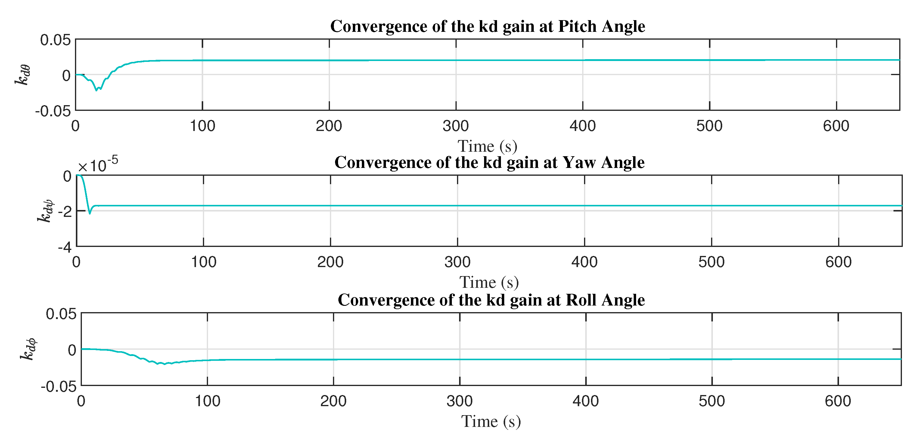
Figure 23 shows the control response with the adaptive control and the adjustment mechanism based on the MIT rule with high order sliding mode (MIT-HOSM). Figure 24 presents the minimization of the cost function with the adaptive controller and MIT-HOSM-like adjustment mechanism. Figure 25 and Figure 26 present the convergence of the adaptive control gains.

5. Discussion

The problem of trajectory tracking with a quadrotor after several simulations is that the PD adaptive controller with the adjustment mechanism based on the MIT rule methodology, and the model reference adaptive control for MRAC, is not enough to resolve the problem due to the oscillations at the beginning of the desired trajectory. This implies that the quadrotor flight is so far from the desired trajectory and the convergence time is too slow (see Figure 6 and Figure 7); for that reason, it is necessary to design a robust adjustment mechanism with a robust theory like that based on sliding modes.

Then, the adjustment mechanism MIT rule with sliding mode (MIT-SM) reduced the oscillations in the trajectory tracking with the quadrotor and a better convergence time. Besides, the MIT rule with the twisting (MIT-Twisting) adjustment mechanism presents a better response in convergence time and oscillation reduction. To obtain the best response in this work to reduce the oscillations (almost eliminate), a short convergence time to the desired trajectory was obtained with the adjustment mechanism based on the MIT rule with high order sliding modes (MIT-HOSM) (see Figure 6 and Figure 7).

Even analyzing the pitch and roll angles, the MIT rule with high order sliding modes (MIT-HOSM) has better error correction. An exception occurs in the yaw angle where the MIT rule with sliding mode (MIT-SM) has a better response in error. On the other hand, we took into account the control effort response with the four proposed adjustment mechanisms. The MIT rule with high order sliding mode (MIT-HOSM) presents the smallest control effort compared to the adjustment mechanisms MIT rule, MIT-Twisting and MIT-HOSM proposed for the pitch and roll angle, except for the yaw angle where the MIT-HOSM applies the biggest control effort to steer the quadrotor for the desired trajectory (see Table 1, Table 2 and Table 3).

Thus, for future work, we have to develop a construction and electronic embedded system for a quadrotor to do real flight tests with the PD adaptive control law with the different robust adjustment mechanisms proposed in this work.